December 2011

Kaluza-Klein Masses and Couplings:
Radiative Corrections to Tree-Level Relations
Sky Bauman^1,2  and  Keith R. Dienes^3,4,2
1 Department of Physics, University of Wisconsin, Madison, WI 53706 USA
² Department of Physics, University of Arizona, Tucson, AZ 85721 USA
³ Physics Division, National Science Foundation, Arlington, VA 22230 USA
⁴ Department of Physics, University of Maryland, College Park, MD 20742 USA

The most direct experimental signature of a compactified extra dimension is the appearance of towers of Kaluza-Klein particles obeying specific mass and coupling relations. However, such masses and couplings are subject to radiative corrections. In this paper, using techniques developed in previous work, we investigate the extent to which such radiative corrections deform the expected tree-level relations between Kaluza-Klein masses and couplings. As toy models for our analysis, we investigate a flat five-dimensional scalar $\lambda\phi^{4}$ model and a flat five-dimensional Yukawa model involving both scalars and fermions. In each case, we identify the conditions under which the tree-level relations are stable to one-loop order, and the situations in which radiative corrections modify the algebraic forms of these relations. Such corrections to Kaluza-Klein spectra therefore have the potential to distort the apparent geometry of a large extra dimension.

1 Introduction

The existence of Kaluza-Klein (KK) states is perhaps the most important phenomenological prediction of extra dimensions, and any future search for physics beyond the Standard Model will involve a hunt for signs of these particles. For this reason, it is vital to understand the properties of these states and the effects that they induce on low-energy physics. Of course, one important way in which excited KK states can affect low-energy physics is through the radiative corrections that they induce for zero-mode masses and couplings. Indeed, over the past decade, a significant body of literature has developed in which this topic is studied in a variety of contexts and from a variety of perspectives.

However, with only a few exceptions, relatively little attention has been paid to the radiative effects that the excited KK states may have on their own masses and couplings. Since these excited KK states are likely to be our only direct experimental probes into the apparent geometry of the compactification manifold, it is important to understand the extent to which such radiative corrections can distort the expected tree-level relations that the KK masses and couplings can be expected to satisfy, and which would ultimately be used as evidence of a geometric underpinning for such states.

To help sharpen the discussion, let us consider the simplest possible case of a single extra dimension compactified on a circle. At tree level, the masses of the corresponding KK states can be expected to obey the well-known dispersion relation

$$m_{n}^{2}~{}=~{}m^{2}+\frac{n^{2}}{R^{2}}~{}$$ (1.1)

where $m_{n}$ is the mass of the $n^{\rm th}$ KK mode, where $m$ is the “bare” mass associated with our original five-dimensional field, and where $R$ is the radius of the extra dimension. Note that this result assumes only that the extra dimension is flat and that the original theory obeys five-dimensional (5D) Lorentz symmetry. Likewise, at tree level, the couplings in a Lorentz-invariant theory on an extra dimension are universal, independent of mode number. Specifically, if $\lambda_{n,n^{\prime},...}$ represents a tree-level coupling between KK modes $(n,n^{\prime},...)$, then

$$\lambda_{n,n^{\prime},...}~{}=~{}\lambda\,\delta_{n+n^{\prime}+...,0}~{}$$ (1.2)

where $\lambda$ is a constant related to the five-dimensional “bare” coupling and where the delta-function enforces 5D momentum conservation at the associated vertex. The important point is that $\lambda_{n,n^{\prime},...}$ takes this highly restricted form, depending on the KK mode numbers $(n,n^{\prime},n^{\prime\prime},...)$ only insofar as they determine whether the coupling vanishes or takes a fixed, mode-independent value.

Like the masses and couplings in any theory, however, the masses and couplings of KK states can receive radiative corrections. Thus, it is possible that the tree-level relations in Eqs. (1.1) and (1.2) will no longer hold once these masses and couplings are replaced by their one-loop renormalized values. At first glance, it might seem that the forms of Eqs. (1.1) and (1.2) are fixed by 5D Lorentz invariance. However, we must recall that 5D Lorentz invariance is actually broken by the compactification from five to four dimensions. The effects of this compactification are what allow more complicated dispersion relations to emerge in the fully quantum-mechanical theory.

Focusing specifically on the mass relation in Eq. (1.1), we can imagine a number of potential outcomes depending on the specific theory in question. One possibility is that the one-loop renormalized KK masses will continue to obey a relation that preserves the form of Eq. (1.1) — i.e., that all radiative corrections can be bundled into a new effective bare mass $m$ or a new effective radius $R$. Despite the fact that $m$ and $R$ are merely fixed parameters describing our ultraviolet theory, we shall refer to these outcomes as effective “renormalizations” of these quantities. However, the breaking of 5D Lorentz invariance might also allow the spectrum of renormalized KK masses to have an entirely new dependence on mode number, implying that even the forms of the tree-level relations might be violated.

More precisely, we can classify the different types of quantum corrections that our squared KK masses may experience:

• Case #1: The corrections to each $m_{n}^{2}$ are independent of mode number $n$. In this case, the bare mass $m$ is effectively renormalized, but the KK dispersion relation retains the same mathematical form as it had at tree level. In this case, 5D Lorentz invariance is preserved locally. However, since compactification breaks 5D Lorentz invariance globally by singling out the compactified extra dimension, this occurrence would be entirely unexpected. We shall nevertheless give an example where this phenomenon arises to one-loop order in Sect. 3.

• Case #2: The corrections to $m_{n}^{2}$ are proportional to the square of the mode number $n$. In this case, we can bundle the renormalizations into an effective rescaling or renormalization of the radius $R$. To the extent that the radius is an arbitrary parameter and the form of the general KK mass relation is preserved, this also would not indicate a direct local breaking of 5D Lorentz invariance. As such, this case would also be unexpected, just like Case #1 above. However, since such radiative corrections would manifest themselves as effectively modifying the value of $R$, it would appear that our underlying compactification geometry is distorted somewhat, with the radius of the circle shifting slightly. We stress, however, that this is not an actual geometric effect since the underlying compactification geometry is presumably unchanged (unless there are also renormalizations of the higher-dimensional metric). This is therefore merely a change in the apparent compactification geometry, as inferred through the masses of KK states.

• Case #3: The corrections to $m_{n}^{2}$ depend on mode number $n$ non-quadratically. In this case, it turns out that there is a particularly relevant division into two sub-cases which we shall consider:

  • Case #3a: The masses of an infinite subset of states in the KK tower shift according to Case #1 or Case #2 (corresponding to shifts in the values of $m$ or $R$), but this is not true of the entire KK tower. Thus, the KK dispersion relation is broken for the KK tower on a whole. We shall refer to this as an implicit violation of the KK dispersion relation.

  • Case #3b: The KK dispersion relation does not survive for any infinite subset of states in the KK tower. We shall refer to this as an explicit violation of the KK dispersion relation.

  In this paper, we shall see explicit examples of both of these cases. Note that for either of these two sub-cases, the KK masses as a whole no longer obey Eq. (1.1). It would therefore seem that these KK states could no longer be identified as the Kaluza-Klein excitations of a quantum field compactified on a circle — i.e., the apparent compactification geometry of the extra dimension would appear distorted in such a way in such cases that not even an underlying circle is recognizable.

In this paper, our goal is to begin to develop an understanding of the sorts of theories which might lead to corrections in each class. Towards this end, we shall therefore study two “toy” models: $\phi^{4}$ theory and Yukawa theory, each in five dimensions with a single extra dimension compactified on a circle. For each of these two theories, we shall obtain results for the radiative corrections to the masses and couplings of the KK modes, and examine the properties of the physics which results.

Both of these toy models may ultimately be relevant to the Higgs sector of the 5D Standard Model. Despite this fact, we emphasize that the primary purpose of this paper is not phenomenological, and indeed many of these radiative corrections will turn out to be numerically fairly small. Rather, our primary focus will be on the mathematical forms of the radiative corrections that emerge in each case, and on the general mathematical patterns that describe the deformations of KK masses and couplings which emerge as a result of radiative corrections. For example, one unexpected result we shall find is that the masses of the fermions in the Yukawa theory receive corrections that actually grow with mode number. Another is that a $\gamma^{5}$ interaction is radiatively induced in this theory. Even the $\phi^{4}$ theory will hold some surprises. For example, as we shall demonstrate, radiative corrections tend to enhance the couplings involving the production of excited KK modes.

This paper is organized as follows. First, in Sect. 2, we begin with some general comments concerning renormalization and regulators in “mixed” spacetimes in which some dimensions are compactified and others are not. We also describe the general setup we shall be employing. Then, in Sect. 3, we analyze the $\lambda\phi^{4}$ theory, concentrating on corrections to the masses and couplings of the KK states. In Sect. 4, we then proceed to consider the Yukawa theory; as we shall see, the Yukawa theory is significantly more complex than the $\lambda\phi^{4}$ theory due to the involvement of fermions and issues of parity and chirality. Finally, in Sect. 5, we present our conclusions and discuss how our results connect with other calculations which have previously appeared in the literature.

2 General setup

As stated in the Introduction, our goal is to determine how the tree-level masses and couplings of KK modes behave under renormalization. Before proceeding to examine the cases of specific toy models, however, there are some general remarks which are in order and which will apply to all cases we shall consider.

In general, KK masses and couplings will accrue radiative corrections which are divergent. However, although each of these corrections is individually divergent, the difference between a correction corresponding to an excited KK mode and that corresponding to the zero mode is observable and therefore finite [1, 2]. For example, although the mass of the zero mode and mass of the first excited mode of a KK tower will each generally accrue radiative corrections which are infinite, the difference between these masses (i.e., the mass splitting between these KK modes) is expected to remain finite even after renormalization. The first step in determining such radiative corrections is therefore to recast equations such as Eq. (1.1) into forms whose corrections will be nothing other than these finite differences. In other words, we wish to express these tree-level equations as relations directly between measurable, four-dimensional quantities, eliminating the bare Lagrangian parameters $m$ and $\lambda$ in the process.

In the case of Eq. (1.1), this is not hard to do. Since it follows from Eq. (1.1) that $m_{0}=m$ at tree level, we can rewrite Eq. (1.1) in the tree-level form

$$m_{n}^{2}~{}=~{}m_{0}^{2}+{n^{2}\over R^{2}}~{},$$ (2.1)

whereupon it follows that any possible one-loop radiative correction to this result must be finite and take the form

$$m_{n}^{2}~{}=~{}m_{0}^{2}+{n^{2}\over R^{2}}+\frac{X_{n}^{(m^{2})}}{R^{2}}$$ (2.2)

where $X_{n}^{(m^{2})}$ represents the finite mass correction term. Note that we have chosen to explicitly scale out a factor of $R^{2}$ in this correction term so that the quantity $X_{n}^{(m^{2})}$ is dimensionless.

Given this definition for $X_{n}^{(m^{2})}$ as a relative mass correction, we see that Case #1 from the Introduction corresponds to $X_{n}^{(m^{2})}=0$, while Case #2 corresponds to $X_{n}^{(m^{2})}\sim n^{2}$. By contrast, $X_{n}={\rm constant}\not=0$ is actually an example of Case #3a, since this corresponds to a situation in which all of the excited states in our KK tower have a uniform shift relative to the zero mode. Thus, although the infinite tower of excited states by themselves behave according to Case #1, the entire KK tower (including the zero mode) does not.

In a similar way, we may also recast Eq. (1.2) in the form

$$\lambda_{n,n^{\prime},...}~{}=~{}\lambda_{0,0,...}\,\delta_{n+n^{\prime}+...,0}~{},$$ (2.3)

whereupon a corresponding one-loop equation should take the form

$$\lambda_{n,n^{\prime},...}~{}=~{}\left[\lambda_{0,0,...}+X_{n,n^{\prime},...}^{(\lambda)}\right]~{}\delta_{n+n^{\prime}+...,0}~{}.$$ (2.4)

where $X_{n,n^{\prime},...}^{(\lambda)}$ is likewise a finite coupling correction.

The goal of this paper is to calculate these finite corrections $X^{(m^{2})}_{n}$ and $X^{(\lambda)}_{n,n^{\prime},...}$ to one-loop order in two different theories, and to explore the properties of these corrections. Of course, the emergence of such correction terms ultimately reflects the breaking of the higher-dimensional Lorentz invariance that is induced by the compactification of the fifth dimension on a circle. We remark, however, that although compactification of the fifth dimension breaks 5D Lorentz invariance, translational invariance along the fifth dimension (and thus conservation of the corresponding momenta) is still maintained. It is for this reason that our radiatively corrected couplings $\lambda_{n,n^{\prime},...}$ must still be proportional to an overall Kronecker $\delta$-factor, as indicated in Eq. (2.4).

At first glance, given a specific theory, it might seem to be a rather straightforward exercise to evaluate the radiative corrections $X$ in Eqs. (2.2) and (2.4). However, as discussed in Refs. [1, 2], there are numerous subtleties which come into play. The chief complication is that although we expect our calculations to result in finite relative corrections $X$, the correction to each individual KK mass and coupling will itself be infinite, and we must therefore utilize a particular regulator scheme in order to extract meaningful results. However, in so doing, it is critical that we choose a regulator which preserves not only the four-dimensional Lorentz invariance that remains after the compactification, but also the original higher-dimensional Lorentz invariance which existed prior to compactification. This is because a regulator must, by design, be capable of handling ultraviolet (i.e., local short-distance) divergences, and the physics of the ultraviolet limit is governed by such five-dimensional symmetries in which the global process of compactification plays no role. Moreover, in contexts in which our original higher-dimensional Lagrangian contains a gauge symmetry, our regulator should respect this higher-dimensional gauge invariance as well.

This is an important point. Indeed, use of any regulator which fails to respect the approprite five-dimensional UV symmetries such as 5D Lorentz invariance would introduce spurious, unphysical 5D Lorentz-violating contributions into the $X$ corrections, and it would be difficult to disentangle these spurious contributions from the bona-fide physical effects of the 5D Lorentz violation induced by compactification. This would be completely analogous to calculating a one-loop correction to the photon mass in QED with a regulator that breaks gauge invariance: a non-zero result will generically arise, but this would merely be an artifact of the calculational technique and would not reflect the true underlying physics. Our current situation with 5D Lorentz invariance is similar, except that the compactification itself also induces a breaking of 5D Lorentz symmetry. However, our goal is to study the effects of this compactification (as manifested by the appearance of radiative corrections $X$ that deform the forms of the tree-level KK mass and coupling relations) without mixing such effects with the unphysical effects of having chosen an unsuitable regulator.

In Refs. [1, 2], two regulators were developed that can handle precisely such calculations. These are the so-called “extended hard cutoff” (EHC) regulator scheme and the so-called “extended dimensional regularization” (EDR) scheme. Although based on traditional four-dimensional regulators, the key new feature of these higher-dimensional regulators is that they are specifically designed to handle mixed spacetimes in which some dimensions are infinitely large and others are compactified. Moreover, unlike most other regulators which have been used in the extra-dimension literature, these regulators are designed to respect the original higher-dimensional Lorentz symmetries that exist prior to compactification, and not merely the four-dimensional symmetries which remain afterward. As we have discussed above, this distinction is particularly relevant for calculations of the physics of the excited Kaluza-Klein modes themselves, and not merely their radiative effects on zero modes. By respecting the full higher-dimensional symmetries, our regulators avoid the introduction of spurious terms which would not have been easy to disentangle from the physical effects of compactification.

Using the regulators developed in Refs. [1, 2], we can evaluate the corrections $X$ to one-loop order in a variety of different theories. Regardless of the theory, however, it turns out [1, 2] that one-loop radiative corrections $X_{n}$ with a single KK index $n$ can generally be expressed in the form

$$X_{n}~{}=~{}\sum_{r=-\infty}^{\infty}\frac{1}{|n|}\sum_{j=0}^{|n|-1}\int_{0}^{1}dv\left[\alpha_{n}(r,v,j)-\alpha_{0}(r,v)\right]$$ (2.5)

where $\alpha_{0}$ and $\alpha_{n}$ are finite, regulator-independent functions and where the summations and integration in Eq. (2.5) are all absolutely convergent. Here $v$ is a Feynman parameter, and it is assumed that all of the relevant diagrams involved in such radiative corrections can be evaluated with the use of a single Feynman parameter. Indeed, an expression analogous to Eq. (2.5) is available in certain cases requiring multiple Feynman parameters [1], and we shall see an example of this in Sect. 4.

At first glance, the result in Eq. (2.5) might not seem particularly noteworthy. After all, an expression of this general form arises immediately upon a straightforward application of the Feynman rules, with appropriate one-loop integrals taking the place of the $\alpha$-functions in Eq. (2.5). However, such integrals are generally divergent. The important point in Eq. (2.5), by contrast, is that the $\alpha$-functions in Eq. (2.5) are both finite and regulator-independent; moreover, with the appropriate $\alpha$-functions inserted into Eq. (2.5), it turns out that the summations and integration in Eq. (2.5) are also convergent. That such $\alpha$-functions exist is the main substance of the results of Refs. [1, 2], and it is the use of the special regulators in Refs. [1, 2] which allows these functions to be obtained. The explicit forms of these $\alpha$-functions therefore encapsulate the physical effects of the one-loop renormalizations without including any of the spurious mathematical artifacts that might arise due to the use of regulators which do not respect the full ultraviolet symmetries of the problem.

In this paper, therefore, we shall assume that the reader is familiar with the calculational techniques leading to these $\alpha$-functions, and we shall simply quote our final results for the specific theories at hand. We also note that in this paper we will calculate radiative corrections to KK couplings as functions of a canonical (non-Wilsonian) renormalization scale $\mu$. By contrast, we will calculate radiative corrections to KK masses on resonance (i.e., with mass renormalization conditions imposed on shell).

3 $\lambda\phi^{4}$ theory

As our first simple toy model, in this section we will examine the case of a purely bosonic $\lambda\phi^{4}$ theory on a circular extra dimension of radius $R$.

We begin with a five-dimensional theory defined by the $\phi^{4}$ action

$$S~{}=~{}\int d^{4}x\int_{0}^{2\pi R}dy\,\left[\frac{1}{2}\partial^{M}\phi^{*}\partial_{M}\phi-\frac{1}{2}m^{2}\phi^{*}\phi-\frac{\lambda^{(5)}}{4!}\phi^{4}\right]~{},$$ (3.1)

where $y$ is the coordinate along the extra dimension, where $x^{M}\equiv(x^{\mu},y)$, where $\lambda^{(5)}$ is a 5D coupling, and $\phi$ is assumed to be a real scalar. Proceeding in the usual way, we decompose the $\phi$-field in terms of Kaluza-Klein modes

$$\phi(x^{\mu},y)~{}=~{}\frac{1}{\sqrt{2\pi R}}\,\sum_{n\in\mathchoice{\hbox{\cmss Z\kern-3.99994ptZ}}{\hbox{\cmss Z\kern-3.99994ptZ}}{\lower 0.9pt\hbox{\cmsss Z\kern-2.79996ptZ}}{\lower 1.2pt\hbox{\cmsss Z\kern-2.79996ptZ}}}\,\phi_{n}(x^{\mu})\,e^{iny/R}~{},$$ (3.2)

and substitute this back into the original action in Eq. (3.1). Since the 5D field $\phi$ is real, we have $\phi^{\ast}_{n}=\phi_{-n}$. Integrating over $y$, we thus obtain a purely four-dimensional action of the form

$$S~{}=~{}\int d^{4}x\,\biggl{(}{\textstyle{1\over 2}}\,\sum_{n}\,\partial^{\mu}\phi^{*}_{n}\partial_{\mu}\phi_{n}-{\textstyle{1\over 2}}\,\sum_{n}\,m_{n}^{2}\phi^{*}_{n}\phi_{n}-{1\over 4!}\,\sum_{n_{i}\in\mathchoice{\hbox{\cmss Z\kern-3.99994ptZ}}{\hbox{\cmss Z\kern-3.99994ptZ}}{\lower 0.9pt\hbox{\cmsss Z\kern-2.79996ptZ}}{\lower 1.2pt\hbox{\cmsss Z\kern-2.79996ptZ}}}\lambda_{n_{1},n_{2},n_{3},n_{4}}~{}\phi_{n_{4}}\phi_{n_{3}}\phi_{n_{2}}\phi_{n_{1}}\biggr{)}~{}$$ (3.3)

where the 4D KK masses $m_{n}^{2}$ are given exactly as in Eq. (1.1) and where the 4D couplings $\lambda_{n_{1},n_{2},n_{3},n_{4}}$ are given by a special case of Eq. (1.2):

$$\lambda_{n_{1},n_{2},n_{3},n_{4}}~{}=~{}\frac{\lambda^{(5)}}{2\pi R}~{}\delta_{n_{1}+n_{2}+n_{3}+n_{4},0}~{}.$$ (3.4)

As discussed above, the $\delta$-function in Eq. (3.4) expresses the conservation of five-momentum at a vertex, as appropriate for compactification on a circle in which translational invariance in the extra dimension is preserved.

Following the steps outlined in Sect. 2, we can now convert these mass and coupling relations to the forms given in Eqs. (2.1) and (2.3), recasting them as direct tree-level relations between observable, four-dimensional quantities. We therefore expect that these equations will accrue finite one-loop corrections of the forms given in Eqs. (2.2) and (2.4). In order to explicitly calculate these radiative corrections $X_{n}^{(m^{2})}$ and $X^{(\lambda)}_{n_{1},n_{2},n_{3},n_{4}}$ in the current $\lambda\phi^{4}$ theory, we must evaluate the one-loop diagrams those shown in Fig. 1. Using the regulators developed in Refs. [1, 2], we then find the following results.

Figure 1: Relevant diagrams for renormalization in the $\lambda\phi^{4}$ theory: (a) one-loop mass renormalization; (b,c,d) one-loop coupling renormalizations; (e,f) two-loop mass renormalizations. Of the diagrams contributing to mass renormalization, only diagram (f) yields a contribution which depends on the Kaluza-Klein mode number of the external particle. Thus, only diagram (f) produces Lorentz-violating deformations away from the form of the tree-level Kaluza-Klein mass relation.

3.1 Mass corrections

We first examine the mass corrections $X^{(m^{2})}_{n}$ in this theory. Recall from Eq. (2.5) that each correction $X_{n}$ can be expressed in terms of corresponding functions $\alpha_{n}$ and $\alpha_{0}$. However, to one-loop order, it turns out that

$$X^{(m^{2})}:~{}~{}~{}~{}~{}~{}~{}~{}\alpha_{n}~{}=~{}\alpha_{0}~{}=~{}0~{}~{}~{}~{}~{}{\rm for~{}all}~{}n~{}.$$ (3.5)

In other words, the corresponding mass corrections $X^{(m^{2})}_{n}$ all vanish, and the tree-level mass relation in Eq. (2.1) remains intact to one-loop order.

This is clearly an example of Case #1 from the Introduction. We emphasize that this does not mean that there are no radiative corrections to the individual KK masses — indeed, each individual KK mass receives a correction which is infinite. However, these mass corrections are all equal to each other. This implies that the corrections to each KK mass are independent of the mode number $n$, and consequently can be bundled within $m_{0}$. Equivalently, these radiative corrections can be absorbed within a single shift in the bare parameter $m$ in our original higher-dimensional Lagrangian. Thus the relation between zero-mode masses and excited KK masses remains unchanged.

It is easy to see why this situation arises for the $\lambda\phi^{4}$ theory. The relevant diagram for one-loop mass renormalization is shown in Fig. 1(a). Because of the topology of this diagram, the momentum that flows through the loop is wholly independent of the Kaluza-Klein index on the external line. Thus, each external Kaluza-Klein state accrues exactly the same mass correction, and it is possible to bundle this into an effective “renormalization” of the constant term $m_{0}^{2}$. In other words, only one mass counterterm is needed, and the KK mass relations predicted by 5D Lorentz invariance are preserved.

We stress, however, that this is merely a one-loop phenomenon. For example, two-loop diagrams contributing to mass renormalization are shown in Figs. 1(e) and 1(f). While Fig. 1(e) also leads to a mass renormalization which is independent of the Kaluza-Klein number of the external line, the contribution from Fig. 1(f) clearly depends non-trivially on this index. Thus, to two-loop order, Fig. 1(f) represents the only diagram leading to radiative effects which break the tree-level mass relations.

3.2 Coupling corrections

We now turn to the coupling corrections $X^{(\lambda)}_{n_{1},n_{2},...}$ in $\lambda\phi^{4}$ theory. It is here that violations of 5D Lorentz invariance will appear at one-loop order.

The one-loop diagrams which contribute to the radiative corrections to the four-scalar couplings are shown in Figs. 1(b), 1(c), and 1(d). These are respectively $s$-, $t$-, and $u$-channel diagrams, and as such they can be treated similarly. If we establish our momentum-labeling conventions for incoming and outgoing states as indicated in Fig. 2, then the corresponding Mandelstam variables for our five-momenta take the forms

$$s = (p_{1}+p_{2})^{2}-(n_{1}+n_{2})^{2}/R^{2}~{},~{}$$

$$t = (p_{1}-p_{3})^{2}-(n_{1}-n_{3})^{2}/R^{2}~{},$$

$$u = (p_{1}-p_{4})^{2}-(n_{1}-n_{4})^{2}/R^{2}~{}.$$ (3.6)

As customary in four-dimensional theories, these variables continue to satisfy the on-shell relation $s+t+u=4m^{2}$, where $m$ is now the five-dimensional mass given in Eq. (3.1).

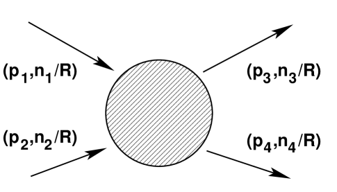
Figure 2: Momentum labeling for 5D Mandelstam variables in Eq. (3.6).

We then find that at one-loop order, the couplings $\lambda_{n_{1},n_{2},n_{3},n_{4}}$ are no longer universal; new corrections $X^{(\lambda)}_{n_{1},n_{2},n_{3},n_{4}}$ are introduced. Defining these corrections through the relation

$$\lambda_{n_{1},n_{2},n_{3},n_{4}}=\left[\lambda_{0000}+\frac{\lambda^{2}}{4\pi}X^{(\lambda)}_{n_{1},n_{2},n_{3},n_{4}}\right]\,\delta_{n_{1}+n_{2}-n_{3}-n_{4},0}~{},$$ (3.7)

we find that they each receive three contributions:

$$X^{(\lambda)}_{n_{1},n_{2},n_{3},n_{4}}~{}=~{}\xi_{n_{1}+n_{2}}(s)+\xi_{n_{1}-n_{3}}(t)+\xi_{n_{1}-n_{4}}(u)~{}.$$ (3.8)

These three contributions correspond to the diagrams in Figs. 1(b), 1(c), and 1(d) respectively. Unlike $X^{(\lambda)}$ itself, the $\xi$-functions depend on only a single KK index and a single Mandelstam variable; they can thus be expressed in the form in Eq. (2.5). Using the techniques discussed in Refs. [1, 2], we then find that the corresponding $\alpha$-functions are given by

$$\xi_{n}(s):~{}~{}~{}~{}~{}~{}~{}~{}\cases{{\displaystyle\alpha_{n}(r,v,j;s)~{}=~{}\frac{1}{4\pi}\log[(r-v)^{2}+\mathcal{M}^{2}((v+j)/|n|;s)R^{2}]}~{}&\cr~{}&\cr{\displaystyle\alpha_{0}(r,v;s)~{}=~{}\frac{1}{4\pi}\log[r^{2}+\mathcal{M}^{2}(v;s)R^{2}]}~{}&\cr}$$ (3.9)

where

$$\mathcal{M}^{2}(x;s)~{}\equiv~{}x(x-1)s+m^{2}~{}.$$ (3.10)

For notational simplicity throughout the rest of this paper, we shall henceforth define

$$y_{n}~{}\equiv~{}\cases{v&for $n=0$\cr(v+j)/|n|&for $n\not=0$\cr}$$ (3.11)

and

$$\rho_{n}~{}\equiv~{}\cases{r&for $n=0$\cr r-v&for $n\not=0$~{}.\cr}$$ (3.12)

We can then simply write our result in the compact form

$$\alpha_{n}~{}=~{}\frac{1}{4\pi}\log[\rho_{n}^{2}+\mathcal{M}^{2}(y_{n};s)R^{2}]~{}.$$ (3.13)

These results are completely general. However, in order to evaluate these results numerically, it is necessary to choose specific values for the kinematic Mandelstam variables $(s,t,u)$. At first glance, one might be tempted to impose the sorts of renormalization conditions that would apply to processes involving only zero-mode fields, such as $s=4m^{2}$ and $t=u=0$. However, such conditions correspond to situations in which all of the modes have vanishing spatial momenta, and thus cannot accommodate the sorts of processes which are of interest to us, such as those involving the production of excited KK modes. Similarly, one might consider a renormalization condition such as $s=t=u=-\mu^{2}$, where $\mu$ is the floating energy scale associated with an experiment. However, these conditions cannot be satisfied when any of the incoming or outgoing particles are on shell.

We shall therefore adopt renormalization conditions of the form

$$s~{}=~{}\mu^{2}+4m^{2}~{},~{}~{}~{}~{}~{}~{}t~{}=~{}u~{}=~{}-\mu^{2}/2~{}.$$ (3.14)

Note that in the center-of-mass frame (defined as that frame in which all spatial components of the total five-momentum of the system vanish), we may identify the energy scale $\mu$ as

$$\mu^{2}~{}=~{}4(\vec{p}^{\,2}+p_{5}^{2})$$ (3.15)

where $\vec{p}$ and $p_{5}$ are the spatial momentum components of any single particle alone. (Of course, in this center-of-mass frame, the assigned KK mode-numbers $n\sim Rp_{5}$ of these states might differ from those we have been assigning in our four-dimensional “lab” frame.) However, despite the somewhat intuitive form of the renormalization conditions in Eq. (3.14), it is important to realize that these conditions place special restrictions on the scattering angle. Such restrictions are unfortunately unavoidable, and will arise for any such constraint on the three Mandelstam variables.

In Fig. 3, we plot the difference between the one-loop $\lambda_{0,0,1,-1}$ coupling and the one-loop $\lambda_{0000}$ coupling as a function of $\mu$. This difference, of course, would have been zero at tree level, and reflects the breaking of 5D Lorentz invariance that appears at one-loop order in this theory. Note that $\lambda_{0,0,1,-1}$ is the coupling which governs the process by which two zero-mode states scatter/annihilate to produce two lowest-lying excited KK states. As we see from Fig. 3, one-loop effects cause $\lambda_{0,0,1,-1}$ to become larger than $\lambda_{0000}$. This implies that there is a small enhancement of the coupling between the zero mode and the first-excited KK mode relative to the couplings amongst the zero modes themselves. Although this enhancement is extremely small, we see from Fig. 3 that it is largest precisely at the threshold for the production of the first-excited mode, falling significantly as $\mu$ increases. We also observe that this enhancement decreases as the five-dimensional scalar mass $m$ increases, and ultimately vanishes as $m\to\infty$.

Figure 3: One-loop enhancement of the coupling $\lambda_{0,0,1,-1}$ for the production of the lowest-lying excited KK states. We plot $\Delta\lambda\equiv X_{0,0,1,-1}=(\lambda_{0,0,1,-1}-\lambda_{0000})/\chi$ as a function of the energy scale $\mu R$, where $\chi\equiv\lambda_{0000}^{2}/4\pi$. Curves A, B, and C respectively represent the cases with $m^{2}R^{2}=\{0,0.25,0.5\}$. As always, the four incoming and outgoing KK modes are taken to be on shell, and the scale $\mu$ is defined according to the conditions in Eq. (3.14). Note that in this plot, the scale $\mu$ runs from the $(n_{3},n_{4})=(1,-1)$ threshold energy at which the lowest-lying excited KK states can be produced to the $(n_{3},n_{4})=(2,-2)$ threshold energy at which the second-lowest excited states can be produced. We observe that in general, these radiative corrections are greater for smaller five-dimensional masses $m$ and decrease as functions of $\mu$.

It is clear from this plot that the one-loop coupling corrections in the $\lambda\phi^{4}$ theory are exceedingly small. However, we shall see that the analogous corrections in Yukawa theory will be significantly larger.

Finally, we observe that for certain values of $s$, the function $\alpha_{n}^{(\xi)}(s)$ in Eq. (3.9) can be complex. Although the imaginary part of an amplitude can be important, only the real part of an amplitude plays a role in the renormalization of Lagrangian parameters such as masses and couplings. Therefore, unless explicitly stated otherwise, it is to be understood throughout the remainder of this paper that we are implicitly taking the real part of any expression which describes the magnitude of a radiative correction for any KK parameter.

4 Yukawa theory

We now turn to the case of 5D Yukawa theory in which a scalar particle interacts with a Dirac fermion. In some sense, this is the next-simplest theory to consider. Moreover, as we shall see, the structure of the radiative corrections is far more intricate, both for the KK masses and for the couplings.

For Yukawa theory, we will consider two cases: one in which the scalar is real, and the other in which it is complex. In the case of a real scalar, we shall take the 5D action to be

$$S=\int d^{4}x\int_{0}^{2\pi R}dy\left[{\textstyle{1\over 2}}\partial_{M}\phi\partial^{M}\phi-{\textstyle{1\over 2}}m_{\phi}^{2}\phi^{2}+\bar{\psi}(i\gamma^{M}\partial_{M}-m_{\psi})\psi-G\phi\bar{\psi}\psi\right]$$ (4.1)

where $\phi$ and $\psi$ respectively denote the scalar and Dirac fermion (with five-dimensional masses $m_{\phi}$ and $m_{\psi}$ respectively) and where $G$ is the Yukawa coupling between the two. In the case of a complex scalar, by contrast, our action is slightly modified:

$$S=\int d^{4}x\int_{0}^{2\pi R}dy\left[{\textstyle{1\over 2}}\partial_{M}\phi^{*}\partial^{M}\phi-{\textstyle{1\over 2}}m_{\phi}^{2}\phi^{*}\phi+\bar{\psi}(i\gamma^{M}\partial_{M}-m_{\psi})\psi-G(\phi\bar{\psi}\psi+{\rm h.c.})\right]~{}.$$ (4.2)

As we shall see, these two cases lead to somewhat different results. Note that in both cases, our gamma-matrices take the form $\gamma^{M}\equiv(\gamma^{\mu},\tilde{\gamma}^{5})$ where $\tilde{\gamma}^{5}\equiv i\gamma^{5}=-\gamma^{0}\gamma^{1}\gamma^{2}\gamma^{3}$.

Performing the KK reduction of this theory is relatively straightforward. We first consider the case in which $\phi$ is real. The KK decomposition of the scalar is again given by Eq. (3.2), while the KK decomposition of the fermion takes the analogous form:

$$\psi(x^{\mu},y)~{}=~{}\frac{1}{\sqrt{2\pi R}}\,\sum_{n\in\mathchoice{\hbox{\cmss Z\kern-3.99994ptZ}}{\hbox{\cmss Z\kern-3.99994ptZ}}{\lower 0.9pt\hbox{\cmsss Z\kern-2.79996ptZ}}{\lower 1.2pt\hbox{\cmsss Z\kern-2.79996ptZ}}}\,\psi_{n}(x^{\mu})\,e^{iny/R}~{}.$$ (4.3)

We then obtain the effective four-dimensional action

$$S = \int d^{4}x\biggl{[}{\textstyle{1\over 2}}\sum_{n}\partial_{\mu}\phi_{n}^{\ast}\partial^{\mu}\phi_{n}~{}+~{}\sum_{n}\overline{\psi}_{n}i\gamma^{\mu}\partial_{\mu}\psi_{n}~{}-~{}{\textstyle{1\over 2}}\sum_{n}m_{\phi n}^{2}\phi^{\ast}_{n}\phi_{n}$$ (4.4)

$$~{}~{}~{}~{}~{}~{}~{}~{}-~{}\sum_{n}\overline{\psi}_{n}m_{\psi n}\psi_{n}~{}-~{}\sum_{n}\sum_{n^{\prime}}\,\phi_{n^{\prime}-n}\,\overline{\psi}_{n^{\prime}}\,\hat{g}_{n,n^{\prime}}\,\psi_{n}~{}+~{}...\biggr{]}~{}$$

where the tree-level boson masses are given by

$$m_{\phi n}^{2}~{}=~{}m_{\phi}^{2}+{n^{2}\over R^{2}}~{}$$ (4.5)

and where the fermion masses $m_{\psi n}$ and couplings $\hat{g}_{n,n^{\prime}}$ are matrices in spinor space, each with a “vector” or “Dirac” part (proportional to the identity in spinor space) and an “axial” part (proportional to $\gamma^{5}$):

$$m_{\psi n} = m_{\psi n}^{(D)}-im_{\psi n}^{(A)}\gamma^{5}$$

$$\hat{g}_{n,n^{\prime}} = g_{n,n^{\prime}}^{(D)}+ig_{n,n^{\prime}}^{(A)}\,\gamma^{5}~{}$$ (4.6)

with tree-level values given by

$$\cases{m_{\psi n}^{(D)}=m_{\psi}~{},~{}~{}~{}~{}m_{\psi n}^{(A)}=n/R&{}\cr g_{n,n^{\prime}}^{(D)}=G/\sqrt{2\pi R}\equiv g~{},~{}~{}~{}g_{n,n^{\prime}}^{(A)}=0~{}.&{}\cr}$$ (4.7)

Note that the axial part of the boson/fermion coupling vanishes at tree level.

The situation is nearly identical for a complex scalar field. Following the same Kaluza-Klein reduction results in a four-dimensional action of the form in Eq. (4.4) except that we no longer identify $\phi^{\ast}_{n}$ with $\phi_{-n}$, and we replace $\phi_{r^{\prime}-r}\to\phi_{r^{\prime}-r}+\phi^{\ast}_{r-r^{\prime}}$ in the final coupling term.

It may seem, at first glance, that the appearance of the “axial” $\gamma^{5}$-terms in the four-dimensional action violates four-dimensional parity symmetry. However, it turns out that all terms which are proportional to $\gamma_{5}$ will also be odd with respect to $n\to-n$. As a result, parity will actually be conserved at all energy scales. This, of course, is ultimately a reflection of underyling five-dimensional symmetries. Indeed, while $\gamma_{5}$ is odd under the four-dimensional P and CP symmetries, the quantity $n$ is actually proportional to the momentum component along the fifth dimension. Thus the quantity $n$ is “odd” under P, thereby making the product $\gamma_{5}n$ even, as required.

We see, then, that there are five quantities in KK-reduced 5D Yukawa theory which are capable of receiving radiative corrections: $m_{\phi n}$, $m_{\psi n}^{(D)}$, $m_{\psi n}^{(A)}$, $g_{n,n^{\prime}}^{(D)}$, and $g_{n,n^{\prime}}^{(A)}$. We shall now explore the one-loop corrections to each of these in turn.

4.1 Boson KK mass corrections

Regardless of whether the 5D scalar is real or complex, we shall parametrize the one-loop corrections to the KK boson masses $m_{\phi n}$ in the form

$$m_{\phi n}^{2}~{}=~{}m_{\phi 0}^{2}+\frac{n^{2}}{R^{2}}+\frac{g^{2}}{4\pi R^{2}}\,X_{n}^{(m_{\phi}^{2})}~{}$$ (4.8)

where $g$ is the universal tree-level coupling in Eq. (4.7), as appropriate for a calculation of this order. Using the techniques developed in Refs. [1, 2], we then find that the corresponding functions $\alpha_{n}$ are given by

$$\alpha_{n}(r,v,j) = \frac{1}{\pi}\biggl{\{}\left[\rho_{n}^{2}+(1-2y_{n})|n|\rho_{n}\right]\,\log(\rho_{n}^{2})$$

$$-\left[\rho_{n}^{2}+(1-2y_{n})|n|\rho_{n}+3\mathcal{M}_{\phi}^{2}(y_{n};m_{\phi}^{2})R^{2}\right]\,\log(\rho_{n}^{2}+\mathcal{M}_{\phi}^{2}(y_{n};m_{\phi}^{2})R^{2})\biggr{\}}$$

where $y_{n}$ and $\rho_{n}$ are respectively defined in Eqs. (3.11) and (3.12) and where

$$\mathcal{M}_{\phi}^{2}(y;m_{\phi}^{2})~{}=~{}m_{\psi}^{2}+y(y-1)m_{\phi}^{2}~{}.$$ (4.10)

This compact result contains a wealth of information. One important feature is the behavior of $X_{1}^{(m_{\phi}^{2})}$ — i.e., the radiative correction to the mass of the first-excited KK boson relative to the mass of the KK zero mode — as a function of the two five-dimensional masses in our problem, $m_{\phi}$ and $m_{\psi}$. This behavior is shown in Fig. 4, where $X_{1}^{(m_{\phi}^{2})}$ is plotted as a function of $m_{\psi}$ for three different “benchmark” values of $m_{\phi}$. Several features are immediately apparent:

• $X_{1}^{(m_{\phi}^{2})}=0$ for $m_{\phi}=m_{\psi}=0$. We shall see, in fact, that this is a general phenomenon for all $X_{n}^{(m_{\phi}^{2})}$.

• $X_{1}^{(m_{\phi}^{2})}$ is negative when $m_{\psi}=0$ and $m_{\phi}\not=0$. This means that the mass splitting between the first-excited KK boson mode and the KK zero mode is reduced by one-loop radiative corrections — i.e., these two states begin to approach each other. Moreover, the magnitude of this effect increases with increasing $m_{\phi}$.

• $X_{1}^{(m_{\phi}^{2})}\to 0$ as $m_{\psi}\to\infty$ for all $m_{\phi}$. This occurs because the functions $\alpha_{n}$ and $\alpha_{0}$ in Eq. (LABEL:phn) approach each other in this limit. There is therefore no difference in this limit between the corrections to the masses of the KK zero mode and first-excited mode — i.e., in this limit the tree-level mass spacing between the zero mode and first excited mode is preserved to one-loop order.

• $X_{1}^{(m_{\phi}^{2})}$ is generally non-monotonic as a function of $m_{\psi}$. For $m_{\phi}$ above a critical value, $X_{1}^{(m_{\phi}^{2})}$ actually reaches a positive maximum for a value of $m_{\psi}$ which increases with $m_{\phi}$. This non-monotonic behavior emerges as the result of a competition between the corrections to the mass of the first-excited KK mode and the corrections to the mass of the KK zero mode. Indeed, each of these corrections is individually monotonic.

• Finally, although it may be somewhat difficult to observe in Fig. 4, it turns out that $X_{1}^{(m_{\phi}^{2})}$ actually experiences a kink (i.e., a slight discontinuous change in slope) as a function of $m_{\psi}$ prior to reaching its maximum value. Indeed, this occurs for all $m_{\phi}>0$. These kinks mark the thresholds for the decays of either the KK boson zero mode or the KK first-excited mode. Indeed, these thresholds correspond to values of $m_{\psi}$ at which the imaginary parts of the diagrams which renormalize the scalar masses become zero.

           

Figure 4: The relative one-loop boson mass corrections $X_{1}^{(m_{\phi}^{2})}$ between the first-excited KK boson mode and the KK zero mode, plotted as functions of $m_{\psi}$ for different values of $m_{\phi}$.

           

Figure 5: The relative one-loop corrections $X_{n}^{(m_{\phi}^{2})}$ for the KK boson squared masses, plotted as functions of $n$ for different values of $m_{\phi}$. In each plot, Curves A, B, and C represent the cases with $m_{\psi}^{2}R^{2}=\{0,0.25,0.5\}$ respectively — a naming scheme that will continue to hold for all remaining figures in this paper.

We can also examine $X_{n}^{(m_{\phi}^{2})}$ as functions of $n$. This behavior is shown in Fig. 5 for different values of $m_{\phi}$ and $m_{\psi}$. Once again, certain features are readily apparent:

• For $m_{\phi}=m_{\psi}=0$, we find that $X_{n}^{(m_{\phi}^{2})}=0$ for all $n\geq 0$. This is therefore an example of Case #1 from the Introduction: the tree-level form of the KK mass relation for the bosonic fields is preserved at one loop. We thus see that it is only the presence of a non-zero five-dimensional mass, either $m_{\phi}$ or $m_{\psi}$, which breaks the apparent 5D Lorentz invariance as far as the tree-level bosonic spectrum is concerned.

• For $m_{\phi}=0$ and $m_{\psi}\not=0$, we find that $X_{n}^{(m_{\phi}^{2})}=$ constant as a function of $n$. In fact, this constant depends on $m_{\psi}$ in a non-monotonic way, hitting zero only for $m_{\psi}=0$ (as discussed in the previous case). This is therefore an example of Case #3a from the Introduction: all excited KK modes have masses which shift uniformly relative to that of the KK zero mode. Thus, all KK modes continue to obey the tree-level mass relation except for the zero mode.

• For $m_{\phi}\not=0$, we find that $X_{n}^{(m_{\phi}^{2})}$ increases with $n$ but quicky reaches a non-zero asymptote as $n\to\infty$. This is therefore an example of Case #3b, but with a behavior resembling that of Case #3a for the uppermost portions of the KK tower.

It should come as no surprise that the radiative corrections to KK masses are generically of the form given in Case #3a when $n\to\infty$ — i.e., that they become independent of $n$ as $n\to\infty$. The limit of large KK mode numbers corresponds to high momentum components along the extra dimension, and the discretization of momentum that arises due to compactification becomes negligible in this limit. We therefore expect that the limit of high KK mode numbers should correspond to an uncompactified theory in which the tree-level KK dispersion relation holds (signifying the restoration of a full 5D Lorentz invariance). By contrast, the lower portions of the KK tower are more sensitive to the discretization of the momentum in the compactified dimension. Thus the upper portions of the KK tower have approximately equal mass-squared spacings relative to each other, but this pattern does not hold all the way down to the zero mode.

It is also instructive to see how this asymptotic behavior of equal spacings emerges analytically. Towards this end, we can use the $\alpha_{n}$-functions in Eq. (LABEL:phn) in order to calculate the contribution to $X_{n}^{(m_{\phi}^{2})}$ from states with a fixed mode number $n^{\prime}$. For simplicitly, we shall assume that $n^{\prime}\gg n$, and likewise we shall assume that $n^{\prime}$ is chosen sufficiently large that $\Lambda\gg m_{\phi},m_{\psi}$ where $\Lambda\equiv n^{\prime}/R$. We can then expand this contribution in powers of $m/\Lambda$ where $m$ denotes either $m_{\phi}$ or $m_{\psi}$, and we find that this expansion takes the form

$$\frac{g^{2}}{4\pi^{2}}\Biggl{\{}\left(\frac{7m_{\psi}^{2}-m_{\phi}^{2}}{3}\right){1\over\Lambda^{2}}$$

$$~{}~{}~{}+\Biggl{[}\frac{9m_{\psi}^{2}-m_{\phi}^{2}}{10R^{2}}-\frac{11m_{\psi}^{4}}{2}+\frac{1}{6}\left(-1+\frac{1}{10n^{2}}\right)m_{\phi}^{4}+\frac{1}{3}\left(5-\frac{1}{5n^{2}}\right)m_{\psi}^{2}m_{\phi}^{2}\Bigg{]}\frac{1}{\Lambda^{4}}$$

$$~{}~{}~{}+\mathcal{O}(m^{6}/\Lambda^{6})\Biggr{\}}~{}.$$ (4.11)

Although we have made no assumptions about the size of $n$ itself, we see that each coefficient in our expansion depends on $n$ only through negative powers. This is ultimately the source of the fact that our total mass corrections exhibit a finite, asymptotic limit as $n\to\infty$. Indeed, although the results in Eq. (4.11) hold only for very large $n^{\prime}$, it turns out that the behavior illustrated in these results is in fact completely general, and holds even for smaller values of $n^{\prime}$ as well.

4.2 Fermion KK mass corrections

We now turn to the renormalized masses of the KK fermion modes. Recall from Eq. (4.7) that these masses contain both a vector (or “Dirac”) component $m_{\psi}^{(D)}$ and an axial component $m_{\psi}^{(A)}$. Parametrizing the one-loop corrections to these masses in the form

$$m_{\psi n}^{(D)} = m_{\psi 0}^{(D)}+\frac{g^{2}}{4\pi R}X_{n}^{(m_{\psi}^{(D)})}$$

$$m_{\psi n}^{(A)} = \frac{n}{R}+\frac{g^{2}}{4\pi R}X_{n}^{(m_{\psi}^{(A)})}~{},$$ (4.12)

we find that the corresponding $\alpha_{n}$-functions take the forms

$$X_{n}^{(m_{\psi}^{(D)})}:~{}~{} \alpha^{(\psi D)}_{n}~{}=~{}\frac{m_{\psi}R}{4\pi}(1+y_{n})\log(\rho_{n}^{2}+\mathcal{M}_{\psi}^{2}(y_{n})R^{2})$$

$$X_{n}^{(m_{\psi}^{(A)})}:~{}~{} \alpha^{(\psi A)}_{n}~{}=~{}\frac{{\rm sign}\/(n)}{4\pi}\rho_{n}\left[\log(\rho_{n}^{2}+\mathcal{M}_{\psi}^{2}(y_{n})R^{2})-\log(\rho_{n}^{2})\right]~{}$$ (4.13)

where

$$\mathcal{M}_{\psi}^{2}(y)~{}\equiv~{}(y-1)^{2}m_{\psi}^{2}+ym_{\phi}^{2}~{}.$$ (4.14)

The variables $y_{n}$ and $\rho_{n}$ were defined in Eqs. (3.11) and (3.12) respectively. While these results apply if the five-dimensional scalar $\phi$ is real, promoting the 5D scalar to a complex field merely doubles the values of both of the $\alpha_{n}$-functions. Note that the quantity ${\rm sign}\/(n)$ in Eq. (4.13) is taken to be zero when $n=0$, as a consequence of which the function $\alpha^{(\psi A)}_{0}$ vanishes.

The results in Eq. (4.13) describe the corrections to the masses of the fermion KK modes. However, for the sake of comparison with our results for the boson KK modes, it will actually be more appropriate to consider the corresponding corrections to the squared masses of the fermion KK modes. However, given the parametrizations in Eq. (4.12), we immediately see that

$$m_{\psi n}^{(D)2} = m_{\psi 0}^{(D)2}+\frac{g^{2}}{4\pi R^{2}}Y_{n}^{(m_{\psi}^{(D)})}+{1\over R^{2}}{\cal O}(g^{4})$$

$$m_{\psi n}^{(A)2} = \frac{n^{2}}{R^{2}}+\frac{g^{2}}{4\pi R^{2}}Y_{n}^{(m_{\psi}^{(A)})}+{1\over R^{2}}{\cal O}(g^{4})~{},$$ (4.15)

where the corrections to the squared masses are given to lowest order in $g$ by

$$Y_{n}^{(m_{\psi}^{(D)})}~{}=~{}2m_{\psi 0}^{(D)}R\,X_{n}^{(m_{\psi}^{(D)})}~{},~{}~{}~{}~{}~{}Y_{n}^{(m_{\psi}^{(A)})}~{}=~{}2n\,X_{n}^{(m_{\psi}^{(A)})}~{}.$$ (4.16)

Indeed, retaining higher orders in $g$ would be incorrect since additional contributions at such orders would also come from two-loop diagrams, which we have been neglecting.

           

Figure 6: The relative one-loop corrections $Y_{n}^{(m_{\psi}^{(D)})}$ for the KK fermion squared Dirac masses, plotted as functions of $n$ for different values of $m_{\phi}$ and $m_{\psi}$.

           

Figure 7: The relative one-loop corrections $Y_{n}^{(m_{\psi}^{(A)})}$ for the KK fermion squared axial masses, plotted as functions of $n$ for different values of $m_{\phi}$ and $m_{\psi}$.

     

Figure 8: The relative one-loop correction $X_{1}^{(m_{\psi}^{(A)})}$ to the linear axial mass of the first excited KK fermion, plotted versus $\Delta m^{2}$ for fixed values of $m^{2}$. The quantities $m^{2}$ and $\Delta m^{2}$ are defined such that $m_{\psi}^{2}=m^{2}-\Delta m^{2}$, and $m_{\phi}^{2}=m^{2}+\Delta m^{2}$. As in Fig. 7, we see that these corrections are positive if $m_{\phi}>m_{\psi}$, negative if $m_{\phi}<m_{\psi}$, and zero if $m_{\phi}=m_{\psi}$.

           

Figure 9: The relative one-loop corrections $Y_{n}^{(m_{\psi})}$ for the physical KK fermion masses, plotted as functions of $n$ for different values of $m_{\phi}$ and $m_{\psi}$.

The corrections to the squared Dirac masses are shown in Fig. 6. Likewise, corrections to the squared axial masses are shown in Fig. 7. As we observe from these figures, the Dirac and axial mass corrections do exhibit certain common behaviors. For example, in both cases these corrections are monotonic with mode number $n$, and they each approach constant values as $n\to\infty$.

However, there are also certain crucial differences between the behaviors of the Dirac and axial mass corrections. The Dirac corrections, for example, vanish if $m_{\psi}=0$ (regardless of the value of $m_{\phi}$); thus it is the fermion bare mass $m_{\psi}$ which is responsible for triggering a non-zero one-loop mass correction. Likewise, the Dirac corrections are positive and increase as functions of $m_{\psi}$, while they generally decrease as functions of $m_{\phi}$ (with $m_{\psi}$ held fixed).

By contrast, the axial mass corrections are positive if $m_{\phi}>m_{\psi}$, negative if $m_{\psi}<m_{\phi}$, and zero if $m_{\psi}=m_{\phi}$. Indeed, the behavior of the correction $X_{1}^{(m_{\psi}^{(A)})}$ to the linear axial mass of the first-excited KK fermionic state is shown in Fig. 8 as a function of the difference $m_{\phi}^{2}-m_{\psi}^{2}$, and we see that this function is positive when this difference is positive, negative when this difference is negative, and zero precisely when this difference is zero.

It is an interesting phenomenon that the axial mass corrections vanish for $m_{\psi}=m_{\phi}$. It is straightforward to demonstrate this explicitly at one-loop order using the expressions for the mass corrections given above, and one finds that this results from a cancellation between the effects of the different KK boson and fermion propagators in the loop. This suggests a possible supersymmetric origin for this cancellation, and indeed we observe that although the Yukawa theory under study here is not supersymmetric, the one-loop corrections to the fermion masses in this Yukawa theory are equivalent (up to an overall multiplicative constant) to the corresponding corrections in a supersymmetric Yukawa theory, provided $m_{\psi}=m_{\phi}$. This is significant because supersymmetry forbids KK fermions from accruing axial mass corrections.

Finally, we observe that the corrections to the axial fermion masses $m_{\psi n}^{(A)}$ are also odd functions of the mode number $n$. Although this is not evident from the plots in Fig. 7, this result follows directly as the consequence of the analytic expression for the axial mass correction given in Eq. (4.13): the prefactor ${\rm sign}(n)$ is odd under $n\to-n$, while the rest of the expression is manifestly even under $n\to-n$. This property is a direct consequence of the overall P and CP symmetries of our original five-dimensional theory. As a corollary, this symmetry protects the fermion zero mode from gaining an axial mass.

Thus far, we have discussed the corrections to the individual Dirac and axial components of the KK fermion masses. However, for many purposes the important quantities are actually the total physical fermionic masses themselves — i.e., the masses corresponding to the poles in the KK fermion propagators. In general, the squares of these masses are the sums of the squares of the two individual mass components:

$$m_{\psi n}^{2}~{}\equiv~{}m_{n\psi}^{\dagger}m_{n\psi}~{}=~{}m_{\psi n}^{(D)2}+m_{\psi n}^{(A)2}~{},$$ (4.17)

where $m_{\psi n}$ is the fermion mass given in Eq. (4.6). It then follows from Eq. (4.15) that the corrections to this mass take the form

$$m_{\psi n}^{2}~{}=~{}m_{\psi 0}^{2}+\frac{n^{2}}{R^{2}}+\frac{g^{2}}{4\pi R^{2}}Y_{n}^{(m_{\psi})}+{1\over R^{2}}{\cal O}(g^{4})~{}$$ (4.18)

where we have recognized $m_{\psi 0}^{2}=m_{\psi 0}^{(D)2}+{\cal O}(g^{4})/R^{2}$ and where

$$Y_{n}^{(m_{\psi})}~{}\equiv~{}Y_{n}^{(m_{\psi}^{(D)})}+Y_{n}^{(m_{\psi}^{(A)})}~{}.$$ (4.19)

These corrections are shown in Fig. 9.

Unlike the individual corrections to the Dirac and axial mass components, these overall corrections do not behave as simple monotonic functions of the bare masses $m_{\phi}$ and $m_{\psi}$. This non-trivial behavior ultimately arises as the result of a competition between the contributions from the Dirac and axial corrections in Eq. (4.17). Indeed, as evident in Figs. 6 and 7, these corrections to the squared Dirac and axial masses vary in opposite directions with respect to the fermion bare mass. We also observe that these corrections are also generally largest when $m_{\phi}=0$. This enhancement arises due to the fact that the logarithms in the Dirac and axial corrections become large when their arguments tend to zero. We nevertheless see that these corrections all approach constant values as $n\to\infty$, indicating that the the uppermost portions of the KK tower effectively behave according to Case #3a from the Introduction. We also observe that these corrections vanish only when $m_{\phi}=m_{\psi}=0$. This is then an example of Case #1.

4.3 Yukawa coupling corrections

Finally, we consider the one-loop corrections to the Yukawa coupling. Like the coupling in the $\lambda\phi^{4}$ theory discussed in Sect. 3, we shall express the Yukawa coupling and its one-loop corrections as functions of a canonical (non-Wilsonian) renormalization scale $\mu$, which we shall here take to be the squared five-momentum of the scalar mode (i.e., $\mu^{2}=-Q^{2}$ where $Q^{M}$ is the scalar five-momentum). This in some sense defines the energy of the experiment through which this coupling is measured. However, unlike the case of $\lambda\phi^{4}$ theory, the results for the one-loop coupling corrections here are more complicated due to several factors, including the presence of non-zero field-strength renormalizations and the existence of relevant Feynman diagrams involving more than a single Feynman parameter. Neither of these features appeared in the $\lambda\phi^{4}$ theory at one-loop order. Moreover, as indicated in Eq. (4.6), the Yukawa coupling actually has two independent components, one “vector” (or Dirac) and the other axial.

Despite these complications, we can parametrize the one-loop corrections to these Yukawa coupling components in the form

$$g_{n_{1},n_{2}}^{(D)} = g_{00}^{(D)}+{g^{3}\over 8\pi^{3/2}}\left[L^{(D)}_{n_{1},n_{2}}+Z^{(\phi)}_{n_{2}-n_{1}}+Z^{(\psi)}_{n_{1}}+Z^{(\psi)}_{n_{2}}\right]$$

$$g_{n_{1},n_{2}}^{(A)} = {g^{3}\over 8\pi^{3/2}}\,L^{(A)}_{n_{1},n_{2}}~{},$$ (4.20)

where $g$ is defined in Eq. (4.7). In Eq. (4.20), the quantities $Z^{(\phi,\psi)}$ represent the contributions from bosonic and fermionic field-strength renormalizations, while $L^{(D,A)}$ represent those parts of the appropriate one-loop vertex renormalization diagram which are proportional to ${\bf 1}$ and $\gamma^{5}$ respectively in spinor space. Note, in particular, that what we are denoting $Z^{(\phi,\psi)}$ are merely contributions from the field-strength renormalizations; they are not the complete renormalizations themselves. As might be expected, field-strength renormalizations yield corrections to Dirac (vector) couplings but not the axial couplings. In this connection, we observe that there were no one-loop field-strength renormalization contributions to the analogous coupling corrections in the $\lambda\phi^{4}$ case because the appropriate loop integral in the $\lambda\phi^{4}$ case was completely independent of the momentum on the external leg. This is ultimately the same reason that the KK mass relation for the $\phi$ fields in the $\lambda\phi^{4}$ theory was invariant to this order.

Given the parametrization in Eq. (4.20), our results are as follows. The field-strength renormalization contributions $Z^{(\phi,\psi)}$ take the standard form in Eq. (2.5), where the corresponding $\alpha_{n}$-functions are given by

$$Z_{n}^{(\phi)}: \alpha_{n}~{}=~{}\frac{1}{\sqrt{\pi}}\,y_{n}(1-y_{n})\Bigg{[}3\log\left(\rho_{n}^{2}+\mathcal{M}^{2}_{\phi}(y_{n};\mu^{2})R^{2}\right)$$

$$~{}~{}~{}~{}~{}~{}~{}~{}~{}~{}~{}~{}~{}~{}~{}~{}~{}~{}~{}~{}~{}~{}~{}+\frac{(1-2y_{n})|n|\rho_{n}+2\mathcal{M}^{2}_{\phi}(y_{n};\mu^{2})R^{2}}{\rho_{n}^{2}+\mathcal{M}^{2}_{\phi}(y_{n};\mu^{2})R^{2}}\Bigg{]}~{}$$

$$Z_{n}^{(\psi)}: \alpha_{n}~{}=~{}\frac{1}{4\sqrt{\pi}}\,y_{n}\left[\log\left(\rho_{n}^{2}+\mathcal{M}^{2}_{\psi}(y_{n})R^{2}\right)+\frac{2(y_{n}^{2}-1)m_{\psi}^{2}R^{2}}{\rho_{n}^{2}+\mathcal{M}^{2}_{\psi}(y_{n})R^{2}}\right]~{}.$$ (4.21)

Note that the quantities $y_{n}$, $\rho_{n}$, $\mathcal{M}^{2}_{\phi}$, and $\mathcal{M}^{2}_{\psi}$ are defined in Eqs. (3.11), (3.12), (4.10), and (4.14) respectively. Also note that on-shell renormalization conditions for $Z^{(\psi)}$ have been applied in obtaining Eq. (4.21).

The situation is significantly more complex for the contributions $L^{(D,A)}$ coming from the vertex renormalizations because the relevant diagrams in this case involve two Feynman parameters rather than just one. However, it turns out that there does exist a simple closed form for these corrections which is analogous to that in Eq. (2.5) when either $n_{1}$ or $n_{2}$ is zero. For concreteness, let us assume that $n_{2}$ is zero. In such cases, Eq. (2.5) is replaced by

$$L_{n_{1},0}~{}=~{}\sum_{r=-\infty}^{\infty}\frac{1}{|n_{1}|}\sum_{j=0}^{|n_{1}|-1}\int_{0}^{1}dv_{1}\int_{0}^{1}dv_{2}\,\Big{[}\alpha_{n_{1},0}(r,v_{1},v_{2},j)-\alpha_{0,0}(r,v_{1},v_{2})\Big{]}~{}.$$ (4.22)

We then find that the corresponding $\alpha_{n_{1},0}$-functions are given by

$$L_{n_{1},0}^{(D)}: \alpha_{n_{1},0}~{}=~{}\frac{1}{\sqrt{\pi}}(1-y_{n_{1}})\Bigg{[}\log(\rho_{n_{1}}^{2}+\mathcal{M}^{2}_{g}(y_{n_{1}},y_{0}^{\prime};\mu^{2})R^{2})$$

$$~{}~{}~{}~{}~{}~{}~{}~{}~{}~{}~{}~{}~{}~{}~{}~{}~{}~{}~{}~{}+\frac{1}{2}\,\frac{\mathcal{M}_{g}^{2}(y_{n_{1}},y_{0}^{\prime};\mu^{2})R^{2}+(2-v_{1}-v_{2})^{2}m_{\psi}^{2}R^{2}}{\rho_{n_{1}}^{2}+\mathcal{M}_{g}^{2}(y_{n_{1}},y^{\prime}_{0};\mu^{2})R^{2}}\Bigg{]}$$

$$L_{n_{1},0}^{(A)}: \alpha_{n_{1},0}~{}=~{}-\frac{1}{\sqrt{\pi}}(1-y_{n_{1}})(2-y_{n_{1}}-y_{0}^{\prime})\,\frac{\rho_{n_{1}}\,m_{\psi}R}{\rho_{n_{1}}^{2}+\mathcal{M}_{g}^{2}(y_{n_{1}},y^{\prime}_{0};\mu^{2})R^{2}}~{},$$

where $y_{n}$ and $\rho_{n}$ are defined as in Eqs. (3.11) and (3.12) except with $v$ replaced by $v_{1}$, where $y_{0}^{\prime}\equiv v_{2}(1-y_{n_{1}})$, and where

$$\mathcal{M}^{2}_{g}(y,y^{\prime};\mu^{2})~{}\equiv~{}(y+y^{\prime})^{2}m_{\psi}^{2}+(1-y-y^{\prime})m_{\phi}^{2}-yy^{\prime}\mu^{2}~{}.$$ (4.24)

The above expressions for the $\alpha$-functions assume that $n_{1}\not=0$ and $n_{2}=0$. However, analogous results exist when $n_{1}=0$ and $n_{2}\not=0$. Likewise, the results listed above apply when the 5D scalar in our theory is real. When this field is complex, by contrast, the $\alpha$-functions corresponding to the $Z^{(\psi)}$ and $L^{(D,A)}$ corrections double, while the $\alpha$-function corresponding to the $Z^{(\phi)}$ correction remains invariant.

In Fig. 11 we plot the energy dependence of the total one-loop correction to the coupling component $g_{1,0}^{(D)}$ which governs the production of a pair of first-excited KK fermion modes via the $t$-channel interaction shown in Fig. 11 between two incoming zero-mode fermions. Note, in this connection, that $g_{0,1}^{(D)}=g_{0,-1}^{(D)}=g_{1,0}^{(D)}=g_{-1,0}^{(D)}$. Relative to the corrections to the zero-mode couplings, these KK-production couplings can be either positive or negative, depending on the energy scale and the values of the bare masses. As a result, we see that these one-loop corrections can either enhance or suppress the amplitude for the creation of the first excited KK mode. However, unlike the analogous case shown in Fig. 3 for the coupling in the $\lambda\phi^{4}$ theory, the coupling that governs the production of excited KK fermion modes in the Yukawa theory actually increases relative to the zero-mode coupling as a function of the energy scale.

         

Figure 10: The total relative one-loop correction $L^{(D)}_{1,0}+Z^{(\phi)}_{-1}+Z^{(\psi)}_{1}+Z^{(\psi)}_{0}$ to the coupling component $g_{n_{1},0}^{(D)}$ that governs the production of the first-excited KK fermion modes, plotted as functions of $\mu R$ for different values of $m_{\phi}$ and $m_{\psi}$. The plotted range in $\mu R$ extends approximately from the threshold for producing a particle/antiparticle pair of the first-excited KK fermion mode to the threshold for producing the second, assuming the $t$-channel interaction shown in Fig. 11 between two incoming zero-mode fermions. Unlike the analogous case shown in Fig. 3 for the coupling in the $\lambda\phi^{4}$ theory, we see that the coupling that governs the production of excited KK fermion modes in the Yukawa theory actually increases relative to the zero-mode coupling as a function of the energy scale. Thus, the production of excited KK fermions is actually slightly enhanced to one-loop order in this theory.

Figure 11: Feynman diagram showing the tree-level production of two first-excited KK fermions $\psi_{\pm 1}$ via $t$-channel scattering of two zero-mode fermions $\psi_{0}$ in the Yukawa theory. Arrows indicate the routings of five-momentum according to which the KK indices indicated in this figure are assigned. The amplitude of this process is proportional to $g_{0,1}g_{0,-1}=g_{1,0}^{2}$.

Results in Fig. 11 are plotted for $(m_{\phi}R)^{2}=0.25$ and $(m_{\phi}R)^{2}=0.5$. However, when $m_{\phi}=0$, there are infrared divergences in the one-loop diagrams responsible for corrections to the zero-mode coupling. For this reason no results are plotted in this case. Needless to say, this is not an inconsistency: infrared divergences always cancel in calculations of observables, and will do so in this higher-dimensional Yukawa theory as well. Indeed, such infrared divergences also appear in the one-loop diagrams in the 4D Yukawa theory, and even in the case of full four-dimensional QED which this Yukawa theory is meant to resemble.

           

Figure 12: The total relative one-loop contribution $L^{(A)}_{1,0}$ to the axial coupling component $g_{n_{1},0}^{(A)}$, plotted as a function of $\mu R$ for different values of $m_{\phi}$ and $m_{\psi}$. As in Fig. 11, the plotted range in $\mu R$ extends approximately from the threshold for producing a particle/antiparticle pair of the first-excited KK fermion mode to the threshold for producing the second, assuming a $t$-channel interaction between two incoming zero-mode fermions.

The results shown in Fig. 11 illustrate the Dirac-component coupling $g_{1,0}^{(D)}$. By contrast, the corrections to the corresponding axial coupling $g_{1,0}^{(A)}$ are shown in Fig. 12. Unlike the Dirac coupling, we observe that the axial coupling vanishes when $m_{\psi}=0$; thus, as expected, it is the presence of non-zero $m_{\psi}$ which triggers a non-zero axial coupling at one-loop order. We also observe that this axial coupling increases monotonically as a function of $m_{\psi}$, although it decreases monotonically as a function of $m_{\phi}$. Furthermore, this coupling is a monotonically decreasing function of the energy scale $\mu$; thus, just as in the case of the $\lambda\phi^{4}$ theory, the maximum coupling correction actually occurs at the threshold for the production of the first-excited KK fermion mode.

It is important to recognize that to one-loop order, the “corrections” shown in Fig. 12 are nothing but the axial couplings themselves, since all of these axial couplings vanish at tree level. This is therefore an instance in which a one-loop correction, though small, is actually dominant. As a consequence, any process which proceeds through such an axial coupling is a direct probe of the one-loop radiative corrections we have calculated. Such a process, though suppressed, would be uniquely characterized through an axial correlation between the spin and the corresponding angular scattering amplitude.

5 Conclusions and relation to prior work

In this paper, we investigated the extent to which radiative corrections deform the expected tree-level relations between Kaluza-Klein masses and couplings in higher-dimensional interacting theories. Such calculations are surprisingly subtle because they rely intrinsically on having quantum field-theoretic regulators which preserve higher-dimensional Lorentz invariance (and higher-dimensional gauge invariance, when appropriate); otherwise the standard renormalization calculations would produce spurious, unphysical effects which would be difficult to disentangle from the bona-fide physical effects resulting spacetime compactification. Using techniques developed in Refs. [1, 2], we concentrated on two toy theories: five-dimensional $\lambda\phi^{4}$ theory and five-dimensional Yukawa theory, each with a single dimension compactified on a circle. We then studied the resulting one-loop corrections to the tree-level mass and coupling relations, and determined those situations in which these corrections exhibited a variety of special algebraic forms and behaviors as functions of the bare five-dimensional masses in these theories and the overall renormalization energy scale.

For both $\lambda\phi^{4}$ theory and Yukawa theory on a circle, we found that our KK masses can deform in a variety of different ways. In some cases, these deformations do not disturb the underlying KK mass relations between different KK modes. In such cases, therefore, the underlying five-dimensional Lorentz invariance of the KK mass spectrum appears to be preserved. In other cases, these deformations induce changes in these relations which can be interpreted as mere shifts or “renormalizations” of the underlying five-dimensional masses or the radius of the compactification circle. However, in the most general cases, these deformations result in new KK mass relations which do not exhibit the signatures normally associated with compactification on a circle.

Similar results were also found for the KK couplings: renormalization effects can induce non-trivial splittings between KK couplings which are otherwise equal at tree level. For $\lambda\phi^{4}$ theory, we found that these splittings lead to enhanced production of the first-excited KK mode. In Yukawa theory, by contrast, we found that renormalization effects can lead to either enhanced or suppressed production of the first-excited KK mode. Whether this production is ultimately enhanced or suppressed depends on the values of the underlying five-dimensional masses and the energy scale of the experiment through which it is measured.

While many of our results were expected, others were more surprising. One interesting result, for example, is the radiative generation of a $\gamma^{5}$-interaction amongst zero modes in the Yukawa theory. Indeed, such an interaction is completely absent at tree level. As we discussed in Sect. 4, this interaction does not lead to parity or CP violation, and is analogous to the axial fermion mass terms which appear in the KK Lagrangian at tree level. Another somewhat surprising result is that the corrections to the axial masses of the fermions in Yukawa theory vanish when the zero-mode masses of the boson and fermion are equal. As we briefly discussed in Sect. 4, this cancellation ultimately occurs because the one-loop corrections to fermion propagators in Yukawa theory are equivalent to those in a supersymmetric model, up to an overall multiplicative constant. Supersymmetry should forbid axial mass corrections.

Needless to say, many previous studies have focused on loop corrections in KK theories. However, most of this prior work focused on the effects induced by the excited KK states on the properties of the zero modes. For example, a relatively early calculation of the runnings of zero-mode gauge couplings appears in Ref. [3], where it was found that the higher-dimensional radiative corrections to such runnings have the potential to lead to gauge coupling unification well below the usual GUT scale. Such running can also generate fermion mass hierarchies [3]. However, the analysis of Ref. [3] focused purely on the radiative corrections to the couplings of the zero modes, and thus did not require use of regulators designed to respect higher-dimensional Lorentz or gauge symmetries. Likewise, the authors of Ref. [4] calculated gauge-coupling corrections in warped AdS₅ space. A recent study of loop effects in this geometry appears in Ref. [5].

Another type of zero-mode calculation involves the special case in which loop corrections are finite to a certain order in perturbation theory. This variety of calculation appears in Ref. [6], for example, where the authors calculated the correction to the muon magnetic moment in higher dimensions. At one-loop order, the correction was found to be finite in 5D.

There do, however, exist several studies which have examined loop effects on excited modes. For example, the authors of Ref. [7] showed that when an extra dimension is compactified to an orbifold, loop corrections lead to logarithmically divergent terms localized at the orbifold fixed points. These can take the form of new kinetic terms or coupling terms at the fixed points.

The authors of Ref. [8] calculated corrections to KK masses in five-dimensional QED and in a five-dimensional Standard Model, considering the cases in which these theories are compactified on a flat, circular universal extra dimension and on a flat $S^{1}/\mathchoice{\hbox{\cmss Z\kern-3.99994ptZ}}{\hbox{\cmss Z\kern-3.99994ptZ}}{\lower 0.9pt\hbox{\cmsss Z\kern-2.79996ptZ}}{\lower 1.2pt\hbox{\cmsss Z\kern-2.79996ptZ}}_{2}$ orbifold. For the case of compactification on a circle, they found that if zero-mode fermion masses are neglected, the photon zero mode remains massless while the excited KK photons receive mass corrections of the form

$$\Delta m_{n}^{2}~{}=~{}-\frac{e^{2}\zeta(3)}{4\pi^{4}R^{2}}~{},~{}~{}~{}~{}n\geq 1~{},$$ (5.1)

independent of the mode number $n$. Other gauge theories lead to similar results. This sort of behavior is clearly an example of Case #3a from the Introduction: the entire excited tower experiences a uniform mass shift, while gauge invariance protects the (vanishing) mass of the gauge-boson zero mode.

The authors of Ref. [8] correctly obtained this result by performing a Poisson resummation, casting KK sums into sums over winding numbers. Indeed, the use of Poisson resummations in calculations of loop corrections first appeared in Ref. [9], and it has been verified [1] that use of our regulators also reproduces the result in Eq. (5.1). At first glance, it might seem that such a Poisson-resummation technique might also apply to the calculations in this paper. Unfortunately, this is not the case because this method does not yield closed-form expressions when the zero-mode masses are non-vanishing. Indeed, as we have seen, many of our results arise precisely because of the non-vanishing nature of these masses. As a result, regulators of the type we introduced in Refs. [1] and [2] are needed for the calculations in this paper.

As an aside, we remark that there also remains the technical issue that a Poisson resummation by itself does not regularize a divergence, but merely expresses it in a different language. In Ref. [1], for example, we noted that Poisson resummation worked in Ref. [8] because the mass corrections in those calculations were finite. For the divergent case, however, we noted that one would have to calculate differences between corrections for excited modes and zero modes, analogous to the differences introduced in Refs. [1] and [2]. Of course, one might be tempted to simply subtract the contribution arising from vanishing winding number. However, this merely corresponds to the correction in a non-compactified theory, and does not relate directly to observables in the compactified theory.

The authors of Ref. [10] calculated loop corrections to KK gauge-boson masses using a mixed propagator. In this approach, the four large dimensions are treated in momentum space, as usual, while the compactified extra dimension is treated in position space. This avoids the introduction of a KK sum altogether. However, in such situations the higher-dimensional divergences are not eliminated — they are the same as would appear in the corresponding higher-dimensional uncompactified theory, as this formalism makes abundantly clear. Of course, it is possible that the true UV limit of a given higher-dimensional theory is not higher-dimensional at all [11]. Such “deconstructed” extra dimensions would change the UV divergence structure of the theory in a profound way that would eliminate the need for many of these different regularization techniques, and indeed it has been demonstrated [12] that such deconstruction techniques lead to results which are consistent with those in Ref. [8] and in other papers.

In a similar vein, radiative corrections may be finite in cases in which there exist additional symmetries (either unbroken or softly broken) to protect against divergences. Well-known examples of this phenomenon include radiative corrections in theories with supersymmetry broken through the Scherk-Schwarz mechanism [13], or in theories in which the Higgs is identified as a component of a higher-dimensional gauge field and consequently has a mass for which radiative corrections are protected by gauge symmetries [14].

The authors of Ref. [15] calculated loop corrections to the KK masses of gauge bosons in a theory with an extra dimension compactified on an $S^{1}/\mathchoice{\hbox{\cmss Z\kern-3.99994ptZ}}{\hbox{\cmss Z\kern-3.99994ptZ}}{\lower 0.9pt\hbox{\cmsss Z\kern-2.79996ptZ}}{\lower 1.2pt\hbox{\cmsss Z\kern-2.79996ptZ}}_{2}$ orbifold. Like the authors of Ref. [8], they used Poisson resummation techniques to calculate bulk effects and the methods of Ref. [7] to calculate brane terms. By explicitly calculating loop diagrams, they showed that quadratic divergences to the Higgs mass are avoided. This is in agreement with a previous study [16], which showed that quadratic divergences are avoided in a particular model involving gauge-Higgs unification. However, these analyses take place within the contexts of theories in which a higher-dimensional gauge theory is broken to a gauge subgroup at orbifold fixed points via the Hosotani mechanism [14].

Another approach to loop corrections in higher dimensions is to embed Kaluza-Klein theory into string theory, and to perform string-theory calculations. Indeed, the authors of Ref. [17] analyzed higher-dimensional vacuum polarization diagrams in this context, and reproduced the gauge-boson KK mass corrections discussed above. This correspondence holds when the string scale is much greater than the inverse radius of the extra dimension. Other string-motivated methods of dealing with the divergences in higher-dimensional theories are discussed in Refs. [18, 19]. In a similar vein, the authors of Ref. [17] demonstrated that similar results can be obtained using techniques from lattice field theory. Of course, this assumes that the lattice spacing is much smaller than the compactification radius. Other regularization techniques for KK theories are discussed in Refs. [20, 21, 22].

Quantum corrections involving KK states are also relevant to the calculations of Casimir energies, and more generally to the evaluation of the stability of an extra dimension. As a result, there have been a number of papers examining topics along these lines. For example, the authors of Ref. [23] examined a gravitational analogue of the Casimir effect along an extra dimension compactified on a circle using a hard cutoff to regularize momenta of KK states. Other techniques have also been used [24, 25, 26, 27, 28].

Finally, we remark that in addition to quantum corrections in higher-dimensional theories, there are also non-trivial classical effects which can also distort the “apparent” geometry of an extra dimension as measured through analyses of KK spectroscopy. Indeed, the authors of Ref. [29] showed that the geometry of an extra dimension can even experience a type of classical renormalization.

Needless to say, there are a number of extensions of this work that may be pursued in the future. For example, one avenue is to calculate radiative corrections in higher-dimensional theories with supersymmetry. Such an analysis may permit a determination of what radiative effects are allowed in supersymmetric models, and how the radiative effects on KK bosons and fermions come into alignment. This question is particularly relevant in our case, since we have already seen that the axial mass corrections in the non-supersymmetric Yukawa theory analyzed here actually vanish in a limit corresponding to supersymmetry. Another avenue for future research is to employ the regulators developed in Refs. [1] and [2] in order to analyze decays of KK modes in higher-dimensional theories; indeed, preliminary results along these lines [30] suggest a number of striking properties which may have deep significance for the phenomenological properties and ultimately the stability properties of these modes. This may be particularly relevant for recent discussions of dynamical dark matter [31]. Finally, a third avenue for further research involves an examination of more realistic compactification scenarios, especially those involving orbifolds (rather than manifolds), as needed in order to produce chiral four-dimensional theories. Work along all of these lines is in progress.

References

- [1] S. Bauman and K. R. Dienes, Phys. Rev. D 77, 125005 (2008) [arXiv:0712.3532 [hep-th]].
- [2] S. Bauman and K. R. Dienes, Phys. Rev. D 77, 125006 (2008) [arXiv:0801.4110 [hep-th]].
- [3] K. R. Dienes, E. Dudas and T. Gherghetta, Phys. Lett. B 436, 55 (1998) [arXiv:hep-ph/9803466]; Nucl. Phys. B 537, 47 (1999) [arXiv:hep-ph/9806292]; arXiv:hep-ph/9807522.
- [4] A. Pomarol, Phys. Rev. Lett. 85, 4004 (2000) [arXiv:hep-ph/0005293].
- [5] See, e.g., K. Choi, I. W. Kim and C. S. Shin, arXiv:1001.1473 [hep-th].
- [6] T. Appelquist and B. A. Dobrescu, Phys. Lett. B 516, 85 (2001) [arXiv:hep-ph/0106140].
- [7] H. Georgi, A. K. Grant and G. Hailu, Phys. Lett. B 506, 207 (2001) [arXiv:hep-ph/0012379].
- [8] H. C. Cheng, K. T. Matchev and M. Schmaltz, Phys. Rev. D 66, 036005 (2002) [arXiv:hep-ph/0204342].
- [9] I. Antoniadis, Phys. Lett. B 246, 377 (1990).
- [10] M. Puchwein and Z. Kunszt, Annals Phys. 311, 288 (2004) [arXiv:hep-th/0309069].
- [11] N. Arkani-Hamed, A. G. Cohen and H. Georgi, Phys. Rev. Lett. 86, 4757 (2001) [arXiv:hep-th/0104005].
- [12] A. Falkowski, C. Grojean and S. Pokorski, Phys. Lett. B 581, 236 (2004) [arXiv:hep-ph/0310201].
- [13] J. Scherk and J. H. Schwarz, Phys. Lett. B 82, 60 (1979); Nucl. Phys. B 153, 61 (1979).
- [14] Y. Hosotani, Phys. Lett. B 126, 309 (1983).
- [15] G. von Gersdorff, N. Irges and M. Quiros, Nucl. Phys. B 635, 127 (2002) [arXiv:hep-th/0204223].
- [16] H. Hatanaka, T. Inami and C. S. Lim, Mod. Phys. Lett. A 13, 2601 (1998) [arXiv:hep-th/9805067].
- [17] L. Del Debbio, E. Kerrane and R. Russo, Phys. Rev. D 80, 025003 (2009) [arXiv:0812.3129 [hep-th]].
-
[18]
K. R. Dienes,
Nucl. Phys. B 429, 533 (1994)
[arXiv:hep-th/9402006];
Nucl. Phys. B 611, 146 (2001)
[arXiv:hep-ph/0104274];
K. R. Dienes, M. Moshe and R. C. Myers, Phys. Rev. Lett. 74, 4767 (1995) [arXiv:hep-th/9503055]. -
[19]
D. M. Ghilencea, H. P. Nilles and S. Stieberger,
New J. Phys. 4, 15 (2002)
[arXiv:hep-th/0108183];
D. M. Ghilencea and S. Groot Nibbelink, Nucl. Phys. B 641, 35 (2002) [arXiv:hep-th/0204094]. - [20] R. Contino and L. Pilo, Phys. Lett. B 523, 347 (2001) [arXiv:hep-ph/0104130].
- [21] R. Contino and A. Gambassi, J. Math. Phys. 44, 570 (2003) [arXiv:hep-th/0112161].
- [22] E. Alvarez and A. F. Faedo, JHEP 0605, 046 (2006) [arXiv:hep-th/0602150].
- [23] T. Appelquist and A. Chodos, Phys. Rev. Lett. 50, 141 (1983); Phys. Rev. D 28, 772 (1983).
-
[24]
T. Appelquist, A. Chodos and E. Myers,
Phys. Lett. B 127, 51 (1983);
T. Inami and O. Yasuda, Phys. Lett. B 133, 180 (1983). -
[25]
K. Tsokos,
Phys. Lett. B 126, 451 (1983);
M. A. Rubin and B. D. Roth, Phys. Lett. B 127, 55 (1983);
S. K. Blau, E. I. Guendelman, A. Taormina and L. C. R. Wijewardhana, Phys. Lett. B 144, 30 (1984). - [26] E. Witten, Nucl. Phys. B 195, 481 (1982).
-
[27]
W. D. Goldberger and M. B. Wise,
Phys. Rev. Lett. 83, 4922 (1999)
[arXiv:hep-ph/9907447];
W. D. Goldberger and I. Z. Rothstein, Phys. Lett. B 491, 339 (2000) [arXiv:hep-th/0007065]. - [28] S. Ichinose, arXiv:0712.4043 [hep-th]; Prog. Theor. Phys. 121, 727 (2009) [arXiv:0801.3064 [hep-th]]; Int. J. Mod. Phys. A 23, 2245 (2008) [arXiv:0804.0945 [hep-th]]; arXiv:0812.1263 [hep-th]; Int. J. Mod. Phys. A 24, 3620 (2009) [arXiv:0903.4971 [hep-th]]; arXiv:1003.5041 [hep-th].
-
[29]
K. R. Dienes,
Phys. Rev. Lett. 88, 011601 (2002)
[arXiv:hep-ph/0108115];
K. R. Dienes and A. Mafi, Phys. Rev. Lett. 88, 111602 (2002) [arXiv:hep-th/0111264]; Phys. Rev. Lett. 89, 171602 (2002) [arXiv:hep-ph/0207009]. - [30] S. Bauman and K. R. Dienes, “Lifetimes of Kaluza-Klein Modes,” to appear.
- [31] K. R. Dienes and B. Thomas, [arXiv:1106.4546 [hep-ph]]; [arXiv:1107.0721 [hep-ph]].