Exciton correlations and input-output relations in non-equilibrium exciton superfluids

Abstract

The Photoluminescent (PL) measurements on photons and the transport measurements on excitons are the two types of independent and complementary detection tools to search for possible exciton superfluids in electron-hole semi-conductor bilayer systems. In fact, it was believed that the transport measurements can provide more direct evidences on superfluids than the spectroscopic measurements. It is important to establish the relations between the two kinds of measurements. In this paper, using quantum Heisenberg-Langevin equations, we establish such a connection by calculating various exciton correlation functions in the putative exciton superfluids. These correlation functions include both normal and anomalous Greater, Lesser, Advanced, Retarded, and Time-ordered exciton Green functions and also various two exciton correlation functions. We also evaluate the corresponding normal and anomalous spectral weights and the Keldysh distribution functions. We stress the violations of the fluctuation and dissipation theorem among these various exciton correlation functions in the non-equilibrium exciton superfluids. We also explore the input-output relations between various exciton correlation functions and those of emitted photons such as the angle resolved photon power spectrum, phase sensitive two mode squeezing spectrum and two photon correlations. Applications to possible superfluids in the exciton-polariton systems are also mentioned. For a comparison, using conventional imaginary time formalism, we also calculate all the exciton correlation functions in an equilibrium dissipative exciton superfluid in the electron-electron coupled semi-conductor bilayers at the quantum Hall regime at the total filling factor $\nu_{T}=1$. We stress the analogies and also important differences between the correlations functions in the two exciton superfluid systems.

I Introduction

An exciton is a bound state of an electron and a hole in the band structure of a solid. When excitons are sufficiently apart from each other, they may behave as bosons. Although Bose-Einstein condensation (BEC) of excitons was proposed more than 3 decades ago blatt ; kohn , no exciton superfluid phase has been observed in any bulk solids yet. Recently, degenerate exciton systems in quasi-two-dimensional semiconductor GaAs/AlGaAs electron-hole coupled bilayers (EHBL) loz have been produced by many experimental groups with photo-generated method butov or gate-voltage generated method field ; camb and electron-electron coupled bilayers at quantum Hall regime at the total filling factor $\nu_{T}=1$ (BLQH) blqhexp ; counterflow ; psdw . It was widely believed that EHBL and BLQH are two of the most promising systems to observe BEC of excitons among any solid state systems. Indeed, there have been extensive experimental searches for exciton superfluids in both systems butov ; field ; expol ; blqhexp . Now it was more or less established that an exciton superfluid subject to substantial dissipations has been observed in BLQH system blqhexp ; counterflow ; psdw . But there are still no convincing experimental evidences that the exciton superfluids (ESF) have been formed in EHBL at the present experimental conditions butov ; field ; camb . In the photo-generated electron-hole bilayer (EHBL) samples butov , various kinds of photoluminescence (PL) measurements were made by different groups butov . More recently, taking advantage of the long lifetimes of the in-direct excitons, researchers started to be able to manipulate the excitons movements and perform various transport properties of the excitons tran1 ; tran2 ; tran3 . In the undoped electron-hole bilayer (EHBL) samples field ; camb which is a heterostructures insulated-gate field effect transistors, separate gates can be connected to electron layer and hole layer, so the densities of electron and holes can be tuned independently by varying the gate voltages. Transport properties such as the Coulomb drag or counterflow can be performed in this experimental set-up. The PL signals, although weaker than those in the photo-generated samples, is still measurable. The transport measurements in field ; camb ; tran1 ; tran2 ; tran3 and the PL measurements in butov are complementary to each other. It is important to search for exciton superfluid from both experimental methods. Any signatures of the exciton condensations should show up in both type of experiments. In fact, it was believed that the transport measurements can provide more direct evidences on superfluids than the spectroscopic measurements. Indeed, it is all the peculiar transport properties which proved the existence of superfluid in the liquid ${}^{4}He$ at very low temperatures.

There are previous theoretical works studying various photon emission spectra from the putative ESF power ; squ ; excitonye . In power ; squ , assuming the ESF has been formed in the EHBL, the authors studied the angle resolved photon spectrum, momentum distribution curve, energy distribution curve, two mode phase sensitive squeezing spectrum and two photon correlation functions from such an ESF. They found these photoluminescence (PL) display many unique and unusual features not shared by any other atomic or condensed matter systems. Observing all these salient features by possible future angle resolved power spectrum, phase sensitive homodyne experiment and HanburyBrown-Twiss type of experiment could lead to conclusive evidences of exciton superfluid in these systems. However, all the previous theoretical works focused on the the PL of the emitted photons, but various properties of the excitons themselves have not been addressed. There are also some previous theoretical workbcsdrag ; bcsdrag2 on the Coulomb drag in electron-hole bilayer in the BCS side by using weak coupling mean field BCS theory. However, as analyzed in power ; squ , for the experimental relevant density regime $n\sim 10^{10}cm^{-2}$, the excitons are tightly bound pairs in real space, so all the experiments are in the BEC regime, so it remains interesting to study the exciton correlations in the strong coupling BEC limit.

Figure 1: The irreversible photon emission process in an non-equilibrium exciton superfluid. The Time reversal symmetry is broken. The photons are emitted and never flow back, so the arrows only go to one direction. The outgoing photons correlation functions are related to those of excitons by the input-output relations discussed in Sec.VI. As shown in Sec.IV and V, the fluctuation dissipation theorem (FDT) does not apply to this kind of quantum open systems.

As mentioned above, the EHBL and BLQH are two of the most promising systems to observe BEC of excitons among any solid state systems. However, there are some crucial differences between the exciton superfluids in the two systems. The exciton + photon system in the EHBL is a typical quantum open system subject to a dissipative bath shown in the Fig.1. The photon emission process is a typical irreversible outgoing process breaking the time-reversal symmetry. However, the exciton superfluid in the BLQH at the total filling factor $\nu_{T}=1$ is a typical equilibrium system, also subject to a dissipative bath shown in the Fig.2. There are reversible exchange process between the excitons and the dissipative gapless excitations. These processes preserve the time reversal symmetry. The relations and differences between the two kinds of systems have never been addressed before. As mentioned above also, the PL measurements and the transport measurements are two independent and complementary measurements to search for exciton superfluids in the EHBL. The PL detects the properties of the emitted photons, while the transport measurements detect those of the excitons. The excitons and photons are coupled to each other through the interaction term in the Hamiltonian Eqn.1. So it is important to study the relations between the photon correlation functions and those of excitons which will establish relations between the two kinds of measurements. These relations are also crucial in bridging the interconnections between the optical communications and the electronic signal processing required at the integrated circuit devices. Here, we will address these outstanding open problems.

Specifically, using quantum Heisenberg-Langevin equations, we will study various exciton correlation functions in the steady photon emission state. We will also investigate various input-output relations between these exciton correlation functions and those of emitting photons. The results achieved on exciton correlation functions are directly relevant to the transport properties of the excitons. They are also needed to evaluate the superfluid density and the critical velocity of a non-equilibrium exciton superfluid in Fig.1 and equilibrium exciton superfluid in Fig.2. The input-output relations can also be used to establish the connections between the transport measurements in tran1 ; tran2 ; tran3 ; field ; camb and the PL measurements in butov . We will also explore the analogies and differences between the exciton correlation functions in the non-equilibrium exciton superfluid systems shown in Fig.1 and those in the equilibrium dissipative exciton superfluid systems shown in Fig.2. Non-equilibrium physics remain poorly understood. So the results achieved in this manuscript in the context of non-equilibrium exciton superfluid may lead to some general concepts applicable to various other non-equilibrium problems, they could also shed some lights on the equilibrium dissipative exciton superfluid observed in BLQH systems blqhexp .

Figure 2: The reversible exchange processes between exciton superfluid and photon bath in an equilibrium exciton superfluid. The Time reversal symmetry is not broken. The photons are flowing back and forth, so the arrows go to both directions. As shown in Sec.IX, the fluctuation dissipation theorem (FDT) holds in this kind of equilibrium systems. The dissipative exciton superfluids in BLQH blqhexp ; counterflow ; psdw is in this class with the photon bath replaced by gapless electron-hole excitations ( see justify ).

In parallel to the experimental search for the exciton superfluid in the EHBL, there are also extensive experimental activities to search for exciton-polariton superfluid inside a planar micro-cavity. Although exciton condensation in a single quantum well ( SQW ) has not been observed so far, there are some evidences for the observation of Exciton-polariton condensation in SWQ enclosed inside a planar microcavity yama1 ; expol ; expolmode . These evidences include macroscopic occupation of the ground state, spectral and spatial narrowing, a peak at zero momentum in the momentum distribution and spontaneous linear polarization of the light emission and so on. One photon and two photon correlation functions have been measured in the experiments respectively. We expect that the methods developed and results achieved in this paper should also apply to the exciton-polariton condensation inside a microcavity.

The rest of the paper is organized as follows. In Sec.II, to be self-contained, we review the effective exciton-photon interaction Hamiltonian, the input state, the input-output relation and the exciton decay rate already studied in power ; squ , but we will use a slightly different notations than power ; squ which are consistent with the condensed matter notations in fetter . Most importantly, we also write out explicitly the exciton operator which will be the starting point to calculate various exciton correlation functions in the following sections. In Sec.III, we calculate the one photon correlation functions, especially the one photon anomalous Green function which was not evaluated in power ; squ . The central results of this paper are presented in Sec. IV-IX. We compute various normal one photon correlation functions such as the greater $G^{>}_{n}$, lesser $G^{<}_{n}$, retarded $G^{R}_{n}$, advanced $G^{A}_{n}$, the time-ordered $G^{T}_{n}$ and the Keldysh component $G^{K}_{n}$ in Sec.IV, various anomalous one photon correlation functions such as the greater $G^{>}_{a}$, lesser $G^{<}_{a}$, retarded $G^{R}_{a}$, advanced $G^{A}_{a}$, time-ordered $G^{T}_{a}$ and the Keldysh component $G^{K}_{a}$in Sec.V. Then we explore various Input-output relations between the photon correlation functions and those of excitons. In Sec.VII, we explore the non-trivial relations between the angle resolved photon power spectrum (ARPS) and the normal spectral weight and the normal distribution function, between the two mode squeezing spectrum and the anomalous spectral weight and anomalous distribution function at the experimentally relevant values. In Sec.VIII, we calculate the two exciton correlation functions and study their connections and differences than those of photons which can be measured by HanburyBrown-Twiss type experiments. These two-exciton correlations functions are important to transport measurements on excitons. In Sec.IX, using the imaginary time formalism, we study all the exciton correlations functions of an equilibrium dissipative exciton superfluid subject to the photon dissipation bath in Fig.2. Then we compare with the results achieved in the previous sections on non-equilibrium exciton superfluid in Fig.1. We reach conclusions and possible future perspectives in the final section X. Throughout the paper, we did not consider the possible important effects of spins of electrons and holes which lead to the formation of the bright excitons with $J=\pm 1$ and the dark excitons spinthe with $J=\pm 3/2$, the effects of the trap, finite thickness and disorders in the sample. These facts will be briefly discussed in the conclusion.

II The Photon-exciton interaction, initial state and Input-out formalism

The total Hamiltonian of the exciton + photon is the sum of exciton part with the dipole-dipole interactions, the photon part and the coupling between the two parts $H_{t}=H_{ex}+H_{ph}+H_{int}$ where power ; squ :

$$H_{ex} = \sum_{\vec{k}}(E_{\vec{k}}^{ex}-\mu)b_{\vec{k}}^{\dagger}b_{\vec{k}}+\frac{1}{2A}\sum_{\vec{k}\vec{p}\vec{q}}V_{d}(q)b_{\vec{k}-\vec{q}}^{\dagger}b_{\vec{p}+\vec{q}}^{\dagger}b_{\vec{p}}b_{\vec{k}}$$

$$H_{ph} = \sum_{k}\omega_{k}a_{k}^{\dagger}a_{k}$$

$$H_{int} = \sum_{k}[ig(k)a_{k}e^{i\mu t}b_{\vec{k}}^{\dagger}+h.c.]$$ (1)

where $A$ is the area of the EHBL, the exciton energy $E_{\vec{k}}^{ex}=\vec{k}^{2}/2M+E_{g}-E_{b}$, the photon frequency $\omega_{k}=v_{g}\sqrt{k_{z}^{2}+\vec{k}^{2}}$ where $v_{g}=c/\sqrt{\epsilon}$ with $c$ the light speed in the vacuum and $\epsilon\sim 12$ the dielectric constant of $GaAs$, $k=(\vec{k},k_{z})$ is the 3 dimensional momentum, $V_{d}(\vec{q})$ is the dipole-dipole interaction between the excitons excitonye , $V_{d}(\left|\vec{r}\right|\gg d)=e^{2}d^{2}/\left|\vec{r}\right|^{3}$ and $V_{d}(q=0)=\frac{2\pi e^{2}d}{\epsilon}$ where $d$ is the interlayer distance leads to a capacitive term for the density fluctuation psdw . The $g(k)\sim\vec{\epsilon}_{k\lambda}\cdot\vec{D}_{k}\times L^{-1/2}_{z}$ is the coupling between the exciton and the photons where $\vec{\epsilon}_{k\lambda}$ is the photon polarization, $\vec{D}_{k}$ is the transition dipole moment and $L_{z}\rightarrow\infty$ is the normalization length along the $z$ direction power . In a frame rotating with the frequency $\mu$, the Hamiltonian becomes

$$H^{R}_{ex} = \sum_{\vec{k}}(E_{\vec{k}}^{ex}-\mu)b_{\vec{k}}^{\dagger}b_{\vec{k}}+\frac{1}{2A}\sum_{\vec{k}\vec{p}\vec{q}}V_{d}(q)b_{\vec{k}-\vec{q}}^{\dagger}b_{\vec{p}+\vec{q}}^{\dagger}b_{\vec{p}}b_{\vec{k}}$$

$$H^{R}_{ph} = \sum_{k}(\omega_{k}-\mu)a_{k}^{\dagger}a_{k}$$

$$H^{R}_{int} = \sum_{k}[ig(k)a_{k}b_{\vec{k}}^{\dagger}+h.c.]$$ (2)

In the following except in Sec. IX, all the calculations will be done in this rotating frame.

In the dilute limit, the average distance between the excitons is large, so the $V_{d}$ is relatively weak, therefore we may apply the standard Bogoliubov approximation. In the Exciton superfluid (ESF) phase, one can decompose the exciton operator into the condensation part and the quantum fluctuation part above the condensation:

$$b_{\vec{k}}=\sqrt{N}\delta_{\vec{k}0}+\tilde{b}_{\vec{k}}$$ (3)

The linear term in $\tilde{b}_{k}$ is eliminated by setting the chemical potential $\mu=E_{0}^{ex}+\bar{n}V_{d}(0)=(E_{g}-E_{b})+\bar{n}V_{d}(0)$. In a stationary state, the $\mu$ is kept fixed at this value. Upto the quadratic terms, the exciton Hamiltonian $H_{ex}$ is simplified to:

$$H_{sf}=\sum_{\vec{k}}[(\epsilon_{\vec{k}}+V_{d}(\vec{k})\bar{n})\tilde{b}_{\vec{k}}^{\dagger}\tilde{b}_{\vec{k}}+(\frac{V_{d}(\vec{k})\bar{n}}{2}\tilde{b}_{\vec{k}}^{\dagger}\tilde{b}_{-\vec{k}}^{\dagger}+h.c.)]$$ (4)

where the density of the condensate $\bar{n}=N/S$. It can be diagonalized by Bogoliubov transformation: $H_{sf}=E(0)+\sum_{\vec{k}}E(\vec{k})\beta_{\vec{k}}^{\dagger}\beta_{\vec{k}}$ where $E(\vec{k})=\sqrt{\epsilon_{\vec{k}}[\epsilon_{\vec{k}}+2\bar{n}V_{d}(\vec{k})]}$ is the excitation spectrum, $\beta_{\vec{k}}=u_{\vec{k}}\tilde{b}_{\vec{k}}+v_{\vec{k}}\tilde{b}_{-\vec{k}}^{\dagger}$ is the Bogoliubov quasi-particle annihilation operators with the two coherence factors $u_{\vec{k}}^{2}(v_{\vec{k}}^{2})=\frac{\epsilon_{\vec{k}}+\bar{n}V_{d}(\vec{k})}{2E(\vec{k})}\pm\frac{1}{2}$. As $\vec{k}\rightarrow 0$, $E(\vec{k})=u\left|\vec{k}\right|$ shown in Fig.3 where the velocity of the quasi-particle is $u=\sqrt{\bar{n}V_{d}(0)/M}$. At $T=0$, the number of excitons out of the condensate is: $n^{\prime}(T=0)=\frac{1}{S}\sum_{\vec{k}}\langle\tilde{b}^{\dagger}_{\vec{k}}\tilde{b}_{\vec{k}}\rangle=\int\frac{d^{2}\vec{k}}{(2\pi)^{2}}v_{\vec{k}}^{2}$ which is the quantum depletion of the condensate due to the dipole-dipole interaction. One can decompose the interaction Hamiltonian $H_{int}$ in Eqn.1 into the coupling to the condensate part $H_{int}^{c}=\sum_{k_{z}}[ig(k_{z})\sqrt{N}a_{k_{z}}+h.c.]$ and to the quasi-particle part $H_{int}^{q}=\sum_{k}[ig(k)a_{k}\tilde{b}_{\vec{k}}^{\dagger}+h.c.]$. In the following, we study $\vec{k}=0$ and $\vec{k}\neq 0$ respectively.

The initial state of the exciton+ photons system in Fig.1 is taken to be:

$$|in\rangle=|BEC\rangle|0\rangle_{ph}$$ (5)

Assuming a non-equilibrium steady exciton superfluid state has been reached, the output field $a_{\vec{k}}^{out}(\omega)$ in the Fig.1 is related to the input field by online ; factori :

$$a_{\vec{k}}^{out}(\omega) = [-1+i\gamma_{\vec{k}}G_{n}(\vec{k},\omega+i\frac{\gamma_{k}}{2})]a_{\vec{k}}^{in}(\omega)$$ (6)

$$-i\gamma_{\vec{k}}G_{a}(\vec{k},\omega+i\frac{\gamma_{k}}{2})a_{-\vec{k}}^{in\dagger}(-\omega),$$

where the normal and anomalous Green functions are online ; factori :

$$G_{n}(\vec{k},\omega) = \frac{\omega+\epsilon_{\vec{k}}+\bar{n}V_{d}(\vec{k})}{\omega^{2}-E^{2}(\vec{k})}$$

$$G_{a}(\vec{k},\omega) = -\frac{\bar{n}V_{d}(\vec{k})}{\omega^{2}-E^{2}(\vec{k})}$$ (7)

where the $\omega=\omega_{k}-\mu$. The exciton decay rate in the two Green functions arepower :

$$\gamma_{\vec{k}}=2\pi D_{\vec{k}}(\mu)\left|g_{\vec{k}}(\omega_{k}=\mu)\right|^{2}$$ (8)

which is independent of $L_{z}$, so is an experimentally measurable quantity. Just from the rotational invariance, we can conclude that $\gamma_{\vec{k}}\sim const.+|\vec{k}|^{2}$ as $\vec{k}\rightarrow 0$ as shown in Fig.3.

From Ref.power , one can also find the exciton operator tilde :

$$b_{\vec{k}}(\omega) = i\sqrt{\gamma_{\vec{k}}}[G_{n}(\vec{k},\omega+i\frac{\gamma_{k}}{2})a_{\vec{k}}^{in}(\omega)$$ (9)

$$- G_{a}(\vec{k},\omega+i\frac{\gamma_{k}}{2})a_{-\vec{k}}^{in\dagger}(-\omega)]$$

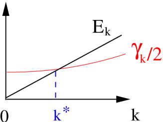
Figure 3: The energy spectrum versus the decay rate of the exciton at a given in-plane momentum $\vec{k}$.

Note that the input-output formalism Eqns.6,9 stands for a non-equilibrium dynamic process. It takes Eqn.5 as the initial state, then solving the coupled Heisenberg equations of the photon and exciton operators. The steady state of the excitons has been reached, the photons are scattering from such an exciton steady state, so the Eqn.6 can be considered as the scattering $S$ matrix shown in the Fig.1.

In the following sections, we will first use the Eqn.6 to calculate the one photon normal and anomalous Green functions, then we will use the Eqn.9 to evaluate all the 5 normal and anomalous exciton correlation functions: the greater $G^{>}$, lesser $G^{<}$, retarded $G^{R}$, advanced $G^{A}$, the time-ordered $G^{T}$ and the Keldysh component $G^{K}$.

III One photon normal and anomalous correlation functions

From Eqn.6, one can compute the photon umber spectrumpower :

$$S_{1}(\vec{k},\omega) = \langle a^{out\dagger}_{\vec{k}}(\omega)a^{out}_{\vec{k}}(\omega)\rangle_{in}=\gamma^{2}_{\vec{k}}|G_{a}(\vec{k},\omega+i\frac{\gamma_{k}}{2})|^{2}$$ (10)

$$= \frac{\gamma^{2}_{\vec{k}}\bar{n}^{2}V_{d}^{2}(\vec{k})}{\Omega^{2}(\omega)+\gamma_{\vec{k}}^{2}E^{2}(\vec{k})}$$

where $\Omega(\omega)=\omega^{2}-E^{2}(\vec{k})+\gamma_{\vec{k}}^{2}/4$.

By using the Fourier transformation to $S_{1}(\vec{k},\omega)$, one can get $G_{\pm}(\vec{k},\tau)=G_{1}(\vec{k},\tau)$

$$G_{1}(\vec{k},\tau)=\frac{\bar{n}^{2}V_{d}^{2}(k)\gamma_{k}}{4E(k)}[\frac{e^{i(E(k)+i\frac{\gamma_{k}}{2})\tau}}{E(k)+i\frac{\gamma_{k}}{2}}+h.c.]$$ (11)

which, obviously, only depends on the anomalous Green function $G_{a}(\vec{k},\omega)$.

The normalized first order correlation function $g_{\pm}(\vec{k},\tau)=g_{1}(\vec{k},\tau)=G_{1}(\vec{k},\tau)/G_{1}(\vec{k},\tau=0)$. When $\tau>0$, it is given by:

$$g_{1}(\vec{k},\tau)=e^{-\frac{\gamma_{\vec{k}}}{2}\tau}[\cos(E(\vec{k})\tau)+\frac{\gamma_{\vec{k}}}{2E(\vec{k})}\sin(E(\vec{k})\tau)]$$ (12)

It turns out that the first order correlation function is independent of the relation between $E(\vec{k})$ and $\gamma_{\vec{k}}/2$.

Similarly, one can find:

$$\langle a^{out}_{\vec{k}}(\omega)a^{out\dagger}_{\vec{k}}(\omega)\rangle=|-1+\gamma_{\vec{k}}G_{n}(\vec{k},\omega+i\frac{\gamma_{k}}{2})|^{2}$$ (13)

which, in sharp contrast to Eqn.11, only depends on the normal Green function $G_{n}(\vec{k},\omega)$.

The power spectrum experiments power only measure the normal ordered one photon correlation function Eqn.11. The anti-normal ordered one photon correlation function Eqn.13 maybe measured by a transmission spectrum with a weak external pumping.

One can also calculate the anomalous one photon Green function:

$$\langle a^{out}_{\vec{k}}(\omega)a^{out}_{-\vec{k}}(-\omega)\rangle = [-1+\gamma_{\vec{k}}G_{n}(\vec{k},\omega+i\frac{\gamma_{k}}{2})]$$ (14)

$$\times \gamma_{\vec{k}}G_{a}(\vec{k},-\omega+i\frac{\gamma_{k}}{2})$$

which depends on both the normal and the anomalous Green functions.

By changing $\vec{k}\rightarrow-\vec{k},\omega\rightarrow-\omega$ in Eqn.14, one can get:

$$\langle a^{out}_{-\vec{k}}(-\omega)a^{out}_{\vec{k}}(\omega)\rangle = [-1+\gamma_{\vec{k}}G_{n}(\vec{k},-\omega+i\frac{\gamma_{k}}{2})]$$ (15)

$$\times \gamma_{\vec{k}}G_{a}(\vec{k},\omega+i\frac{\gamma_{k}}{2})$$

From the explicit forms of $G_{n},G_{a}$ listed in Eqn.7, one can observe that the right hand side of Eqn.14 is a even function of $\omega$, so:

$$\langle a^{out}_{\vec{k}}(\omega)a^{out}_{-\vec{k}}(-\omega)\rangle=\langle a^{out}_{-\vec{k}}(-\omega)a^{out}_{\vec{k}}(\omega)\rangle$$ (16)

This identity is expected because both the input and output fields obey the Bose commutation relations power :

$$[a_{\vec{k}}^{in}(t),a_{\vec{k}^{\prime}}^{in\dagger}(t^{\prime})]=[a_{\vec{k}}^{out}(t),a_{\vec{k}^{\prime}}^{out\dagger}(t^{\prime})]=\delta_{\vec{k},\vec{k}^{\prime}}\delta(t-t^{\prime})$$

$$[a_{\vec{k}}^{in}(t),a_{\vec{k}^{\prime}}^{in}(t^{\prime})]=[a_{\vec{k}}^{out}(t),a_{\vec{k}^{\prime}}^{out}(t^{\prime})]=0$$ (17)

so that $\langle a_{\vec{k}}^{out}(t)a_{-\vec{k}}^{out}(0)\rangle_{in}=\langle a_{-\vec{k}}^{out}(0)a_{\vec{k}}^{out}(t)\rangle_{in}$ whose Fourier transform leads to Eqn.16.

One can also find the Fourier transforms of Eqn.14 and 15:

$$F_{1}(\tau) = \int\frac{d\omega}{2\pi}e^{i\omega\tau}\langle a^{out}_{-\vec{k}}(-\omega)a^{out}_{\vec{k}}(\omega)\rangle$$

$$F_{2}(\tau) = \int\frac{d\omega}{2\pi}e^{i\omega\tau}\langle a^{out}_{\vec{k}}(\omega)a^{out}_{-\vec{k}}(-\omega)\rangle$$ (18)

Using Eqn.16, one can see that $F_{1}(\tau)=F_{2}(\tau)$. Then the normalized anomalous one photon correlation function in the time domain is given by:

$$f_{1}(\tau) = F_{1}(\tau)/G_{1}(0)=-\frac{E^{2}(\vec{k})+\frac{\gamma_{\vec{k}}^{2}}{4}}{\bar{n}V_{d}(\vec{k})}e^{-\frac{\gamma_{\vec{k}}}{2}\tau}$$ (19)

$$\times [u_{\vec{k}}^{2}\frac{e^{-iE(\vec{k})\tau}}{E(\vec{k})-i\frac{\gamma_{\vec{k}}}{2}}+v_{\vec{k}}^{2}\frac{e^{iE(\vec{k})\tau}}{E(\vec{k})+i\frac{\gamma_{\vec{k}}}{2}}]$$

which was used in calculating the two photon correlation functions in squ .

Measuring these photon anomalous Green functions are through the phase sensitive homodyne measurements discussed in the squ .

IV One exciton normal correlation functions

From Eqn.9, one can compute the normal exciton correlation function:

$$iG^{<}_{n}(\vec{k},\omega) = \langle b^{\dagger}_{\vec{k}}(\omega)b_{\vec{k}}(\omega)\rangle_{in}=\gamma_{\vec{k}}|G_{a}(\vec{k},\omega+i\frac{\gamma_{k}}{2})|^{2}$$ (20)

$$= \frac{\gamma_{\vec{k}}\bar{n}^{2}V_{d}^{2}(\vec{k})}{\Omega^{2}(\omega)+\gamma_{\vec{k}}^{2}E^{2}(\vec{k})}$$

where $\Omega(\omega)=\omega^{2}-E^{2}(\vec{k})+\gamma_{\vec{k}}^{2}/4$. Note that it only depends on the anomalous Green function. Obviously, the normalized first order exciton correlation function

$$g_{1b}(\vec{k},\tau)=G_{1b}(\vec{k},\tau)/G_{1b}(\vec{k},\tau=0)=g_{1}(\vec{k},\tau)$$ (21)

is also given by Eqn.12 and shown in Fig.4.

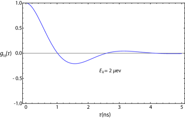
Figure 4: The one exciton correlation function of Eqn.21 at the experimental relevant values diff $nV_{d}(\vec{k})=5\mu eV,\gamma_{\vec{k}}/2=1\mu eV$ at the quasi-particle energies $E(\vec{k})=2\mu eV$. The same values of the $nV_{d}(\vec{k}),\gamma_{\vec{k}}/2$ will also be used draw in Fig.5-10.

From Eqn.9, one can compute the exciton correlation function:

$$iG^{>}_{n}(\vec{k},\omega) = \langle b_{\vec{k}}(\omega)b^{\dagger}_{\vec{k}}(\omega)\rangle_{in}=\gamma_{\vec{k}}|G_{n}(\vec{k},\omega+i\frac{\gamma_{k}}{2})|^{2}$$ (22)

$$= \frac{\gamma_{\vec{k}}[(\omega+\epsilon_{\vec{k}}+\bar{n}V_{d}(\vec{k}))^{2}+(\gamma_{\vec{k}}/2)^{2}]}{\Omega^{2}(\omega)+\gamma_{\vec{k}}^{2}E^{2}(\vec{k})}$$

which only depends on the normal Green function, in sharp contrast to Eqn.20.

From Eqn.22 and Eqn.20, one can find the normal spectral weight

$$\rho_{n}(\vec{k},\omega)=\langle b_{\vec{k}}(\omega)b^{\dagger}_{\vec{k}}(\omega)\rangle_{in}-\langle b^{\dagger}_{\vec{k}}(\omega)b_{\vec{k}}(\omega)\rangle_{in}$$

$$=i[G^{>}_{n}(\vec{k},\omega)-G^{<}_{n}(\vec{k},\omega)]~{}~{}~{}~{}~{}~{}~{}~{}~{}~{}~{}~{}$$

$$=\gamma_{\vec{k}}[|G_{n}(\vec{k},\omega+i\frac{\gamma_{k}}{2})|^{2}-|G_{a}(\vec{k},\omega+i\frac{\gamma_{k}}{2})|^{2}]$$ (23)

Using the Eqn.7, one can manipulates the last equation in 23 into a surprisingly simple result:

$$\rho_{n}(\vec{k},\omega)=i[G_{n}(\vec{k},\omega+i\frac{\gamma_{k}}{2})-G_{n}(\vec{k},\omega-i\frac{\gamma_{k}}{2})]$$ (24)

One can also calculate the Retarded and Advanced normal Green function:

$$iG^{R}_{n}(\vec{k},t) = \theta(t)[b_{\vec{k}}(t),b^{\dagger}_{\vec{k}}(0)]$$

$$iG^{A}_{n}(\vec{k},t) = -\theta(-t)[b_{\vec{k}}(t),b^{\dagger}_{\vec{k}}(0)]$$ (25)

Their Fourier transforms lead to their corresponding normal spectral weight representations:

$$G^{R}_{n}(\vec{k},\omega)=\int\frac{d\omega^{\prime}}{2\pi}\frac{\rho_{n}(\vec{k},\omega^{\prime})}{\omega-\omega^{\prime}+i\eta}$$

$$G^{A}_{n}(\vec{k},\omega)=\int\frac{d\omega^{\prime}}{2\pi}\frac{\rho_{n}(\vec{k},\omega^{\prime})}{\omega-\omega^{\prime}-i\eta}$$ (26)

Plugging the Eqn.24 into the above equations leads to:

$$G^{R}_{n}(\vec{k},\omega)=G_{n}(\vec{k},\omega+i\frac{\gamma_{k}}{2})$$

$$G^{A}_{n}(\vec{k},\omega)=G_{n}(\vec{k},\omega-i\frac{\gamma_{k}}{2})$$ (27)

whose physical pictures are clear: the Retarded or Advanced normal Green functions can be achieved simply by just putting the decay rate $\pm\frac{\gamma_{k}}{2}$ in the non-dissipative ones in Eqn.7.

From Eqns.23,24,27, we can check the identity:

$$G^{R}_{n}-G^{A}_{n}=G^{>}_{n}-G^{<}_{n}$$ (28)

as expected.

We can also compute the Time ordered exciton Green function

$$iG^{T}_{n}(\vec{k},t)=\langle Tb_{\vec{k}}(t)b^{\dagger}_{\vec{k}}(0)\rangle~{}~{}~{}~{}~{}~{}~{}~{}~{}$$

$$=\theta(t)\langle b_{\vec{k}}(t)b^{\dagger}_{\vec{k}}(0)\rangle+\theta(-t)\langle b^{\dagger}_{\vec{k}}(0)b_{\vec{k}}(t)\rangle$$ (29)

Its Fourier transform leads to:

$$G^{T}_{n}(\vec{k},\omega)=\int\frac{d\omega^{\prime}}{2\pi i}[\frac{G^{>}_{n}(\vec{k},\omega^{\prime})}{\omega^{\prime}-\omega-i\eta}-\frac{G^{<}_{n}(\vec{k},\omega^{\prime})}{\omega^{\prime}-\omega+i\eta}]$$ (30)

Substituting Eqn.20, 22 into the above equation and paying special attentions to the pole structures in the Eqn.30, one can show that

$$G^{T}_{n}(\vec{k},\omega) = [1-i\gamma_{\vec{k}}G_{n}(\vec{k},\omega+i\frac{\gamma_{k}}{2})]G_{n}(\vec{k},\omega-i\frac{\gamma_{k}}{2})$$ (31)

$$= [1-i\gamma_{\vec{k}}G^{R}_{n}(\vec{k},\omega)]G^{A}_{n}(\vec{k},\omega)$$

Finally, from Eqn.22 and Eqn.20, we can easily get the Keldysh component of the Green function:

$$iG^{K}_{n}(\vec{k},\omega)=i[G^{>}_{n}(\vec{k},\omega)+G^{<}_{n}(\vec{k},\omega)]~{}~{}~{}~{}~{}~{}~{}~{}~{}~{}~{}~{}$$

$$=\frac{\gamma_{\vec{k}}[(\omega+\epsilon_{\vec{k}}+\bar{n}V_{d}(\vec{k}))^{2}+(\bar{n}V_{d}(\vec{k}))^{2}+(\gamma_{\vec{k}}/2)^{2}]}{\Omega^{2}(\omega)+\gamma_{\vec{k}}^{2}E^{2}(\vec{k})}$$ (32)

which is shown in the Fig.6. It is neither a even nor an odd function.

It is well known that for an equilibrium system, the $G^{>}_{n}$ and $G^{<}_{n}$ are related by the Fluctuation-Dissipation Theorem (FDT) instead of being independent. At $T=0$, the FDT takes the form

$$i[G^{>}_{n}(\vec{k},\omega)+G^{<}_{n}(\vec{k},\omega)]=isgn\omega[G^{>}_{n}(\vec{k},\omega)-G^{<}_{n}(\vec{k},\omega)]$$ (33)

However, for a non-equilibrium system with the initial input state Eqn.5, the $G^{>}_{n}$ in Eqn.22 and the $G^{<}_{n}$ Eqn.20 violate the FDT Eqn.33. Eqn.26 and 30 lead to $G^{R}_{n}$, $G^{A}_{n}$ and $G^{T}_{n}$ respectively. This is an salient feature expected for any non-equilibrium system. The initial input state Eqn.5 is not even an eigen-state, let alone the ground state of the total Hamiltonian Eqn.1. It is this fact which leads to the dynamic photon scattering process encoded in Eqn.6 and 9. The spectral weight $\rho_{n}(\vec{k},\omega)$ in Eqn.23 and the Keldysh component $G^{K}_{n}(\vec{k},\omega)$ in Eqn.32 automatically follow. Detailed comparisons with the corresponding equilibrium system will be given in Sect.IX and the conclusion section.

V One exciton anomalous correlation functions

From Eqn.9, one can also compute the abnormal exciton correlation function $iG^{>}_{a}(\vec{k},\omega)=\langle b_{\vec{k}}(\omega)b_{-\vec{k}}(-\omega)\rangle$:

$$iG^{>}_{a}(\vec{k},\omega)=\gamma_{\vec{k}}G_{n}(\vec{k},\omega+i\frac{\gamma_{k}}{2})G_{a}(\vec{k},-\omega+i\frac{\gamma_{k}}{2})$$

$$=-\frac{\gamma_{\vec{k}}(\omega+i\frac{\gamma_{k}}{2}+\epsilon_{\vec{k}}+\bar{n}V_{d}(\vec{k}))\bar{n}V_{d}(\vec{k})}{\Omega^{2}(\omega)+\gamma_{\vec{k}}^{2}E^{2}(\vec{k})}~{}~{}~{}~{}~{}~{}~{}~{}~{}~{}$$ (34)

which depends on both the normal and the anomalous Green function.

By changing $\vec{k}\rightarrow-\vec{k},\omega\rightarrow-\omega$ in Eqn.34, one can get $iG^{<}_{a}(\vec{k},\omega)=\langle b_{-\vec{k}}(-\omega)b_{\vec{k}}(\omega)\rangle_{in}$:

$$iG^{<}_{a}(\vec{k},\omega)=\gamma_{\vec{k}}G_{n}(\vec{k},-\omega+i\frac{\gamma_{k}}{2})G_{a}(\vec{k},\omega+i\frac{\gamma_{k}}{2})$$ (35)

From Eqn.34 and 35, one find the abnormal spectral weight

$$\rho_{a}(\vec{k},\omega)=i[G^{>}_{a}(\vec{k},\omega)-G^{<}_{a}(\vec{k},\omega)]$$ (36)

When using Eqn.14, 15 and 16, one can manipulate it into a surprisingly simple result:

$$\rho_{a}(\vec{k},\omega)=i[G^{>}_{a}(\vec{k},\omega)-G^{<}_{a}(\vec{k},\omega)]~{}~{}~{}~{}$$

$$=i[G_{a}(\vec{k},\omega+i\frac{\gamma_{k}}{2})-G_{a}(\vec{k},\omega-i\frac{\gamma_{k}}{2})]$$ (37)

In contrast to Eqn.16 for photons, $G^{>}_{a}(\vec{k},\omega)\neq G^{<}_{a}(\vec{k},\omega)$, so $\rho_{a}(\vec{k},\omega)\neq 0$. This is expected, because $\langle b_{\vec{k}}(t)b_{-\vec{k}}(0)\rangle\neq\langle b_{-\vec{k}}(0)b_{\vec{k}}(t)\rangle$.

One can also find the Fourier transforms of Eqn.35 and 34:

$$F_{1b}(\tau) = \int\frac{d\omega}{2\pi}e^{i\omega\tau}iG^{<}_{a}(\vec{k},\omega)$$

$$F_{2b}(\tau) = \int\frac{d\omega}{2\pi}e^{i\omega\tau}iG^{>}_{a}(\vec{k},\omega)$$ (38)

In contrast to the corresponding quantities for photons $F_{1}(\tau)=F_{2}(\tau)$ listed in Eqn.18, $F_{1b}(\tau)\neq F_{2b}(\tau)$. In fact, one can see that $F_{1b}(\tau)=F_{1}(\tau)/\gamma_{\vec{k}},F_{2b}(\tau)=F_{1b}(\tau)-i\bar{n}V_{d}(k)e^{-\frac{\gamma_{\vec{k}}}{2}\tau}\frac{\sin(E(\vec{k})\tau)}{E(\vec{k})}$.

Then the normalized anomalous one exciton correlation function in the time domain is given by:

$$f_{1b}(\tau) = F_{1b}(\tau)/G_{1b}(0)=f_{1}(\tau)$$

$$f_{2b}(\tau) = F_{2b}(\tau)/G_{1b}(0)=f_{1b}(\tau)-i2\frac{E^{2}(\vec{k})+\frac{\gamma_{\vec{k}}^{2}}{4}}{\bar{n}V_{d}(\vec{k})}$$ (39)

$$\times e^{-\frac{\gamma_{\vec{k}}}{2}\tau}\frac{\sin(E(\vec{k})\tau)}{E(\vec{k})}$$

which will be useful in calculating two exciton correlation functions in the Sect.VIII.

One can also calculate the Retarded and Advanced abnormal Green function:

$$iG^{R}_{a}(\vec{k},t) = \theta(t)[b_{\vec{k}}(t),b_{-\vec{k}}(0)]$$

$$iG^{A}_{a}(\vec{k},t) = -\theta(-t)[b_{\vec{k}}(t),b_{-\vec{k}}(0)]$$ (40)

Their Fourier transforms lead to their corresponding spectral weight representations:

$$G^{R}_{a}(\vec{k},\omega)=\int\frac{d\omega^{\prime}}{2\pi}\frac{\rho_{a}(\vec{k},\omega^{\prime})}{\omega-\omega^{\prime}+i\eta}$$

$$G^{A}_{a}(\vec{k},\omega)=\int\frac{d\omega^{\prime}}{2\pi}\frac{\rho_{a}(\vec{k},\omega^{\prime})}{\omega-\omega^{\prime}-i\eta}$$ (41)

Plugging the Eqn.37 into the above equation leads to:

$$G^{R}_{a}(\vec{k},\omega)=G_{a}(\vec{k},\omega+i\frac{\gamma_{k}}{2})$$

$$G^{A}_{a}(\vec{k},\omega)=G_{a}(\vec{k},\omega-i\frac{\gamma_{k}}{2})$$ (42)

whose physical pictures are clear: the Retarded or Advanced anomalous Green functions can be achieved simply by just putting the decay rate $\pm\frac{\gamma_{k}}{2}$ in the non-dissipative ones in Eqn.7.

From Eqns.37, we can check the identity:

$$G^{R}_{a}-G^{A}_{a}=G^{>}_{a}-G^{<}_{a}$$ (43)

as expected.

We can compute the Time ordered anomalous exciton Green function:

$$iG^{T}_{a}(\vec{k},t)=\langle Tb_{\vec{k}}(t)b_{-\vec{k}}(0)\rangle~{}~{}~{}~{}~{}~{}~{}~{}~{}$$

$$=\theta(t)\langle b_{\vec{k}}(t)b_{-\vec{k}}(0)\rangle+\theta(-t)\langle b_{-\vec{k}}(0)b_{\vec{k}}(t)\rangle$$ (44)

Its Fourier transform lead to:

$$G^{T}_{a}(\vec{k},\omega)=\int\frac{d\omega^{\prime}}{2\pi i}[\frac{G^{>}_{a}(\vec{k},\omega^{\prime})}{\omega^{\prime}-\omega-i\eta}-\frac{G^{<}_{a}(\vec{k},\omega^{\prime})}{\omega^{\prime}-\omega+i\eta}]$$ (45)

Substituting Eqn.34,35 into the above equation and paying special attentions to the pole structures in the Eqn.45, one can show that

$$G^{T}_{a}(\vec{k},\omega) = [1-i\gamma_{\vec{k}}G_{n}(\vec{k},\omega+i\frac{\gamma_{k}}{2})]G_{a}(\vec{k},\omega-i\frac{\gamma_{k}}{2})$$ (46)

$$= G^{A}_{a}(\vec{k},\omega)+G^{>}_{a}(\vec{k},\omega)$$

$$= G^{R}_{a}(\vec{k},\omega)+G^{<}_{a}(\vec{k},\omega)$$

Finally, from Eqn.22 and Eqn.20, we can easily get the Keldysh component of the anomalous Green function:

$$iG^{K}_{a}(\vec{k},\omega)=i[G^{>}_{a}(\vec{k},\omega)+G^{<}_{a}(\vec{k},\omega)]$$

$$=-\frac{2\gamma_{\vec{k}}(i\frac{\gamma_{k}}{2}+\epsilon_{\vec{k}}+\bar{n}V_{d}(\vec{k}))\bar{n}V_{d}(\vec{k})}{\Omega^{2}(\omega)+\gamma_{\vec{k}}^{2}E^{2}(\vec{k})}$$ (47)

which is a complex even function. Its real and imaginary part are shown in the Fig.8 and Fig.9 respectively.

Similar to the normal exciton correlation functions discussed in the previous section, as expected for an non-equilibrium system, the $G^{>}_{a}$ in Eqn.34 and $G^{<}_{a}$ Eqn.35 are two independent Green functions, so violates the FDT for anomalous Green function:

$$i[G^{>}_{a}(\vec{k},\omega)+G^{<}_{a}(\vec{k},\omega)]=isgn\omega[G^{>}_{a}(\vec{k},\omega)-G^{<}_{a}(\vec{k},\omega)]$$ (48)

Eqn.41 and 45 lead to $G^{R}_{a}$, $G^{A}_{a}$ and $G^{T}_{a}$ respectively. The spectral weight $\rho_{n}(\vec{k},\omega)$ in Eqn.37 and the Keldysh component $G^{K}_{n}(\vec{k},\omega)$ in Eqn.47 automatically follow. Detailed comparisons with the corresponding equilibrium system will be given in Sect.IX and the conclusion section.

VI Input-output relations between photons and excitons

From the exciton condensation Eqn.3 at $\vec{k}=0$ and the emitted photon number at $\vec{k}=0$ Eqn.4 in Ref.10 ( which is the same as the photon condensation Eqn.62 ), one can immediately see the relation between the two:

$$N_{ph}=N_{b}\gamma_{0}$$ (49)

where the $\gamma_{0}$ is the exciton decay rate at $\vec{k}=0$. This relation relates the condensation of the emitted photon to that of excitons.

From Eqn.10,20, one can see that

$$\langle a^{out\dagger}_{\vec{k}}(\omega)a^{out}_{\vec{k}}(\omega)\rangle_{in}=\gamma_{\vec{k}}\langle b^{\dagger}_{\vec{k}}(\omega)b_{\vec{k}}(\omega)\rangle_{in}$$ (50)

which relates the emitted photon spectrum to the internal normal ordered exciton correlations. A similar relation was discussed in the context of optical cavities book1 ; book2 . Here it is in the spontaneous photon emission from an exciton superfluid in the absence of any cavities. This relation shows that the angle resolved photon power spectrum studied in power can reflect precisely the normal ordered normal exciton correlation function $iG^{>}_{n}$.

However, one can also see that due to the extra first term $1$ in Eqn.13, there is no such simple input-out relation between $\langle a^{out}_{\vec{k}}(\omega)a^{out\dagger}_{\vec{k}}(\omega)\rangle$ and $\langle b_{\vec{k}}(\omega)b^{\dagger}_{\vec{k}}(\omega)\rangle$ listed in Eqn.22.

Now we will try to explore the input-output relation between the anomalous photon correlation function in Eqn.14 and that of the excitons in Eqn.34. Obviously, they are not simply related as the Eqn.50. However, by comparing Eqn.14 with Eqn.46, one can establish the input-output relation between the anomalous photon correlation function with the time-ordered correlation function of the excitons:

$$\langle a^{out}_{\vec{k}}(\omega)a^{out}_{-\vec{k}}(-\omega)\rangle=\gamma_{\vec{k}}iG^{T}_{a}(\vec{k},\omega)$$ (51)

which relates the emitted photon two mode squeezing spectrum to the internal time-ordered exciton correlations. A similar relation was discussed in the context of optical cavities book1 ; book2 . Here it is in the spontaneous photon emission from an exciton superfluid in the absence of any cavities. This relation shows that the phase sensitive homedyne measurements to measure the two mode squeezing spectrum squ can reflect precisely the Time ordered anomalous exciton correlation function $iG^{T}_{a}$. It is instructive to compare Eqn.51 which involves the Time-ordered with Eqn.50 which involves just normal ordered.

VII The quasi-particle spectra and distribution functions in a non-equilibrium stationary exciton superfluid

There are three kinds of Photoluminescence measurements. One kind is the angle resolved power spectrum (ARPS) shown in Fig.3 in power . The second kind is the two mode squeezing spectrum shown in Fig.1b-3a in squ . In any non-equilibrium system, one need both the spectral weight $\rho_{n/a}(\vec{k},\omega)=i[G^{>}_{n/a}(\vec{k},\omega)-G^{<}_{n/a}(\vec{k},\omega)]$ and the Keldysh Green function component $G^{K}_{n/a}(\vec{k},\omega)=G^{>}_{n/a}(\vec{k},\omega)+G^{<}_{n/a}(\vec{k},\omega)$ to characterize the spectral weight and the distribution function respectively. In this section, we will explore the relations between the two kinds of PL with the exciton spectral weights and distribution functions. Due to the lack of FDT in the non-equilibrium exciton superfluid system, these relations are non-trivial, so need to be studied in details. The third kind is the two photon correlations measurement shown in Fig.3b in squ . In the next section, we will explore its relation with the two exciton correlation functions.

VII.1 Connections among the ARPS, the exciton normal spectral weight and distribution function

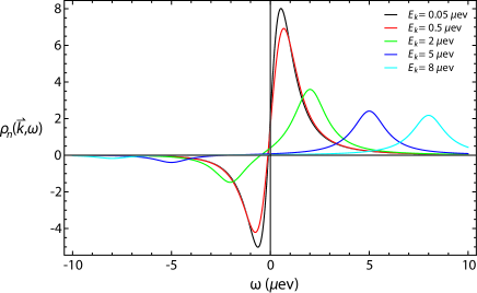
Figure 5: The normal spectral weight Eqn.52 at different quasi-particle energies at $E(\vec{k})<\gamma_{\vec{k}}/2$: $E(\vec{k})=0.05,0.5$ and at $E(\vec{k})>\gamma_{\vec{k}}/2$: $E(\vec{k})=2,5,8\mu eV$.

From Eqn.24, we can get the normal spectral weight $\rho_{n}(\vec{k},\omega)=-2ImG^{R}_{n}(\vec{k},\omega)$:

$$\rho_{n}(\vec{k},\omega) = u^{2}_{\vec{k}}\frac{\gamma_{\vec{k}}}{(\omega-E(\vec{k}))^{2}+(\gamma_{\vec{k}}/2)^{2}}$$ (52)

$$- v^{2}_{\vec{k}}\frac{\gamma_{\vec{k}}}{(\omega+E(\vec{k}))^{2}+(\gamma_{\vec{k}}/2)^{2}}$$

where $u^{2}_{\vec{k}}-v^{2}_{\vec{k}}=1$. Obviously, $\rho_{n}(\vec{k},\omega)$ satisfies the sum rule:

$$\int\frac{d\omega}{2\pi}\rho_{n}(\vec{k},\omega)=u^{2}_{\vec{k}}-v^{2}_{\vec{k}}=1$$ (53)

as expected from its definition.

It is shown in Fig.5 for several different quasi-particle energies $E(\vec{k})$. At $E(\vec{k})=0$, the $\rho_{n}(\vec{k}=0,\omega)=\frac{\gamma_{\vec{k}}}{\omega^{2}+(\gamma_{\vec{k}}/2)^{2}}>0$ is a single Lorentizan centered at $\omega=0$ with width $\gamma_{\vec{k}}/2$. At $E(\vec{k})>0$, it consists of two Lorentizan centered at $\pm E(\vec{k})$ with width $\gamma_{\vec{k}}/2$ with the spectral weight $u^{2}_{\vec{k}}$ and $-v^{2}_{\vec{k}}$ respectively. Only when $E(\vec{k})\gg\gamma_{\vec{k}}/2$ in Fig.5, namely, when $k\gg k^{*}$ in the Fig.3, the two Lorentizans are well separated. Note that $\rho_{n}(\vec{k},\omega=0)=\frac{\gamma_{\vec{k}}}{E^{2}(\vec{k})+(\gamma_{\vec{k}}/2)^{2}}>0$ is large when $E(\vec{k})\leq\gamma_{\vec{k}}/2$. The positive value at $\omega=0$ can be seen in Fig.5 when $E(\vec{k})\leq\gamma_{\vec{k}}/2$. The normal distribution function $iG^{K}_{n}$ is shown in Fig.6.

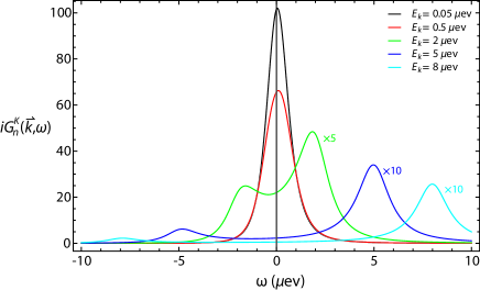
Figure 6: The normal Keldysh component $iG^{K}_{n}$ at different quasi-particle energies $E(\vec{k})=0.05,0.5,2,5,8\mu eV$.

What the first class of PL experiment measured is the angle resolved power spectrum (ARPS) shown in Fig.3 in power . The excitation spectrum and the distribution function of the exciton superfluid system to be probed by transport measurements is given by Eqn.52 and 32 respectively. So it is important to explore the relation between what is measured by the PL and the system’s properties to be probed by transport measurements. Such a relation is given by the input-output relation Eqn.50, Eqn.20 and Eqn.52. One can see qualitatively the same physics with slightly quantitatively different numbers. When $k<k^{*}$, the Fig.5 shows that the quasi-particle is not well defined. Correspondingly, the ARPS in the Fig.3 in power has just one peak pinned at $\omega_{k}=\mu$ with the width $\gamma_{k}$. The MDC has large values at $k<k^{*}$. The EDC has large values at $\omega<\gamma_{k}$. From the Fig.6, one can see that the distribution function has just one peak pinned at $\omega_{k}=\mu$ with the width $\gamma_{k}$. When $k\gg k^{*}$, the Fig.5 shows that the two Lorentizans centered at $\pm E(\vec{k})$ with the width $\gamma_{\vec{k}}/2$ are well separated with two different spectral weights $u^{2}_{\vec{k}}$ and $-v^{2}_{\vec{k}}$ respectively. The quasi-particles at $\pm E(\vec{k})$ are well defined. Correspondingly, the ARPS in the Fig.1 in power has two well defined symmetric quasi-particles peaks at $\omega_{k}=\mu\pm[E^{2}(\vec{k})-\gamma_{\vec{k}}^{2}/4]^{1/2}$ with the width $\gamma_{k}/2$. From the Fig.6, one can see that the distribution function split into two asymmetric peaks at $\omega_{k}=\mu\pm[E^{2}(\vec{k})-\gamma_{\vec{k}}^{2}/4]^{1/2}$ with the width $\gamma_{k}/2$. It is instructive to observe some differences between the $\rho_{n}(\vec{k},\omega)$ shown in the Fig.5 and the ARPS shown in the Fig.3 in power : (1) There are two symmetry peaks in the latter, but the two peaks in the former are as-symmetric with two different spectral weights $u^{2}_{\vec{k}}$ and $-v^{2}_{\vec{k}}$ subject to the constraint $u^{2}_{\vec{k}}-v^{2}_{\vec{k}}=1$. (2) There are very slight differences at the two peak positions, the latter are at $\pm[E^{2}(\vec{k})-\gamma_{\vec{k}}^{2}/4]^{1/2}$, while, the former are at $\pm E(\vec{k})$. The analogies and differences between the $iG^{K}_{n}$ shown in the Fig. 6 and the ARPS shown in the Fig.3 in power can be similarly discussed.

VII.2 Connections among the two mode squeezing spectrum, the exciton abnormal spectral weight and distribution function

Similarly, from Eqn.37, we can get the abnormal spectral weight $\rho_{a}(\vec{k},\omega)=-2ImG^{R}_{a}(\vec{k},\omega)$:

$$\rho_{a}(\vec{k},\omega) = -u_{\vec{k}}v_{\vec{k}}[\frac{\gamma_{\vec{k}}}{(\omega-E(\vec{k}))^{2}+(\gamma_{\vec{k}}/2)^{2}}$$ (54)

$$- \frac{\gamma_{\vec{k}}}{(\omega+E(\vec{k}))^{2}+(\gamma_{\vec{k}}/2)^{2}}]$$

where $u_{\vec{k}}v_{\vec{k}}=\frac{\bar{n}V_{d}(\vec{k})}{2E(\vec{k})}$. It is an odd function of $\omega$ and satisfies the sum rule:

$$\int\frac{d\omega}{2\pi}\rho_{a}(\vec{k},\omega)=0$$ (55)

as expected from its definition.

It is shown in Fig.7 for several different quasi-particle energies $E(\vec{k})$. It also consists of two Lorentizan centered at $\pm E(\vec{k})$ with width $\gamma_{\vec{k}}/2$ with the spectral weights $\mp u_{\vec{k}}v_{\vec{k}}$ respectively. Only when $E(\vec{k})\gg\gamma_{\vec{k}}/2$, namely, when $k\gg k^{*}$ in the Fig.3, the two Lorentizans are well separated. The $\rho_{a}(\vec{k},\omega)$ shown in Fig.7 is an odd function of $\omega$. From Eqn.47, one can see that the anomalous distribution function $iG^{K}_{a}$ is a complex even function, its real and imaginary parts are shown in Fig.8 and Fig.9 respectively. Because the ratio of the real part over the imaginary part is independent of $\omega$, so they have similar shape.

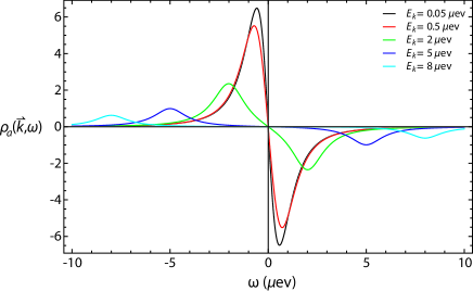
Figure 7: The anomalous spectral weight Eqn.54 at different quasi-particle energies $E(\vec{k})=0.05,0.5,2,5,8\mu eV$.

What the second class of PL experiment measured is two mode squeezing spectrum shown in Fig.1b-3a in squ . The excitation spectrum and distribution function of the exciton superfluid system to be probed by transport measurements are given by Eqn.54 and 47. Such a relation is given by the input-output relation Eqn.51, Eqn.35 and Eqn.54, Eqn.47. One can also see qualitatively the same physics with slightly quantitatively different numbers. When $k<k^{*}$, the Fig.7 shows that the quasi-particle is not well defined. Correspondingly, the two mode squeezing spectrum in the Fig.1b in squ has just one peak centered around $\omega_{k}=\mu$ with the width $\delta_{1}(\vec{k})$ which depends on the dipole-dipole interaction $nV_{d}(\vec{k})$. The corresponding squeezing angle is always positive in all the frequency range as shown in Fig.4a in squ . From the Fig.8 and 9, one can see that the distribution function has just one peak pinned at $\omega_{k}=\mu$ with the width $\gamma_{k}$. When $k\gg k^{*}$, the Fig.7 shows that the two Lorentizans centered at $\pm E(\vec{k})$ with the width $\gamma_{\vec{k}}/2$ are well separated with the spectral weights $\mp u_{\vec{k}}v_{\vec{k}}$ respectively. The quasi-particles at $\pm E(\vec{k})$ are well defined. Correspondingly, the two mode squeezing spectrum in the Fig.3 in squ has two well defined quasi-particles peaks at $\omega_{k}=\mu\pm[E^{2}(\vec{k})-\gamma_{\vec{k}}^{2}/4]^{1/2}$ with the width $\delta_{2}(\vec{k})$ which depends on the dipole-dipole interaction. The corresponding squeezing angle becomes negative at small $|\omega_{k}-\mu|$ and increase to be positive at large $|\omega_{k}-\mu|$, vanishes at the resonant condition $|\omega_{k}-\mu|=[E^{2}(\vec{k})-\gamma_{\vec{k}}^{2}/4]^{1/2}$ as shown in Fig.4a in squ . From the Fig.8 and 9, one can see that the distribution function split into two symmetric peaks at $\omega_{k}=\mu\pm[E^{2}(\vec{k})-\gamma_{\vec{k}}^{2}/4]^{1/2}$ with the width $\gamma_{k}/2$. It is instructive to observe some differences between the Fig.7 and the Fig.1b-3a in squ : (1) The widths in the former also depends on the the dipole-dipole interaction $nV_{d}(\vec{k})$. While the width in the former is just $\gamma_{k}$. (2) There are very slight differences at the two peak positions, the latter are at $\pm[E^{2}(\vec{k})-\gamma_{\vec{k}}^{2}/4]^{1/2}$ where the squeezing angle also vanishes, while, the former are at $\pm E(\vec{k})$. The analogies and differences between the $iG^{K}_{a}$ shown in the Fig.8 and 9 and the Fig.1b-3a in squ can be similarly discussed.

Recently, the elementary excitation spectrum of exciton-polariton inside a micro-cavity was measured expolmode and was found to be very similar to that in a ${}^{4}He$ superfluid except in a small regime near $k=0$. We believe this observation on the anomaly near $k=0$ is precisely due to the excitation spectrum in a non-equilibrium stationary superfluid shown in Fig.5 and Fig.7.

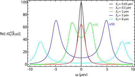
Figure 8: The real part of the anomalous Keldysh component $iG^{K}_{a}$ at different quasi-particle energies $E(\vec{k})=0.05,0.5,2,5,8\mu eV$.

Figure 9: The imaginary part of the anomalous Keldysh component $iG^{K}_{a}$ at different quasi-particle energies $E(\vec{k})=0.05,0.5,2,5,8\mu eV$.

VIII Two exciton correlation functions

In this section, we will explore the relations between the two photon correlations measurements and the two exciton correlation functions. Similar to two photon correlation functions studied in squ , one can also define the two exciton correlations functions:

$$g_{2b}^{(\vec{k})}(\tau) = \frac{\left\langle b_{\vec{k}}^{\dagger}(t)b_{\vec{k}}^{\dagger}(t+\tau)b_{\vec{k}}(t+\tau)b_{\vec{k}}(t)\right\rangle_{in}}{\left|G_{1b}(0)\right|^{2}}$$

$$g_{2b}^{(\pm\vec{k})}(\tau) = \frac{\left\langle b_{\vec{k}}^{\dagger}(t+\tau)b_{\vec{k}}(t+\tau)b_{-\vec{k}}^{\dagger}(t)b_{-\vec{k}}(t)\right\rangle_{in}}{\left|G_{1b}(0)\right|^{2}}$$ (56)

where the $G_{1b}(\tau)=\langle b_{\vec{k}}^{\dagger}(t+\tau)b_{\vec{k}}(t)\rangle_{in}$ is the single exciton correlation function in Eqn.21 and shown in the Fig.4. In order to directly contrast with the two photon correlation functions calculated in squ , we first consider the orderings of the exciton opertaors in Eqn.56. The other orders will be discussed near to the end of this section.

Due to the input-output relation Eqn.50, one can see immediately that $g_{2b}^{(\vec{k})}(\tau)=g_{2}^{(\vec{k})}(\tau)$ which is given in Eqn.12 in squ . However, due to the highly non-trivial input-output relation Eqn.51, the $g_{2b}^{(\pm\vec{k})}(\tau)$ could be even qualitatively differ from $g_{2}^{(\pm\vec{k})}(\tau)$ given in Eqn.12 in squ . This is indeed the case as shown below.

By using Eqn.9 and the commutation relations in the frequency space $[a_{\vec{k}}^{in}(\omega),a_{\vec{k}}^{in\dagger}(\omega^{\prime})]=\delta(\omega-\omega^{\prime})$, one can find

$$G_{2b}^{(\pm\vec{k})}(\tau)=G^{2}_{1b}(\vec{k},\tau=0)+F_{1b}(\tau)\times F^{*}_{2b}(\tau)$$ (57)

where the $F_{1b}(\tau)$ and $F_{2b}(\tau)$ are given in Eqn.39. In fact, one can physically understand Eqn.57 by noting that the first term is due to the equal time single exciton correlation function $G_{1b}(\tau=0)=\langle b_{\pm\vec{k}}^{\dagger}(t)b_{\pm\vec{k}}(t)\rangle$ in the Eqn.21, while the second term is due to the exciton anomalous Green function Eqn.34 which encodes the exciton phase correlations. Because $F_{1b}(\tau)\neq F_{2b}(\tau)$, so the $G_{2b}^{(\vec{k})}(\tau)$ must be complex. Then the normalized two exciton correlation $g_{2b}^{(\pm\vec{k})}(\tau)=1+f_{1b}(\tau)\times f^{*}_{2b}(\tau)$ where the $f_{1b}(\tau)$ and $f_{2b}(\tau)$ are given by Eqn.39, so

$$g_{2b}^{(\pm\vec{k})}(\tau) = g_{2}^{(\pm\vec{k})}(\tau)-i2(\frac{E^{2}(\vec{k})+\frac{\gamma_{\vec{k}}^{2}}{4}}{\bar{n}V_{d}(\vec{k})})^{2}e^{-\gamma_{\vec{k}}\tau}\frac{\sin(E(\vec{k})\tau)}{E(\vec{k})}$$ (58)

$$\times [u_{\vec{k}}^{2}\frac{e^{-iE(\vec{k})\tau}}{E(\vec{k})-i\frac{\gamma_{\vec{k}}}{2}}+v_{\vec{k}}^{2}\frac{e^{iE(\vec{k})\tau}}{E(\vec{k})+i\frac{\gamma_{\vec{k}}}{2}}]$$

The HanburyBrown-Twiss type of experiments are designed to measure the two photon correlation function shown in Fig.3b in squ . The two exciton correlation function of the exciton superfluid system is given by Eqn.58. Although the normalized two photon correlation function $g_{2}^{(\pm\vec{k})}(\tau)$ ( shown in Eqn.12 and Fig.3b in squ ) is always positive, due to the complex second term in Eqn.58, the $g_{2b}^{(\pm\vec{k})}(\tau)$ remains complex. We can separately evaluate both the real part and the imaginary part of the difference of the two:

$$Reg_{2b}^{(\pm\vec{k})}(\tau) - g_{2}^{(\pm\vec{k})}(\tau)=-2\frac{E^{2}(\vec{k})+(\frac{\gamma_{\vec{k}}}{2})^{2}}{(\bar{n}V_{d}(\vec{k}))^{2}}e^{-\gamma_{\vec{k}}\tau}$$

$$\times [\sin^{2}E(\vec{k})\tau-\frac{\gamma_{\vec{k}}}{4E(\vec{k})}\sin 2E(\vec{k})\tau]$$

$$Img_{2b}^{(\pm\vec{k})}(\tau) = -\frac{E^{2}(\vec{k})+(\frac{\gamma_{\vec{k}}}{2})^{2}}{(\bar{n}V_{d}(\vec{k}))^{2}}e^{-\gamma_{\vec{k}}\tau}(u^{2}_{\vec{k}}+v^{2}_{\vec{k}})$$ (59)

$$\times [\sin 2E(\vec{k})\tau+\frac{\gamma_{\vec{k}}}{E(\vec{k})}\sin^{2}E(\vec{k})\tau]$$

which is drawn in the Fig.10.

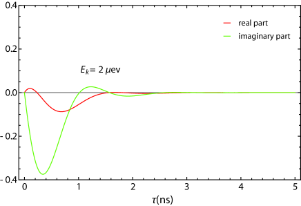
Figure 10: Real and Imaginary part of the two exciton correlation functions Eqn.59 for $E(\vec{k})=2\mu eV$.

When comparing the two exciton correlation function with the single exciton correlation function in Eqn.21 and shown in the Fig.4, one can see that the envelop function in the former ( latter ) decays with the $\gamma_{\vec{k}}$ ( $\gamma_{\vec{k}}/2$ ), the oscillation frequency in the former ( latter ) is $2E(\vec{k})$ ( $E(\vec{k})$ ).

One can see why $g_{2b}^{(\vec{k})}(\tau)$ in Eqn.56 must be positive definite. Define $A^{\dagger}=b_{\vec{k}}^{\dagger}(t)b^{\dagger}_{\vec{k}}(t+\tau),A=b_{\vec{k}}(t+\tau)b_{\vec{k}}(t)$, so the numerator can be written as $H=A^{\dagger}A$ which, of course, is a positive definite Hermitian operator. Similar arguments can be used used to show the two photon correlation functions defined in squ must be positive definite. In fact, one can calculate various two exciton correlation functions by shifting the orders of the exciton operators or put Time-ordered inside the Eqn.56. For example, one can consider $\left\langle b_{\vec{k}}^{\dagger}(t+\tau)b^{\dagger}_{-\vec{k}}(t)b_{-\vec{k}}(t)b_{\vec{k}}(t+\tau)\right\rangle_{in}$, if one define $A^{\dagger}=b_{\vec{k}}^{\dagger}(t+\tau)b^{\dagger}_{-\vec{k}}(t),A=b_{-\vec{k}}(t)b_{\vec{k}}(t+\tau)$, the argument can be written as $H=A^{\dagger}A$, so it must be positive definite. Similar procedures as above lead to its value $1+|f_{1b}(\tau)|^{2}=g_{2}^{(\pm\vec{k})}(\tau)$. One can show that the other two orderings lead to $1+|f_{2b}(\tau)|^{2}$ which is positive definite and $1+f^{*}_{1b}(\tau)\times f_{2b}(\tau)=g_{2b}^{*(\pm\vec{k})}(\tau)$ which is complex conjugate to Eqn.58 and shown in the Fig.10 by adding a minus sign to the imaginary part.

Various exciton correlation functions discussed in this section are needed to evaluate the transport properties of excitons such the Coulomb drag and the counterflow resistances.

IX Exciton correlation functions in an equilibrium dissipative exciton superfluid

In this section, we will study the Exciton correlation functions in an dissipative equilibrium exciton superfluid in Fig.2 and then compare with those in the stationary non-equilibrium exciton superfluid in Fig.1 studied in all the previous sections.

As shown in the Sec.II, in the rotating frame with the frequency $\mu$, the quantum open system in Fig.1 has the Hamiltonian Eqn.2 and the effective quadratic Hamiltonian Eqn.4. In the lab frame, the equilibrium system in Fig.2 have the same Hamiltonian. Staring from Eqn.2 and effective quadratic Hamiltonian Eqn.4, we will discuss $\vec{k}=0$ and $\vec{k}\neq 0$ respectively.

At $\vec{k}=0$, the Hamiltonian for the photons are:

$$H_{0} = \sum_{k_{z}}(v_{g}|k_{z}|-\mu)a^{\dagger}(k_{z})a(k_{z})$$ (60)

$$+ i\sum_{k_{z}}\sqrt{N}(g(k_{z})a-g^{*}(k_{z})a^{\dagger})$$

Obviously, it can be rewritten as

$$H_{0}=\sum_{k_{z}}(v_{g}|k_{z}|-\mu)(a^{\dagger}(k_{z})-\langle a(k_{z})\rangle^{*})(a(k_{z})-\langle a(k_{z})\rangle)+const.$$

$$\langle a(k_{z})\rangle=\frac{ig(k_{z})\sqrt{N}}{v_{g}|k_{z}|-\mu}~{}~{}~{}~{}~{}~{}~{}~{}~{}~{}~{}~{}~{}~{}~{}~{}~{}~{}~{}~{}~{}~{}~{}~{}$$ (61)

where $\langle a(k_{z})\rangle$ is the expectation value of the photon annihilation operator in the ground state. Because the coupling constant $g(k_{z})\sim L^{-1/2}_{z}\rightarrow 0$ in the $L_{z}\rightarrow\infty$ limit, so a proper regulization is needed to extract the physics embedded in this expectation value. This was done in power . Following the regulization procedure in power , we can find the average photon number in the ground state

$$n_{\omega_{k_{z}}}=N\gamma_{0}\delta(v_{g}|k_{z}|-\mu)$$ (62)

where the $\gamma_{0}=|g|^{2}D$ is the exciton decay rate at $\vec{k}=0$ where the $D=L_{z}/v_{g}$ is the photon density of states at $\vec{k}=0$. One can see that the $\gamma_{0}$ is independent of $L_{z}$ and is an experimentally measurable quantity power . The photon condensation Eqn.62 is the same as the emitted photon number at $\vec{k}=0$ Eqn.4 in Ref.10.

Now we will calculate the exciton correlations at $\vec{k}\neq 0$ in the ground state of the interacting system. Obviously, the exact ground state of the interacting systems $|G\rangle$ in Fig.2 is not the same as the initial input state in Eqn.5:

$$|G\rangle\neq|in\rangle=|BEC\rangle|0\rangle_{ph}$$ (63)

Even we do not know the explicit form of $|G\rangle$, we are still able to calculate all the ground state correlation functions by the imaginary time path-integral method which is particularly suitable to calculate correlation functions in an equilibrium system scaling .

In the imaginary time path integral representation of the Hamiltonian Eqn.1

$${\cal L} = \sum_{\vec{k}}\int^{\beta}_{0}d\tau[b^{\dagger}_{\vec{k}}(\tau)\partial_{\tau}b_{\vec{k}}(\tau)+a^{\dagger}_{k}(\tau)\partial_{\tau}a_{k}(\tau)]$$ (64)

$$+ \int^{\beta}_{0}d\tau(H_{sf}+H_{ph}+H_{int})$$

Because the total action Eqn.64 is quadratic, integrating out the photons out exactly leads to the effective action for the excitons only:

$${\cal L}_{ex} = \frac{1}{\beta}\sum_{i\omega_{n}}\sum_{\vec{k}}[b^{\dagger}_{\vec{k}}(i\omega_{n})(-i\omega_{n}+\Sigma(\vec{k},i\omega_{n}))b_{\vec{k}}(i\omega_{n})$$ (65)

$$+ (\epsilon_{\vec{k}}+V_{d}(\vec{k})\bar{n})b_{\vec{k}}^{\dagger}(i\omega_{n})b_{\vec{k}}(i\omega_{n})$$

$$+ (\frac{V_{d}(\vec{k})\bar{n}}{2}b_{\vec{k}}^{\dagger}(i\omega_{n})b_{-\vec{k}}^{\dagger}(-i\omega_{n})+h.c.)]$$

where the $\Sigma(\vec{k},i\omega_{n})$ is the self energy due to the integration of photons:

$$\Sigma(\vec{k},i\omega_{n})=\sum_{k_{z}}\frac{|g(k)|^{2}}{i\omega_{n}-(\omega_{k}-\mu)}$$ (66)

where the sum is over continuous modes of photons at a given in-plane momentum $\vec{k}$.

One can easily find the imaginary time ordered ${\cal T}$ normal and anomalous exciton correlation functions justify :

$${\cal G}^{{\cal T}}_{n}(\vec{k},i\omega_{n}) = \frac{i\omega_{n}-\Sigma(\vec{k},i\omega_{n})+\epsilon_{\vec{k}}+\bar{n}V_{d}(\vec{k})}{(i\omega_{n}-\Sigma(\vec{k},i\omega_{n}))^{2}-E^{2}(\vec{k})}$$

$${\cal G}^{{\cal T}}_{a}(\vec{k},\omega) = \frac{-\bar{n}V_{d}(\vec{k})}{(i\omega_{n}-\Sigma(\vec{k},i\omega_{n}))^{2}-E^{2}(\vec{k})}$$ (67)

where the average is with respect to the exact ground state of the system. Obviously, the initial input state Eqn.5 is not even an eigen-state of the system, let alone the ground state. This is the main difference between the equilibrium correlation functions calculated here and those calculated in the previous sections. It is the goal of this section to contrast some analogies and especially, the crucial differences between this two sets of correlation functions.

After doing the analytic continuation $i\omega_{n}\rightarrow\omega+i\eta$ in Eqn.66 and replacing the sum by an integral over the density of state $\sum_{k_{z}}\rightarrow\int d\omega_{k}D_{\vec{k}}(\omega_{k})$, one can see:

$$\Sigma(\vec{k},\omega+i\eta)=P\int d\omega_{k}\frac{D_{\vec{k}}(\omega_{k})|g(k)|^{2}}{\omega-(\omega_{k}-\mu)}+i\gamma_{k}/2$$ (68)

where the $P$ stands for the principle part of the integral and the exciton decay rate $\gamma_{k}$ is:

$$\gamma_{k} = 2\pi\int d\omega_{k}D_{\vec{k}}(\omega_{k})|g(k)|^{2}\delta(\omega-(\omega_{k}-\mu))$$ (69)

$$\sim 2\pi D_{\vec{k}}(\mu)\left|g_{\vec{k}}(\omega_{k}=\mu)\right|^{2}$$

where we made the Markov approximation used in power ; squ . The real part causes a small energy shift which, in fact, vanishes identically within the Markov approximation in power ; squ . Substituting Eqns.68 and 69 into Eqn.67 leads to:

$${\cal G}^{R}_{n}(\vec{k},\omega) = G_{n}(\vec{k},\omega+i\frac{\gamma_{k}}{2})={\cal G}^{A*}_{n}(\vec{k},\omega)$$

$${\cal G}^{R}_{a}(\vec{k},\omega) = G_{a}(\vec{k},\omega+i\frac{\gamma_{k}}{2})={\cal G}^{A*}_{a}(\vec{k},\omega)$$ (70)

which are identical to Eqn.27 and Eqn.42. At first sight, this result may look surprising. However, one can understand it better by comparing the equilibrium dissipative exciton superfluid in Fig.2 discussed in this section with the non-equilibrium exciton superfluid system in Fig.1 discussed in the previous sections. Both systems are described by the same Hamiltonian Eqn.1 and 4, so should have the same excitation spectrum. This leads to Eqn.70 from a very general physical picture. However, what distinguishes the two systems is the initial conditions. Only the distribution function, namely, the Keldysh component $G^{K}$ depends on the initial conditions. While the retarded and advanced Green functions $G^{R}$ and $G^{A}$ depends only on the Hamiltonian. The distribution function for a bosonic equilibrium system is simply given by the Bose distribution function, while that for an non-equilibrium system is determined by the initial conditions, namely the input state Eqn.5.

The greater and lesser normal Green functions at $T=0$ can also be found from the Fluctuation and Dissipation Theorem (FDT):

$$i{\cal G}^{>}_{n}(\vec{k},\omega) = \theta(\omega)\rho_{n}(\vec{k},\omega)$$

$$i{\cal G}^{<}_{n}(\vec{k},\omega) = -\theta(-\omega)\rho_{n}(\vec{k},\omega)$$ (71)

Obviously, they differ from the corresponding Green functions in the non-equilibrium case Eqn.22,20. Of course, we still have the identity:

$${\cal G}^{R}_{n}-{\cal G}^{A}_{n}={\cal G}^{>}_{n}-{\cal G}^{<}_{n}$$ (72)

The real time-ordered $T$ normal Green function can be found:

$${\cal G}^{T}_{n}(\vec{k},\omega) = {\cal G}^{R}_{n}(\vec{k},\omega)\theta(\omega)+{\cal G}^{A}_{n}(\vec{k},\omega)\theta(-\omega)$$ (73)

$$= G_{n}(\vec{k},\omega+i\frac{\gamma_{k}}{2}sgn\omega)$$

Obviously, it differs from the corresponding Green function in the non-equilibrium case Eqn.30.

From Eqn.71, one can get the Keldysh component Green function:

$$i{\cal G}^{K}_{n}(\vec{k},\omega)=i({\cal G}^{>}_{n}(\vec{k},\omega)+{\cal G}^{<}_{n}(\vec{k},\omega))$$

$$=sgn(\omega)\rho_{n}(\vec{k},\omega)=-2Im{\cal G}^{T}_{n}(\vec{k},\omega)$$ (74)

which is nothing but the FDT Eqn.32 in any equilibrium system. Obviously, it is quite different than $iG^{K}_{n}$ in Eqn.32 for the non-equilibrium system.

Very similar expressions for the greater, the lesser, time ordered anomalous Green functions and the Keldysh component can be written down by changing the subscript $n$ from Eqn. 71 to Eqn.74 to the subscript to $a$. Two exciton correlation functions can be computed using the Wick theorems. Their analogies and differences with those of the excitons in non-equilibrium systems calculated in Sec. VIII can be addressed similarly.

Because the retarded and advanced Green functions are the same as those in the non-equilibrium case, so the normal and anomalous spectral weights are the same as those in the non-equilibrium case listed in Eqn.52, 54 and drawn in the Figs.5 and 7. However, the distribution functions are quite different. For the equilibrium case in the Fig.2, the distribution functions are just multiply Figs.5 and 7 by $sgn(\omega)$. While for the non-equilibrium case in the Fig.1, the distribution functions are shown in the Fig.6,8 and 9.

X Conclusions

In this paper, by using the Heisenberg-Langevin equations in the context of the input-output formalism, we calculated various one and two exciton correlation functions and also explored their relations to various photon correlation functions. We evaluated both the normal and abnormal spectral weights which lead to the excitation spectra of the non-equilibrium exciton superfluids. We also studied both the normal and abnormal Kelydsh component Green functions which lead to the distribution functions of the non-equilibrium exciton superfluids. These relations brought out the important connections between the properties of exciton superfluid systems to be probed by transport easurements and the various quantum optical photoluminescence measurements on emitted photons such as the angle resolved photon power spectrum, phase sensitive homodyne experiments and HanburyBrown-Twiss type of experiments.

By the imaginary time formalism, we calculated the exciton correlations functions of an equilibrium exciton superfluid subject to a photon dissipation bath. It was demonstrated explicitly that $G^{R}_{n/a},G^{A}_{n/a}$ and the spectral weights $\rho_{n/a}$ are the same for the two systems, but the $G^{>}_{n/a},G^{<}_{n/a}$, $G^{T}_{n/a}$ and the distribution functions, namely, the Keldysh component Green functions $G^{K}_{n/a}$ are different. The analogies and differences between the two kinds of systems can be summarized in the Fig.1 and Fig.2. In the equilibrium system in Fig.2, one measures ${\cal G}^{<}$ experimentally which is directly related to the spectral weight $\rho$ by the FDT Eqn.71. ( see also scaling ). The conventional theoretical tool is the imaginary time path integral method which can be analytically continued to the real time as shown in the Sec.IX. While in an non-equilibrium system in Fig.1, in the present context of non-equilibrium exciton superfluids, one also measures $G^{<}_{ph}$ for emitting photons which is related to the corresponding $G^{<}$ for the excitons by the input-output relation Eqn.50 derived in Section VI. Unfortunately, due to the lack of the FDT, the $G^{<}$ for the excitons is not simply related to the spectral weight $\rho$, its relation is non-trivial and need to be studied in details. For the given initial conditions Eqn.5, this relation has been worked out by the Heisenberg equation of motions and was discussed explicitly in Sec.IV-VII. This important feature should hold in any non-equilibrium quantum open system.

The input-output formalism can only be used to study the dynamic scattering process in Fig.1 starting from the input initial state Eqn.5. While the imaginary time path integral method in the section IX can only be used to study the equilibrium case in Fig.2 based on the exact ground state Eqn.63. It was known that the correlation functions in both equilibrium and non-equilibrium quantum open systems could also be calculated by the Keldysh Green function method. The Kelydsh formalism in either Canonical Quantization language or path-integral language can be used to study both the dynamic scattering process in Fig.1 starting from the input initial state Eqn.5 and the the equilibrium case in Fig.2 based on the exact ground state Eqn.63. In a non-equilibrium case, because the $G^{>}_{n/a}$ and $G^{<}_{n/a}$ are independent of each other, one need both the forward and the backward paths in the real-time Keldysh contour. While in an equilibrium case, they are related by Fluctuation and dissipation theorem (FDT), so the forward and backward path can be reduced to just the forward path. In the Kelydsh formalism, one can find $G^{R}_{n/a},G^{A}_{n/a}$, therefore the spectral weight $\rho_{n/a}=i(G^{R}_{n/a}-G^{A}_{n/a})=i(G^{>}_{n/a}-G^{<}_{n/a})$ which leads to excitation spectrum of the interacting system. Most importantly, one can also determine the Keldysh component $G^{K}_{n/a}=G^{>}_{n/a}+G^{<}_{n/a}$ which leads to the distribution function. It is the distribution function which lead to the difference between the equilibrium and the non- equilibrium system. Then one can determine $G^{>}_{n/a}$ and $G^{<}_{n/a}$ respectively and compare with those achieved from the input-output formalism for non-equilibrium system and the imaginary time path integral method for the equilibrium system. Two-exciton correlation functions can also be evaluated by the Keldysh formalism by the counter-ordered Wick theorem. As shown in the Sect.IV-VIII, the procedures using the input-output formalism is just opposite to those using the Kelydsh formalism: one determine $G^{>}_{n/a}$ and $G^{<}_{n/a}$ first, then the spectral weight $\rho_{n/a}=i(G^{>}_{n/a}-G^{<}_{n/a})$, then determine $G^{R}_{n/a},G^{A}_{n/a},G^{T}_{n/a}$ and $G^{K}_{n/a}$. The connections between the Keldysh Green function formalism and the input-output formalism will be explored in details in a future publication sun .

The various one and two exciton correlation functions can be used to calculate the transport properties of the excitons such as the Coulomb drag and counterflow experiments. They are also needed to calculate the superfluid density and the critical velocity of the dissipative superfluids. Indeed, as pointed out in the introduction, the transport properties can provide more direct evidences on superfluids than the spectroscopic properties. The input-output relations can be used to establish the connections between the transport measurements on excitons and the PL measurements. In a future publication, using all the one and two exciton correlation functions derived in this paper, we will compute the Coulomb drags, the counterflow resistances, superfluid densities and critical velocities on both equilibrium dissipative superfluids in the Fig.2 and the non-equilibrium open system in the Fig.1.

As pointed out in the introduction, in this paper, we ignored the spins of the electrons and holes, therefore also the polarization of emitted photons. In fact, the electrons in the conduction band carry spin $s=\pm 1/2$. Due to the spin-orbit coupling, the holes in the valence band carry total spin $J=3/2$. The quantum well confinement potential in the EHBL splits the energy of the light hole with $m_{l}=\pm 1/2$ above that of the heavy hole $m_{h}=\pm 3/2$ spinthe . So we will neglect the higher energy light-hole, only consider the lower energy heavy- hole with $m_{h}=\pm 3/2$. One electron with $s=\pm 1/2$ and one heavy-hole with $m_{h}=\pm 3/2$ can bind into four kinds of heavy-hole excitons $(\pm 1/2,\pm 3/2)$. When coupled to photons, the selection rule of the photon angular momentum is $J=s+m_{h}$, so the 4 kinds of heavy-hole excitons can be grouped into the bight excitons $J=\pm 1$ which couple to the one photon process with the polarization $\sigma=\pm$ and the dark excitons $J=\pm 2$ which do not couple to the one photon process. However, the spins of electrons and holes inside an exciton will relax ( or de-cohere ) due to the spin-orbit couplings in the conduction band and valence band respectively. These individual electron and hole spin flips lead to the conversion from the dark excitons to the bright excitons. The simultaneous flipping of both electrons and holes is due to the Coulomb exchange interaction, it leads to a spin flip between $J=1$ and $J=-1$ inside the bright excitons. In order to make quantitative connection between theoretical predictions with the experiments, it would be important to study how the results achieved in power ; squ and in this paper for spinless excitons will be modified after taking into account of both bright and dark excitons, also the effects of a trap, disorder and finite temperatures.

Acknowledgements

J.Ye thank T. Shi and Longhua Jiang for the collaborations on the previous works power ; squ which are complementary to the present work. J. Ye’s research is supported by NSF-DMR-1161497, NSFC-11074173, NSFC-11174210, Beijing Municipal Commission of Education under grant No.PHR201107121, at KITP is supported in part by the NSF under grant No. PHY11-25915. W.M. Liu’s research was supported by NSFC-10874235.

References

- (1) John M. Blatt, K. W. Böer and Werner Brandt, Phys. Rev. 126, 1691 (1962); L. V. Keldysh and A. N. Kozlov. Sov, Phys. JETP 27, 521-528 (1968).
- (2) W. Kohn and D. Shrrington, Rev. Mod. Phys. 42, 1-11 (1970).
- (3) Yu. E. Lozovik and V. I. Yudson, Pis’ma Zh. Eksp. Teor. Fiz. 22, 556 (1975) [JETP Lett. 22, 274 (1975)].
- (4) L. V. Butov, et al, Nature 417, 47 - 52 (2002); Nature 418, 751 - 754 (2002); C. W. Lai, et al Science 303, 503-506 (2004). D. Snoke, et al Nature 418, 754 - 757, 2002; D. Snoke, Nature 443, 403 - 404 (2006). R. Rapaport, et al, Phys. Rev. Lett. 92, 117405 (2004); Phys. Rev. B 72, 075428 (2005).
- (5) U. Sivan, P. M. Solomon, and H. Shtrikman, Phys. Rev. Lett. 68, 1196 - 1199 (1992). J. A. Seamons, D. R. Tibbetts, J. L. Reno, M. P. Lilly, Appl. Phys. Lett., 90, 052103, (2007). J. A. Seamons, C. P. Morath, J. L. Reno, M. P. Lilly, Phys. Rev. Lett. 102, 026804 (2009). C. P. Morath, John A. Seamons, John L. Reno, Michael P. Lilly, Phys. Rev. B 79, 041305 (2009). C. P. Morath, J. A. Seamons, J. L. Reno, M. P. Lilly, Phys. Rev. B 78, 115318 (2008).
- (6) A.F. Croxall, K. Das Gupta, C.A. Nicoll, M. Thangaraj, H.E. Beere, I. Farrer, D. A. Ritchie, M. Pepper, arXiv:0807.0134v3; A.F. Croxall, K. Das Gupta, C.A. Nicoll, H.E. Beere, I. Farrer, D.A. Ritchie, M. Pepper, arXiv:0812.3319.
- (7) Y. Yamamoto and A. Imamoglu, Mesoscopic quantum optics, John Wiley & Sons, Inc. 1999.
- (8) J. Kasprzak, et.al, Nature 443, 409 - 414 (28 Sep 2006); Hui Deng, et.al, Phys. Rev. Lett. 99, 126403 (2007); Science 4 October 2002 298: 199-202; R. Balili, et.al, Science 18 May 2007 316: 1007-1010; C. W. Lai, et.al, Nature 450, 529 - 532 (22 Nov 2007).
- (9) S. Utsunomiya, et al , Nature Physics 4, 700 - 705 (01 Sep 2008).
- (10) I. B. Spielman et al., Phys. Rev. Lett. 84, 5808 (2000); 87, 036803 (2001); M. Kellogg et al., Phys. Rev. Lett. 88, 126804 (2002); M. Kellogg et al., Phys. Rev. Lett. 93, 036801 (2004).
- (11) For a review, see J. P. Eisenstein and A. H. MacDonald, Nature 432, 9 (2004) and References therein.
- (12) Jinwu Ye and Longhua Jiang, Phys. Rev. Lett. 98, 236802 (2007), Jinwu Ye, Phys. Rev. Lett. 97, 236803 (2006). Jinwu Ye, Annals of Physics, 323 (2008), 580-630.
- (13) J.R. Leonard, et.al, Nano Lett., 2009, 9 (12), 4204-4208, Sen Yang, et.al, Phys. Rev. B 81, 115320 (2010), Phys. Rev. B 81, 115320 (2010).
- (14) Alex A. High, et.al, Science, 321, 229 (2008).
- (15) J. R. Leonard, et.al, arXiv:1203.6239
- (16) Jinwu Ye, T. Shi and Longhua Jiang, Phys. Rev. Lett. 103, 177401 (2009).
- (17) T. Shi, Longhua Jiang and Jinwu Ye, Phys. Rev. B 81, 235402 (2010).
- (18) Jinwu Ye, Jour. of Low Temp. Phys: 158, 882, (2010).
- (19) Giovanni Vignale and A. H. MacDonald, Drag in Paired Electron-Hole Layers, Phys. Rev. Lett. 76, 2786 - 2789 (1996).
- (20) Ben Yu-Kuang Hu, Phys. Rev. Lett. 85, 820 - 823 (2000).
- (21) M. Z. Maialle, E. A. de Andrada e Silva, and L. J. Sham, Exciton spin dynamics in quantum wells, Phys. Rev. B 47, 15776 - 15788 (1993).
- (22) A.L. Fetter and J. D. Walecka, Quantum Theory of Many Particle System, Dover Publications, Inc., 2003.
- (23) See supplementary material at http://link.aps.org/supplemental/ 10.1103/PhysRevLett.103.177401 for the derivation of this input-output relation.
- (24) In order to be consistent with the conventional notations in the Green functions in condensed matter system fetter , compared to the notations used in power ; squ , we made a change .
- (25) In the following, we negelct the on top of the exciton opertaor.
- (26) In order to show clearly the different structures of various correlation functions, we choose different values than those used in power ; squ .
- (27) D. F. Walls and G. J. Milburn, Chapt. 7, Quantum Optics, Springer-Verlag, 1994.
- (28) M. O. Scully and M. S. Zubairy, Quantum Optics, Cambridge University press, 1997.
- (29) When drawing Fig.5-9, for given and various , we use to determine in Eqn.52 in Fig.5, in Eqn.54 in Fig.7 and Eqn.59 in Fig.10.
- (30) For the FDT in an equilibrium quantum spin system see, A. Chubukov, S. Sachdev and Jinwu Ye, Phys.Rev.B, 11919 (1994).
- (31) Here we assume . This is indeed justified under the Markov approximation Eqn.69. the crucial point here is the existence of the large optical characteristic frequency . However, in the dissipative exciton superfluids in BLQH blqhexp ; counterflow ; psdw , there is gapless electron-hole excitations instaed of such a large characteristic frequency, so the Markov approximation never holds in this kind of system. This is also the cruucial differences between the dissipations in quantum optical systems and in condesed matter systems.
- (32) F.D. Sun et.al, in prepararion.