Delay enhanced coherent chaotic oscillations in networks with large disorders

Abstract

We study the effect of coupling delay in a regular network with a ring topology and in a more complex network with an all-to-all (global) topology in the presence of impurities (disorder). We find that the coupling delay is capable of inducing phase coherent chaotic oscillations in both types of networks thereby enhancing the spatiotemporal complexity even in the presence of $50\%$ of symmetric disorders of both fixed and random types. Further, the coupling delay increases the robustness of the networks upto $70\%$ of disorders, thereby preventing the network from acquiring periodic oscillations to foster disorder-induced spatiotemporal order. We also confirm the enhancement of coherent chaotic oscillations using snapshots of the phases and values of the associated Kuramoto order parameter. We also explain a possible mechanism for the phenomenon of delay-induced coherent chaotic oscillations despite the presence of large disorders and discuss its applications.

I Introduction

In recent times, researchers have been interested in studying networks of oscillators with time-delayed coupling because of their wide applications in science Schuster (1989); Niebur (1991); Kozyreff (2000); Wirkus (2002), engineering and technology Heath (2000); Lindsey (1996); Reddy (2000). Considering the fact that in most realistic physical and biological systems Glass et al. (1977); Cooke et al. (1982); Wischert et al. (1994) the interaction signal propagates through media with limited speed, its finite signal propagation time induces a time-delay in the received signal Hu et al. (2001); MacDonald (1989); Swadlow (1985). For example, in biological neural networks, it has been shown that the neural connections are full of variable loops such that the propagation of signal through the loops can result in a large time-delay (synaptic delay), and it is also reported that the axons can generate time-delay upto $300~{}ms$ Swadlow (1985). A typical nonlinear time-delay system is a veritable black box MacDonald (1989) and that the delay coupling itself gives rise to a plethora of novel phenomena, such as delay-induced amplitude death Reddy (2000), phase-flip bifurcation Prasad et al. (2006), synchronizations of different types Dhamala et al. (2004), multistability Shayer et al. (2000), chimera states sethia et al. (2008); Jane et al. (2009), etc. in coupled nonlinear oscillator systems.

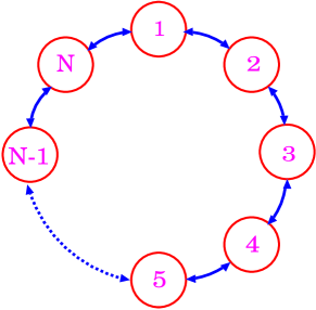
Figure 1: (Colour online) The schematic diagram of the array of pendula with periodic boundary conditions.

In this paper, we consider a network of forced and damped nonlinear pendula studied earlier by Braiman et al.Braiman et al. (1995), commonly known as the forced Frenkal-Kontorova model. It represents a straightforward physical realization of an array of diffusively coupled Josephson junctions Ustinov et al. (1993); Pagano et al. (1986) in which the applied current in each junction is modulated by a common frequency. The possibility of obtaining synchronized motion in one and two-dimensional chaotic arrays of such systems has been investigated in Refs. Weiss et al. (2001, 2001); Zhou et al. (2008); Gavrielides et al. (1998), where the complex chaotic behavior of the collective systems was completely tamed when a certain amount of impurities (disorder) was introduced. To be specific, disorder enhanced spatiotemporal regularity Braiman et al. (1995); Qi et al. (2003), disorder enhanced synchronization Brandt et al. (2006); Braiman et al. (1995) and taming chaos with disorder Weiss et al. (2001, 2001); Gavrielides et al. (1998) in such systems have received central importance in recent research on complex systems and their applications.

In our present studies, we study a regular network with a ring topology and a more complex network with an all-to-all (global) topology with different densities (sizes) of impurities (disorder) and examine the effect of time delay in the coupling. In particular, the oscillations of each pendulum affects the oscillations of the pendula to which it is connected to, after some finite time-delay $\tau$. In such a configuration, we are interested in investigating the possibility of achieving coherent chaotic dynamics in the network despite of the presence of a substantial amount of disorder and, thereby, enhancing the spatiotemporal complexity, a counter-intuitive result to the expected (reported) outcome of taming chaos and enhancing spatiotemporal order with even a negligible size of disorder in the network (in the absence of coupling delay). Here by coherent chaotic dynamics, we mean the emergence of collective (phase-coherent or phase synchronized) chaotic oscillations (but not complete synchronization) in the entire network despite the presence of disorder Brandt et al. (2006). The delay enhanced phase-coherent chaotic oscillations are characterized both qualitatively and quantitatively using snapshots of the phases of the pendula in the networks and the Kuramoto order parameter MacDonald (1989). Recently, similar coherent states have been observed in Bose-Einstein condensates on tilted lattices for strong field showing highly organized patterns, often denoted as quantum carpets Braiman et al. (1995). Enhancing spatiotemporal complexity or at least preserving the original spatiotemporal pattern in the midst of a noisy environment due to the presence of disorder is crucial for applications, such as spatiotemporal and/or secure communication Eurich et al. (2005) in spatially extended systems, especially in biology and physiology Eurich et al. (2005), in the state of art of modern computing, namely liquid state machines (LSM), in which the degree of spatiotemporal complexity of the network of dynamical systems determines the highest degree of computational performance (i.e, mixing property) Eurich et al. (2009), etc.

In particular, we will show that time-delay in the coupling induces coherent chaotic oscillations of the network of coupled systems, in both diffusively coupled pendula with periodic boundary conditions and in a globally coupled network, thereby enhancing the spatiotemporal complexity despite the presence of a large number of disorders, even upto half the size of the network. Further, coupling delay enhances the robustness of the network against disorders of size greater than $50\%$ of the network thereby preserving the original dynamical states of the network and preventing disorder-enhanced synchronous periodic oscillations of the entire network leading to spatiotemporal order. It is to be noted that in an array without delay even the presence of a very small periodic disorder itself is capable of suppressing the chaotic oscillations of the entire network and thereby inducing spatiotemporal regularity as demonstrated in Refs. Weiss et al. (2001, 2001); Gavrielides et al. (1998). We will also explain an appropriate mechanism for delay-induced coherent chaotic oscillations leading to enhanced spatiotemporal complexity based on a mechanism for taming chaoticity (in the absence of delay), as reported in Braiman et al. (1995). A relevant study focusing on macroscopic properties of the globally connected heterogeneous neural network has revealed similar irregular collective behavior Eurich et al. (2009).

The paper is organized as follows. In Sec. II, we will briefly discuss the existing results on taming chaoticity leading to spatiotemporal regularity without any delay coupling for a linear array of nonlinear pendula with periodic boundary conditions, which will be useful for a later comparison. We will demonstrate our results on delay-induced coherent chaotic oscillations despite the presence of large disorders, even upto $70\%$, in Sec. III. Similar results are presented in a network of globally coupled pendula both with and without delay coupling in Sec. IV. Finally, in Sec. V, we discuss our results and conclusions.

II Linear array of pendula in the absence of coupling delay

We consider a chain of $N$ forced coupled nonlinear pendula whose equation of motion can be written as Braiman et al. (1995); Brandt et al. (2006); Weiss et al. (2001, 2001); Gavrielides et al. (1998); Braiman et al. (1995); Qi et al. (2003)

$$ml^{2}\dot{x_{i}} = y_{i},$$ (1a)

$$\dot{y_{i}} = -\gamma y_{i}-mgl~{}sin~{}x_{i}+f+f^{\prime}_{i}sin(\omega t)+$$ (1b)

$$C[y_{i+1}(t)-2y_{i}(t)+y_{i-1}(t)],$$

where $i=1,2,\cdots,N$. We choose the following periodic boundary conditions: $x_{0}=x_{N}$ and $x_{N+1}=x_{1}$. The parameters are taken as follows: the mass of the bob $m=1.0$, the damping $\gamma=0.5$, acceleration due to the gravity $g=1.0$, dc torque $f=0.5$, angular frequency $\omega=0.67$, pendulum length $l=1.0$, $f^{\prime}_{i}=f^{\prime}$ is the ac torque and $C$ is the coupling strength. The schematic diagram of the coupling configuration is shown in Fig. 1, in which the first pendulum is connected with the second and the $N^{th}$ pendulum so that each pendulum gets two inputs, without any delay, from its nearest pendula. For the coupling strength $C=0.0$, the pendula are uncoupled and evolve independently.

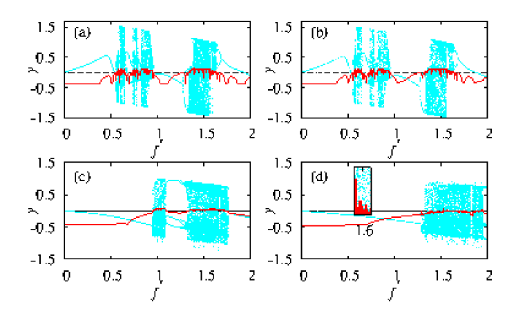
Figure 2: (Color online) Bifurcation diagrams of a single pendulum in a ring of three coupled pendula and the largest Lyapunov exponent (of a single pendulum for $C=0.0$ and that of the entire network for $C>0.0$) for different values of the coupling strength $C$ and the coupling delay $\tau$. (a) $C=0.0$ and $\tau=0.0$, (b) $C=0.5$ and $\tau=0.0$, (c) $C=0.5$ and $\tau=1.5$, and (d) $C=0.6$ and $\tau=2.0$ (inset shows that the pendulum exhibits chaotic oscillations for $f^{\prime}_{d}=1.6$).Red (dark grey) line corresponds to the largest Lyapunov exponent and light blue (light grey) dots correspond to the bifurcation diagram. Note that in all the cases (b)-(d) the three pendula are in a completely synchronized state and, hence, the largest Lyapunov exponent corresponds to the synchronization manifold.

In earlier studies Braiman et al. (1995); Brandt et al. (2006); Weiss et al. (2001, 2001); Gavrielides et al. (1998); Braiman et al. (1995); Qi et al. (2003), the authors have dealt with an array of pendula with diffusive coupling but without delay and have shown that the chaotic dynamics of the array is controlled by the inclusion of impurities, which are disorders in their natural frequencies and/or distributed initial phases of the external forces. In particular, in Ref. Weiss et al. (2001, 2001); Gavrielides et al. (1998), the authors have considered a chain of diffusively coupled pendula without delay and have shown that inclusion of even a single periodic impurity is enough to tame chaos in a long chain of length with $N=512$. However, we would like to point out that we are not able obtain the results with a single impurity as reported by these authors. Nevertheless, taming chaos and achieving spatiotemporal regularity can be obtained for $20\%$ of impurities for appropriate coupling strength for different sizes of the array as reported by other authors Braiman et al. (1995, 1995); Qi et al. (2003); Brandt et al. (2006). In the following, we will briefly illustrate the results of taming chaos and achieving spatiotemporal regularity in an array of $N=50$ coupled pendula, Eq. (1), with ring configuration without any coupling delay to appreciate the effect of delay coupling in the following sections. The results have been confirmed for the case of $N=512$ too.

We introduce disorder in the network of chaotic pendula by allowing one or more pendula to oscillate periodically as in the earlier reports Braiman et al. (1995, 1995); Qi et al. (2003); Brandt et al. (2006). In order to fix the parameters (of the pendula) corresponding to the chaotic and periodic regions, we start our analysis by plotting the bifurcation diagram of a single pendulum as a function of the ac torque in the range $f^{\prime}\in(0,2)$ for fixed values of the other parameters. The bifurcation diagram and its corresponding largest Lyapunov exponent is depicted in Fig. 2(a), which exhibit a typical bifurcation scenario leading to chaotic behavior for appropriate values of the ac torque. To elucidate the dynamical behavior of the ring of $N$ coupled pendula as a function of a parameter, we have explored an array of $N=3$ pendula with periodic boundary conditions in plotting the bifurcation diagram, because each pendulum in an array of arbitrary length $N>2$ is coupled with its nearest neighbors and so each of the pendula effectively gets two inputs from its neighbors. Therefore the basic configuration of $N=3$ pendula is sufficient to explain the bifurcation pattern of $N$ coupled pendula in a ring configuration for same values of the parameters. Indeed, we have confirmed that the bifurcation diagram remains the same irrespective of the value of $N$ for the same set of parameter values as in Fig. 2. The bifurcation diagram of a single pendulum in a ring of $N=3$ coupled pendula and the largest Lyapunov exponent of the entire network for the value of the coupling strength $C=0.5$ in the same range of $f^{\prime}$ is depicted in Fig. 2(b). The bifurcation scenario of each pendulum in a ring of $N=3$ coupled pendula is almost identical to that of a single uncoupled pendulum (Fig. 2(a)) and the network (ring of $N=3$ coupled pendula) as a whole exhibits a positive largest Lyapunov exponent as shown in Fig. 2(b).

It is to be noted that the network of diffusively coupled $(N=3)$ pendula is already in a synchronized state for the chosen value of coupling strength, $C=0.5$. Consequently, following a reasoning similar to what reported in Ref. Boccaletti et al. (2002) for a system of two coupled chaotic oscillators, one gets that the synchronization manifold has only a single positive Lyapunov exponent for appropriate values of $f^{\prime}$. The synchronization manifold in this case is almost similar to the phase space of a single system (Fig. 2(a)) as is evident from the bifurcation diagram (Fig. 2(b)). Hence the network as a whole exhibits a single positive Lyapunov exponent for $C=0.5$. More details on synchronization manifold and its relation to the transition of Lyapunov exponents of diffusively coupled systems can be found in Ref. Boccaletti et al. (2002).

Figure 3: Poincaré points corresponding to the network of pendula in a ring configuration with $N=50$ for the coupling strength $C=0.5$ in the absence of coupling delay. (a) Chaotically oscillating pendula for $f^{\prime}=1.5$ when no disorder is present, (b) Periodically oscillating pendula for $20\%$ disorders with fixed $f^{\prime}=f^{\prime}_{d}=0.5$ and (c) Periodically oscillating pendula for $20\%$ disorders with random $f^{\prime}_{d}\in(0.1,0.5)$.

Figure 4: (Color online) Spatiotemporal representation of Fig. 3. Here the horizontal axis corresponds to time $t$ and the vertical axis to the oscillator index $N$.

Poincaré (surface of section) points corresponding to the network of $N=50$ pendula in a ring configuration, (Eq. (1)), for the coupling strength $C=0.5$ is depicted in Fig. 3. The entire network of pendula exhibits coherent chaotic oscillations in the absence of any periodically oscillating disorder as shown in Fig. 3(a) for the ac torque $f^{\prime}=1.5$. The spatiotemporal representation of Fig. 3(a) is illustrated in Fig. 4(a), where the horizontal axis corresponds to time $t$ and the vertical axis to the oscillator index $N$, which is plotted for ten drive cycles after leaving out sufficient transients (one thousand drive cycles). It is to be noted that the network of $N=50$ coupled pendula does not exhibit synchronous chaotic oscillations as is evident from Fig. 3(a). Otherwise it would show identical color for all the oscillators as a function of time. The colors code the angular velocities of the pendula; dark red (dark gray) indicates negative velocities and green (light gray) positive velocities. Narrow bands of red and green colors represent sudden rapid motion of the pendula in the array. The spatiotemporal plot (Fig. 4(a)) shows that the evolution is not only nonperiodic but is in fact chaotic without any repetitive patterns or regular structures.

Next, impurities (disorders) with periodic oscillations are symmetrically distributed in the array to investigate the effect of disorder as in the earlier studies Braiman et al. (1995); Brandt et al. (2006); Braiman et al. (1995); Qi et al. (2003). It is to be noted that an asymmetric distribution of disorder does not tame the array thereby fostering synchronous evolution and spatiotemporal regularity as discussed in Braiman et al. (1995). The density of the disorder is increased from $1\%$ along with the coupling strength $C$. We find that for $C=0.5$ the entire array gets locked to a synchronous periodic evolution (Fig. 3(b)) for $20\%$ impurities with their corresponding $f^{\prime}_{d}=0.5$ (so that the impurities oscillate periodically), leading to spatiotemporal regularity (Fig. 4(b)). Hereafter, we denote the ac torque corresponding to chaotic states as $f^{\prime}$ and that corresponding to (disordered) periodic states as $f^{\prime}_{d}$. The spatiotemporal plot indicates repetitive patterns for every two drive cycles confirming the periodic evolution of the array of pendula. To be precise, for $20\%$ disorder in the network of $N=50$ coupled pendula, ten disorders are placed at every fifth site in the network. The disorder-induced spatial synchronized states reported here are exactly for the same value of $C$ and the density of the disorders but for different sizes of the array as reported in Refs. Braiman et al. (1995); Brandt et al. (2006); Braiman et al. (1995); Qi et al. (2003). Further, we find that even for a random distribution of $f^{\prime}_{d}$ of the disorders taming can be achieved in a wide range of ac torque. A periodically oscillating array of pendula for $20\%$ of disorder is obtained for a random distribution of $f^{\prime}_{d}\in(0.1,0.5)$ as shown in Fig. 3(c) along with their spatiotemporal representation in Fig. 4(c).

Figure 5: Same as in Fig. 3 but now in the presence of coupling delay $\tau=1.5$ and for different densities of disorders. First row is with fixed value of the disorders $f^{\prime}_{d}=0.5$ and the second row with random values of $f^{\prime}_{d}\in(0.2,0.9)$. (a,d) $20\%$, (b,e) $50\%$ and (c,f) $70\%$ of disorders.

Figure 6: (Color online) Spatiotemporal representation of Fig. 5. Color bar is the same as in Fig. 4.

In the following, we will demonstrate that the introduction of coupling delay can sustain and enhance coherent chaotic oscillations in the linear array with periodic boundary conditions with the density of disorder as large as $50\%$ for the same parameter values. For $50\%$ disorder in the network of $N=50$ coupled pendula, $25$ disorders are placed at every alternate sites in the network. Furthermore, the coupling delay increases the robustness of the network by preserving the dynamical complexity of the given network for further increase in the density of disorder to as large as $70\%$ of the size of the network. The array attains synchronous periodic behavior for disorder greater than $70\%$. For $70\%$ disorders in the network of $N=50$ coupled pendula, after placing $25$ disorders at every alternate sites in the network, the remaining ten disorders are placed anywhere either symmetrically or asymmetrically.

III Linear array with coupling delay

III.1 Effect of Time-delay

Now, we consider a chain of $N$ forced coupled nonlinear pendula with periodic boundary conditions along with the same parameter values as in Sec. II but with the introduction of coupling delay. The dynamical equations then become,

$$ml^{2}\dot{x_{i}} = y_{i},$$ (2a)

$$\dot{y_{i}} = -\gamma y_{i}-mgl~{}sin~{}x_{i}+f+f^{\prime}_{i}sin(\omega t)+$$ (2b)

$$C[y_{i+1}(t-\tau)-2y_{i}(t)+y_{i-1}(t-\tau)],$$

where $i=1,2,\cdots,N$ and $\tau$ is the coupling delay. Now, the first pendulum (see Fig. 1) is connected with the second and with the $N^{th}$ pendulum with a delay $\tau$, so that each pendulum gets two delayed inputs from its nearest pendula. Similar delayed couplings are effective for the other pendula in the array. For $C=0.0$, the pendula are uncoupled and evolve according to their own dynamics as before. As the coupling delay will change the bifurcation scenario of the coupled pendula as a function of the ac torque, we have to look at the bifurcation diagrams to fix the values of the strength of the ac torque $f^{\prime}$ in the periodic and chaotic regimes. The bifurcation scenario of a single pendulum in a ring of $N=3$ delay coupled pendula and the largest Lyapunov exponent of the entire network for the value of the coupling delay $\tau=1.5$ and for $C=0.5$ is depicted in Fig. 2(c). This network exhibits only a single positive Lyapunov exponent for the chosen value of delay $\tau=1.5$, as the network of diffusively coupled subsystems are synchronized to a common synchronization manifold as discussed in Sec. II. Figure 2(d) shows the bifurcation diagram and its corresponding largest Lyapunov exponent for $\tau=2.0$ and $C=0.6$.

The bifurcation diagram (Fig. 2(c)) for $\tau=1.5$ and $C=0.5$ shares some common regimes of chaotic behavior in $f^{\prime}$ with its corresponding undelayed case (Fig. 2(b)). Therefore, we fix $f^{\prime}=1.5$ for the chaotic pendula and $f^{\prime}=f^{\prime}_{d}=0.5$ for disorder characterized by periodic behavior as in Sec. II. The Poincaré points as a function of the oscillator index (N) after leaving out a sufficiently large number of ($1000$ drive cycles) transients in the presence of the coupling delay, $\tau=1.5$, and for $C=0.5$ are shown in Fig. 5 for different values of density of disorder. The first row is plotted for disorders with fixed $f^{\prime}_{d}$ and the second one for a random distribution of $f^{\prime}_{d}\in(0.2,0.9)$. The corresponding spatiotemporal plot is depicted in Fig. 6 for 10 drive cycles. Disorder of size $20\%$ are uniformly distributed in the array of $N=50$ pendula, as in Fig. 3(b) (where the array acquired synchronous periodic oscillations) with fixed and randomly distributed $f^{\prime}_{d}$ in the periodic regime. The evolution of the array in this case is illustrated in Figs. 5(a) and 5(d), respectively. The array self-organizes to exhibit complex spatiotemporal patterns (Figs. 6(a) and 6(d)) without any repetitive patterns thereby exhibiting delay-induced phase-coherent chaotic oscillations (see Sec. III.2 below for confirmation). It is to be noted that the network of $N=50$ delay coupled pendula does not exhibit synchronous oscillations as confirmed by the Figs. 6(a) and 6(d). We have increased the density of disorder upto $50\%$ for the same values of the parameters and the scenario is depicted in Figs. 5(b) and 5(e) for fixed and random distributions of $f^{\prime}_{d}$, respectively, along with the spatiotemporal representation in Figs. 6(b) and 6(e). These figures show that the array of pendula originally with $50\%$ of periodic disorder evolves to acquire collective coherent chaotic oscillations in the entire array induced by the rather small coupling delay $\tau=1.5$ in a wide range of $f^{\prime}$, which is indeed a surprising result of delay impact.

Figure 7: Poincaré points corresponding to the network of pendula, with $f^{\prime}=1.6$ for chaotic pendula, in a ring configuration with $N=50$ for the coupling strength $C=0.6$ with coupling delay $\tau=2.0$ and for different values of density of disorders. First row is with fixed value of the disorders $f^{\prime}_{d}=1.1$ and the second row with random values of $f^{\prime}_{d}\in(0.5,1.2)$. (a,d) $20\%$, (b,e) $50\%$ and (c,f) $70\%$ of disorders.

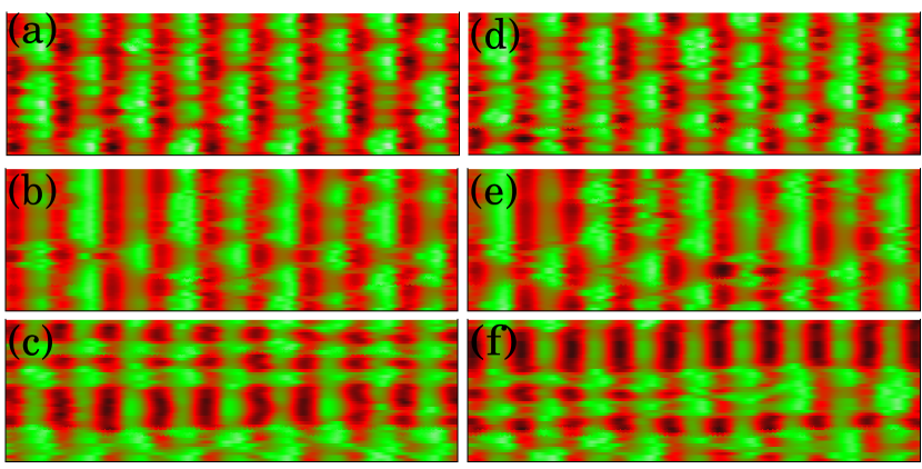
Figure 8: (Color online) Spatiotemporal representation of Fig. 7. Color bar is the same as in Fig. 4.

III.2 Delay enhanced phase coherence

Controlling of oscillator coherence by delayed feedback has been observed both theoretically and experimentally in Refs. Alekseev et al. (2003, 2004). In our investigation, we find that in addtion to the enrichment of the periodic disorder to (chaotic) higher order oscillations, delay coupling also increases the coherence of the collective chaotic oscillations of the whole network. For a better understanding and confirmation of the delay enhanced phase-coherent oscillations of the entire network, we investigate both qualitatively and quantitatively the coherence property of the network macroscopically. For each of the pendulum in system (2), one can define the phase as

$$\theta_{i}=\tan^{-1}(y_{i}/x_{i}).$$ (3)

Here $\theta_{i}$’s represent the phases of the individual pendula in the system. In order to visualize the effect of coupling delay on phase coherence of the system, we plot the snapshot of the phases of the pendula in Fig. 9. From Eq. (3), one can write

$$X_{i} = \cos\theta_{i}=\frac{x_{i}}{\sqrt{(x_{i}^{2}+y_{i}^{2})}},$$ (4a)

$$Y_{i} = \sin\theta_{i}=\frac{y_{i}}{\sqrt{(x_{i}^{2}+y_{i}^{2})}}.$$ (4b)

The Kuramoto order parameter $r$ which quantifies the strength of phase coherence is given by $re^{i\psi}$=$\frac{1}{N}\sum_{j=1}^{N}e^{i\theta_{j}}$. When $r=0$ phase coherence is absent in the system and when $r\approx 1$ there is complete phase coherence in the system. Thus $r$ essentially quantifies the strength of phase coherence. To be more quantitative one can use the time averaged order parameter $R=\frac{1}{T}\int^{T}_{0}rdt$ so that its low value (near to zero) corresponds to phase incoherence while a value near to unity corresponds to phase coherence. Throughout the manuscript, we have estimated $R$ for an average over $1200$ time units.

Figure 9: Snapshots of the phase portraits on the $(X_{i},Y_{i})$ plane of the ring network, with $X_{i}=\cos\theta_{i}$ and $Y_{i}=\sin\theta_{i}$. Here (a) corresponds to $C=0.05$ and (b)-(d) correspond to Figs. 5(d)-(f) with $C=0.5$ and the strength of the impurities being $20\%,50\%$ and $70\%$, respectively.

Using Eqs. (4) (where the $x_{i}$’s are wrapped to be between $0$ and $2\pi$) we have plotted the distribution of phases associated with Eq. (2) in the $(X_{i},Y_{i})$ plane in Fig. 9. We present the results for two specific values of the coupling strength $C$ for the same value of delay parameter $\tau=1.5$, that is for a low value of coupling $C=0.05$ with $20\%$ impurity (Fig. 9(a)) and for $C=0.5$ with $20\%,50\%$ and $70\%$ impurities in Figs. 9(b), (c) and (d), respectively. The phases of the pendula are distributed apart on the unit circle for $C=0.05$, as illustrated in Fig. 9(a), indicating a poor or a very low coherence of the pendula, which is also confirmed by the low value of the time average of the Kuramoto order parameter $R=0.316$. The time evolution of the corresponding order parameter $r$ itself is depicted in Fig. 10(a). The phases of the pendula in the entire network corresponding to Figs. 5(d)-(f), that is for $C=0.5$ with $20\%,50\%$ and $70\%$ impurities, are depicted in Figs. 9(d)-(f), respectively. The phases are now confined to a much smaller region on the unit circle for $C=0.5$ in the presence of the delay coupling confirming the delay enhanced phase-coherent oscillations of the entire network. This is indeed confirmed by much higher values of the time averaged order parameter $R=0.964,0.973$, and $0.982$, for Figs. 9(b)-(d), respectively. Also, the time evolution of the order parameter corresponding to Fig. 9(b) is shown in Fig. 10(b). Thus, we have confirmed the existence of delay enhanced phase-coherent oscillations in the entire network of delay coupled pendula for appropriate coupling strength $C$.

Figure 10: Time evolution of the Kuramoto order parameter $r$ for (a) $C=0.05$ (Fig. 9(a)) and (b) $C=0.5$ with $20\%$ impurity (Fig. 9(b)).

III.3 Possible Mechanism

Two simple mechanism were suggested for taming of chaos by disorder and fostering of periodic patterns in the array without delay in Ref. Braiman et al. (1995). Indeed, we find the manifestations of both these mechanism in the delay coupled networks as well under appropriate conditions. It is essential to understand the first of these two mechanism to understand the mechanism behind the delay induced coherent chaotic oscillations. The first mechanism depends on the topological features of the attractors. The periodic disorder needed to stabilize a chaotic array depends on both the distance and the direction in the parameter space to the nearest periodic attractor, which is controlled by the magnitude and distribution of the disorder Braiman et al. (1995). For this mechanism to work it is not essential to introduce disorder since uncoupled chaotic oscillators can become periodic when coupled. This phenomenon is explicitly observed from the bifurcation diagrams shown in Fig. 2. The chaotic regimes in the range of $f^{\prime}\in(0.5,0.97)$ in Fig. 2(a) for the uncoupled system becomes periodic for the same parameters when a coupling delay is introduced (see Fig. 2(c) and  2(d)). The second mechanism deals with the locking of the chaotic pendula by the periodic ones to the external ac drive Braiman et al. (1995), which is observed for disorder greater than $70\%$ in our case.

Figure 11: (Colour online) Schematic diagram of a network of $5$ oscillators with all to all (global) coupling. In this figure each oscillator gets $4$ delayed input from the remaining oscillators in the network, and also a delayed feedback from itself when $j=i$.

In this paper, we are interested in delay-induced coherent chaotic oscillations in the network, the mechanism of them is a simple extension of the first, as will be explained in the following. The presence of delay in the coupling extends the phase space dimension as a time-delay system is essentially an infinite-dimensional system MacDonald (1989). Therefore, the dimension and the phase space (characterized by multiple unstable directions corresponding to multiple positive Lyapunov exponents of the delay-coupled network) of the chaotic attractors of the delay-coupled network also increases. This in turn increases the robustness of the chaotic attractors against even nearby periodic orbits (disorders) in the parameter space and hence the presence of a large percentage of periodic disorder (which does not extend over multi-dimensional phase space) is not capable of taming the chaoticity of the pendula. Furthermore, delay being a source of instability, by inducing chaotic oscillations Alekseev et al. (1998, 1995, 1995); MacDonald (1989, 1989), the periodic disorder acquires chaotic oscillations for suitable values of the delay resulting in coherent chaotic oscillations of the entire array. It is to be noted that increasing the delay alone gives rise to a rich variety of behavior, such as periodic, higher order oscillations, chaotic and hyperchaotic attractors with a large number of positive Lyapunov exponents as observed in several bifurcation diagrams presented earlier as a function of the delay even in scalar time-delay systems MacDonald (1989); Farmer (1982). Further, periodic orbits of very large periods are also created due to the delay which are not present in the undelayed systems and these higher order oscillation manifest in the array in place of disorder when the size of disorder is larger than $50\%$.

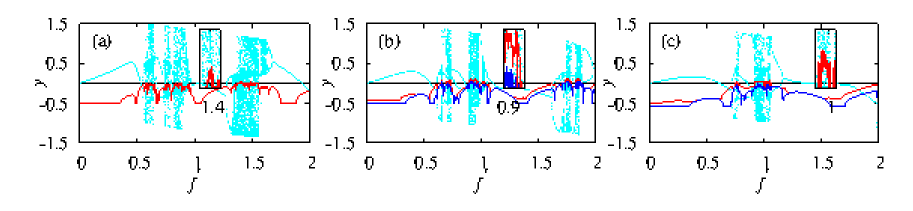
Figure 12: (Color online) The largest Lyapunov exponents of the network of $N=20$ globally coupled pendula and the bifurcation diagram of a single pendulum in the network for different values of the coupling strength $C$ and the coupling delay $\tau$. The inset shows that the network exhibits chaotic oscillations for the specific values of $f^{\prime}$ chosen in the text. (a) $C=0.2$ and $\tau=0.0$, (b) $C=0.2$ and $\tau=1.5$, and (c) $C=0.3$ and $\tau=2.0$. Red and dark blue (dark grey) lines correspond to the largest Lyapunov exponents and light blue (light grey) dots correspond to the bifurcation diagram.

III.4 Effect of Increased Disorder and Coupling Delay

We have also increased the amount of disorder to more than half the size of the network to investigate the effect of delay coupling. Indeed this scenario may also be considered as the one in which chaotic impurities coexist in a sea of a periodically oscillating network and one may expect the suppression of chaotic oscillations to achieve coherent periodic oscillations so as to enhance spatiotemporal order of the network. Nevertheless, the presence of delay in the coupling prohibits suppression of any chaotic pendula upto $70\%$ of disorder and induces chaoticity in the periodic impurities adjacent to a chaotic pendulum, while the impurities away from it acquire higher order oscillations. Furthermore, it is to be noted that for a density of disorder larger than $50\%$, the distribution of disorder becomes nonuniform (asymmetric). For instance, we have distributed $70\%$ of disorders, while retaining chaoticity only in the remaining $30\%$ pendula for the same values of $\tau$ and $C$. The dynamical organization of the array with $70\%$ of disorder is shown in Figs. 5(c) and 5(f), which again depicts the delay-induced chaoticity in the periodic pendula adjacent to the chaotic pendulum, while the other periodic pendula away from the chaotic pendulum acquire higher order oscillations. The corresponding self-organized complex spatiotemporal behavior is shown in Figs. 6(c) and 6(f). We have also confirmed the higher order oscillations of the pendula from their corresponding phase space plots. We can conclude that the complexity of the network as a whole is increased in the presence of delay coupling even if the impurities exceed half the size of the network thereby confirming the robustness of the network against large disorder-induced by the coupling delay.

Next, the value of the coupling delay is further increased to examine whether the delay enhances the coherent chaotic oscillations and increases the robustness of the array against more than $70\%$ disorder. We find that increase in the coupling delay also leads to the same results for appropriate value of the coupling strength and the network of pendula attains synchronous periodic oscillations leading to spatiotemporal order for disorder of size more than $70\%$. To be specific, we fix the coupling delay as $\tau=2.0$ and $C=0.6$. For impurities of periodic type the ac torque is fixed as $f^{\prime}_{d}=1.1$ and for chaotic pendula it is chosen as $f^{\prime}=1.6$ using the bifurcation diagram shown in Fig. 2(d) (as seen in the inset). The first row in Fig. 7 is plotted for disorders with fixed $f^{\prime}_{d}$ and the second row for random distribution of $f^{\prime}_{d}\in(0.2,0.9)$. Delay-induced coherent chaotic oscillations of the whole network in the presence of $20\%$ disorder are shown in Figs. 7(a) and 7(d). The corresponding spatiotemporal representation is illustrated in Figs. 8(a) and 8(d). The network of $N=50$ coupled pendula oscillates chaotically even in the presence of $50\%$ disorder as depicted in Figs. 7(b) and 7(e) along with their complex spatiotemporal patterns in Figs. 8(b) and 8(e), respectively. Further increase in the density of disorder to $70\%$ continues to result in chaotic oscillations of disorders adjacent to the chaotic pendula and higher order oscillations in disorders further away from it, as shown in Figs. 7(c) and 7(f). The corresponding dynamical organization of the network of pendula with $70\%$ disorder to self-organized complex spatiotemporal structures is illustrated in Figs. 8(c) and 8(f).

III.5 Summmary

Thus we have shown that the infected sites are healed or in other words the disorders in the ring network acquires coherent chaotic oscillating behavior induced by time-delay in the coupling thereby enhancing the spatiotemporal complexity for a uniform (symmetric) distribution of the impurities as large as $50\%$ of the array. Note that in the absence of delay in the coupling, the whole network will become infected (ordered) even for $20\%$ of disorder. Further for the density of disorder larger than $50\%$, the distribution of disorder becomes nonuniform (asymmetric). In this case, the impurities adjacent to the chaotic element acquires chaoticity, while the impurities located away from the chaotic ones acquire higher order oscillations resulting in enhanced complexity of the network. It is also to be appreciated that the delay in the coupling not only enhances the coherent chaotic oscillations, but also increases the robustness of the network against any infection (disorder) of even more than half the size of the network.

In the next section, we will extend our investigation to a network of globally coupled pendula and show that we essentially obtain similar results. In particular, coupling delay can enhance the dynamical complexity of disordered pendula leading to delay-induced coherent chaotic oscillations upto $50\%$ of symmetric disorder. For asymmetric disorder of size greater than $50\%$, the coupling delay can induce chaotic oscillations in disordered pendula adjacent to chaotic pendula and those away from it will acquire higher order oscillations upto $65\%$ disorder resulting in the enhanced complex behavior of the existing network.

IV Global delayed coupling

Most natural systems involve complicated coupling between them and that the individual oscillators are not only coupled with their nearest neighbors but also with all other elements in the network. Such a global coupling plays an important role in a large number of dynamical systems ranging from the physical Alekseev et al. (1998), chemical Middya et al. (1994) and biological Winfree (1980) to social and economic Gonzalez et al. (2006); Matassini et al. (2001) networks and electronic systems Visarath et al. (2003). Global coupling is also being studied in reaction-diffusion systems, for example as a reaction-diffusion with global coupling (RDGC) model, to understand the mechanism behind the electromechanic dynamics of the heart and generation of successive ectopic beats Alvarez et al. (2009) and also to understand the mechanism behind the oscillatory regime in the Nash-Panfilov model Nash et al. (2004). In addition, delayed global coupling has been shown to induce in-phase synchronization in an array of semiconductor lasers Kozyreff (2000). It has been demonstrated that global coupling is more efficient than local coupling to achieve non-stationary and stationary in-phase operations with and without delay, respectively, in Ref.Li (1993); Garcia et al. (1999).

In this section, we will investigate the effect of delay coupling in the presence of disorder in a globally coupled network of pendula, where every pendulum is connected to all the other ($N-1$) pendula in the network with a delay $\tau$ and it gets a self-delayed feedback only when $j=i$. To explain the coupling configuration, a schematic diagram of a network of $5$ oscillators is shown in Fig. 11 (the doted lines show the self-delayed feedback only when $j=i$). The model is represented as

$$ml^{2}\dot{x_{i}} = y_{i},$$ (5a)

$$\dot{y_{i}} = -\gamma y_{i}-mgl~{}sin~{}x_{i}+f+f^{\prime}_{i}sin(\omega t)+$$ (5b)

$$\frac{C}{N}\sum_{j=1}^{N}[y_{j}(t-\tau)-y_{i}(t)],$$

where $i=1,2,\cdots,N$. All the parameters have been chosen to be the same as in the previous section. We restrict ourselves to $N=20$ oscillators for computational convenience; however similar results have also been obtained for larger number of oscillators for appropriate coupling delay and coupling strength.

Further, we wish to add that in order to fix the system parameters pertaining to chaotic and periodic regimes, unlike the case of linear coupling (Sec. II and III), it is not meaningful to consider the bifurcation scenario with low numbers of pendula, like $N=3$ or $4$, in the case of global coupling as the bifurcation diagrams will change appreciably when the value of $N$ changes. So in our following study of the bifurcation scenario and the Lyapunov spectrum, we analyse the full network itself and present the first one or two largest Lyapunov exponents of the entire network and the bifurcation diagram of a single pendulum in the network.

Figure 13: Poincaré points of globally coupled network of $N=20$ pendula for the coupling strength $C=0.2$ in the absence of coupling delay $\tau=0.0$. (a) Chaotically oscillating pendula for $f^{\prime}=1.4$, (b) Periodically oscillating pendula for $20\%$ of disorders with fixed $f^{\prime}_{d}=0.3$, and (c) Periodically oscillating pendula for $20\%$ of disorders with random $f^{\prime}_{d}\in(0,0.3)$.

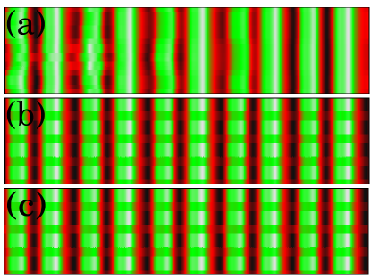
Figure 14: (Color online) Spatiotemporal representation of Fig. 13. Color bar is the same as in Fig. 4.

Figure 15: Poincaré points of globally coupled network of $N=20$ pendula, chaotic for $f^{\prime}=0.92$, for the coupling strength $C=0.2$ and the coupling delay $\tau=1.5$. First row with fixed value of the disorders $f^{\prime}_{d}=1.5$ and the second row with random values of $f^{\prime}_{d}\in(1.0,1.7)$. (a,d) $20\%$, (b,e) $50\%$ and (c,f) $65\%$ of disorders.

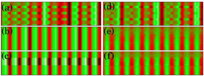
Figure 16: (Color online) Spatiotemporal representation of Fig. 15. Color bar is the same as in Fig. 4.

IV.1 Globally coupled pendula without delay

We will start our investigation by plotting the bifurcation diagrams and the Lyapunov exponents for delineating the periodic and chaotic regimes in the case of $N=20$ globally coupled pendula. Enhancement of spatiotemporal regularity and taming chaoticity in globally coupled network has not yet been reported to the best of our knowledge. Hence the comparison of delay-enhanced coherent chaotic oscillations leading to spatiotemporal complexity will be meaningful only when the globally coupled chaotic network in the presence of a few periodic disorder is tamed when there is no delay. Therefore, in this section, we will show that the globally coupled chaotic network is indeed tamed leading to spatiotemporal order in the absence of coupling delay.

Figure 17: Poincaré points of globally coupled network of $N=20$ pendula, chaotic for $f^{\prime}=0.96$, for the coupling strength $C=0.3$ and the coupling delay $\tau=2.0$. First row with fixed value of the disorders $f^{\prime}_{d}=1.5$ and the second row with random values of $f^{\prime}_{d}\in(1.2,2.0)$. (a,d) $20\%$, (b,e) $50\%$ and (c,f) $65\%$ of disorders.

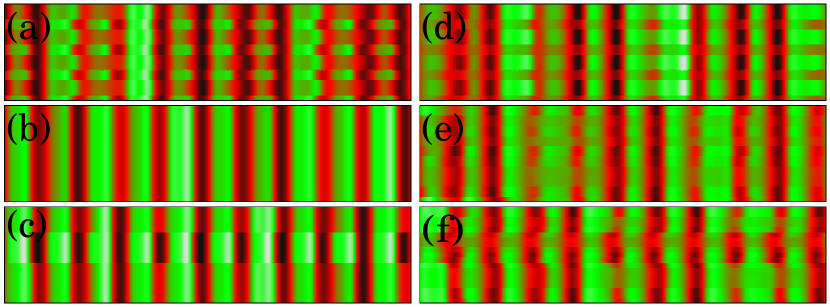
Figure 18: (Color online) Spatiotemporal representation of Fig. 17. Color bar is the same as in Fig. 4.

The largest Lyapunov exponent of the full network and the bifurcation diagram of a pendulum in the network of the globally coupled ($N=20$) case are plotted in Fig. 12(a) for $C=0.2$ in the range of $f^{\prime}\in(0,2)$ when no delay is present. We find that all the pendula in this network exhibit an almost similar bifurcation scenario, and that the network as a whole exhibits multiple positive Lyapunov exponents. However, these values are close to each other and so we present only the largest one in Fig. 12(a). We fix $f^{\prime}=1.4$ for chaotic pendula (as confirmed from the positive Lyapunov exponent shown in the inset of Fig. 12(a)) and $f^{\prime}_{d}=0.3$ for periodic disorder from the bifurcation diagram. Chaotically oscillating pendula in the globally coupled network without any disorder is depicted in Fig. 13(a) for $C=0.2$ along with its spatiotemporal representation in Fig. 14(a) for $10$ drive cycles. As discussed in the case of diffusive coupling in Sec. II, the globally coupled network is also tamed exhibiting periodic oscillations for $20\%$ periodic uniform disorder with fixed $f^{\prime}_{d}=0.3$, as illustrated in Fig. 13(b) for the same value of $C$ in the absence of delay. The corresponding spatiotemporal plot shows spatiotemporal regularity with repetitive patterns for every two drive cycles as depicted in Fig. 14(b). We have obtained similar results of taming chaoticity (Fig. 13(c)) from the network leading to spatiotemporal order (Fig. 14(c)) for random values of the ac torque $f^{\prime}_{d}\in(0,0.3)$. It is also to be noted that we have also got similar results for random values of $f^{\prime}_{d}\in(1.7,2.0)$.

Figure 19: Snapshots of the phase portraits on the $(X_{i},Y_{i})$ plane for a globally coupled network of pendula. Here (a) corresponds to $C=0.05$, and (b)-(d) corresponds to Figs. 15(d)-(f) with $C=0.2$ and the strength of the impurities being $20\%,50\%$ and $65\%$, respectively.

In the next section, we will demonstrate the existence of delay-induced coherent chaotic oscillations leading to enhanced spatiotemporal complexity of the network for disorder of size as large as $65\%$.

IV.2 Globally coupled pendula with coupling delay

The largest two Lyapunov exponents of the network of globally delay coupled pendula and the bifurcation diagram of a single pendulum in the network are plotted in Fig. 12(b) for the same value of coupling delay and coupling strength as in the non-delay case reported in the previous section (Sec. IV.1) for comparison. Again the system as a whole exhibits $20$ positive Lyapunov exponents and only the first two largest positive Lyapunov exponents differ appreciably from the other almost identical positive Lyapunov exponents. Now, we fix $f^{\prime}=0.92$ for chaotic pendula (as confirmed from the positive Lyapunov exponent shown in the inset of Fig. 12(b)) and $f^{\prime}_{d}=1.5$ for periodic disorder from the bifurcation diagram. Poincaré points representing the delay-induced coherent chaotic oscillations of $N=20$ pendula in the network with $20\%$ symmetric disorder with fixed $f^{\prime}_{d}=1.5$ are illustrated in Fig. 15(a) with its complex spatiotemporal patterns in Fig. 16(a). A random distribution of $f^{\prime}_{d}\in(1.0,1.7)$ corresponding to $20\%$ disorder also results in delay-induced coherent chaotic oscillations (Fig. 15(d)) and enhanced spatiotemporal complexity (Fig. 16(d)). The density of disorder is increased further upto half the size of the network with both fixed $f^{\prime}_{d}=1.5$ and random distribution of $f^{\prime}_{d}\in(1.0,1.7)$ as in Figs. 15(b) and  15(e), respectively, which shows increased complexity of the entire network as depicted in their corresponding spatiotemporal plots Figs. 16(b) and  16(e). The globally delay-coupled network remains robust against disorder of a size as large as $65\%$, as shown in Figs. 15(c) and  15(f) for both fixed and random values of ac torque, in which case the period-1 disorder acquires higher order oscillations resulting in a self-organized complex spatiotemporal representation (Figs. 16(c) and  16(f)). For some distributions of $f^{\prime}_{d}$, the network remains robust even upto $70\%$ of disorder.

Figure 20: Time evolution of the Kuramoto order parameter $r$ for (a) $C=0.05$ and (b) $C=0.2$ with $20\%$ impurity.

As in the case of the ring network, we further increased the value of delay in the coupling to examine the change in the robustness of the network against disorder and we obtained the same results even for larger values of delay and for appropriate values of coupling strength. For instance, we present our results for $\tau=2.0$ and $C=0.3$ in the following. The two largest Lyapunov exponents of the network of globally coupled pendula and the bifurcation diagram of a pendulum in the network are illustrated in Fig. 12(c). We chose $f^{\prime}=0.96$ for a chaotic pendulum (as confirmed from the positive Lyapunov exponent shown in the inset of Fig. 12(c)) and $f^{\prime}_{d}=1.5$ for disorders from the bifurcation diagram. Poincaré points shown in Figs. 17(a) and  17(d) indicate the chaotically oscillating pendula for $20\%$ uniform disorder for both fixed and random $f^{\prime}_{d}\in(1.2,2.0)$, respectively. Their spatiotemporal representation is depicted in Figs. 18(a) and  18(d). The evolution of the pendula in the network in the presence of $50\%$ disorder for fixed $f^{\prime}_{d}$ is shown in Fig. 17(b) (with its spatiotemporal plot in Fig. 18(b)) and for random $f^{\prime}_{d}\in(1.2,2.0)$ in Fig. 17(e) (with its spatiotemporal plot in Fig. 18(e)). Figures 17(c) and  17(f) exemplify the dynamical nature of the globally coupled network in the presence of $65\%$ disorder with both fixed and random values of ac torque. The corresponding spatiotemporal dynamics is depicted in Figs. 18(c) and  18(f), respectively. The chaotic pendula remain unaltered, while the period-1 disorders acquire higher order oscillations for sizes larger than $50\%$ resulting in increased spatiotemporal complexity of the original network, indicating the robustness of the delay coupled network against disorder-induced synchronous periodic oscillations.

Finally, as discussed in Sec. III.2, we confirm the existence of the delay enhanced phase-coherent oscillations in the globally connected network of pendula by looking at the distribution of phases in the $(X_{i},Y_{i})$ = $\left(\frac{x_{i}}{\sqrt{x_{i}^{2}+y_{i}^{2}}},\frac{y_{i}}{\sqrt{x_{i}^{2}+y_{i}^{2}}}\right)$ plane. This is indeed shown in Fig. 19. For $C=0.05$ (with 20% impurity) the phases are distributed on a large part of the unit circle (Fig. 19(a)) and this reveals a poor coherence of the pendula as confirmed by the low value of the time averaged order parameter $R=0.267$. The evolution of the corresponding order parameter is depicted in Fig. 20(a). On the other hand, for $C=0.20$ with $20\%,50\%$ and $65\%$ impurities the phases are confined to a narrow region of the unit circle as shown in Figs. 19(b)-(d), which is also confirmed by the corresponding time averaged order parameters $R=0.986,0.988$ and $0.992$, respectively. Also, the evolution of the order parameter $r$ corresponding to Fig. 19(d) is shown in Fig. 20(b).

V Summary and Conclusion

In this paper, we have analyzed the dynamics of a regular network with a ring topology, and a more complex network with all-to-all (global) topology and studied the effect of the size of disorder. We mainly find that the coupling delay can induce phase-coherent chaotic oscillations in the entire network thereby enhancing the spatiotemporal complexity even in the presence of large disorder of a size as large as $50\%$ in contrast to the undelayed case, where even a $20\%$ disorder can render the whole network to be periodic and thereby taming chaos. Furthermore, the delay coupling is also capable of increasing the robustness of the network against a large size of the disorder upto $70\%$ of the size of the original network, thereby increasing the dynamical complexity of the network for suitable values of the coupling strength. We have also discussed a mechanism for the delay-induced coherent chaotic oscillations leading to spatiotemporal complexity in the presence of large disorders. We have also confirmed the delay enhanced coherent chaotic oscillations both qualitatively and quantitatively. We note here that the results are also robust against the size of the network and the size of the impurities (disorders) have to be fixed proportional to the size of the network. We expect that one can use the results of our analysis to more realistic complex networks to increase the robustness of the network against any disorder, for example, in examining the cascading failures of complex networks, specifically in power grids and in controlling disease spreading in epidemics, spatiotemporal and secure communication and to increase the robustness and complexity of reservoir computing or liquid state machines.

VI acknowledgments

The work of R. S, and M. L is supported by the Department of Science and Technology (DST), Government of India-Ramanna program, and also by a DST-IRPHA research project. J. H. S is supported by a DST–FAST TRACK Young Scientist research project. M. L. is also supported by a Department of Atomic Energy Raja Ramanna program. D. V. S and J. K acknowledges the support from EU under project No. 240763 PHOCUS(FP7-ICT-2009-C).

References

- Schuster (1989) H. G. Schuster, and P. Wagner, Prog. Theor. Phys. 81, 929 (1989).
- Niebur (1991) E. Niebur, H. G. Schuster, and D. M. Kammen, Phys. Rev. Lett. 67, 2753 (1991).
- Kozyreff (2000) G. Kozyreff, A. G. Vladimirov, and P. Mandel, Phys. Rev. Lett. 85, 3809 (2000).
- Wirkus (2002) S. Wirkus, and R. Rand, Nonlinear Dyn. 30, 205 (2002).
- Heath (2000) T. Heath, K. Wiesenfeld, and R. A. York, Int. J. Bifurcation Choas. Appl. Sci. Eng. 10, 2619 (2000).
- Lindsey (1996) W. C. Lindsey, and J. H. Chen, Euro. Trans. Tele Commun. 7, 25 (1996).
- Reddy (2000) D. V. RamanaReddy, A. Sen, and G. L. Johnston, Phys. Rev. Lett. 85, 3381 (2000).
- Glass et al. (1977) L. Glass, and M. C. Mackey, Science 197, 287 (1977).
- Cooke et al. (1982) K. L. Cooke, and Z. Grossman, J. Math. Anal. App. 86, 592 (1982).
- Wischert et al. (1994) W. Wischert, A. Wunderlin, A. Pelster, M. Olivier and J. Groslambert, Phys. Rev. E. 49, 203 (1994).
- Hu et al. (2001) B. Hu, Z. Liu, and Z. Zheng, Commun. Theor. Phys. 35, 425 (2001).
- Swadlow (1985) H. A. Shadlow, Neurphysiol. 54, 1346 (1985); F. Aboitiz et al., Brain Res. 598, 143 (1992).
- MacDonald (1989) M. Lakshmanan, and D. V. Senthilkumar, Dynamics of Nonlinear Time-delay Systems (Springer, Berlin, 2011).
- MacDonald (1989) K. Gopalsamy, Stability and Oscillations in Delay Differential Equations of Population Dynamics (Kluwer Academic Publishers, Dordrecht, 1992).
- Prasad et al. (2006) A. Prasad, J. Kurths, S. K. Dana, and R. Ramaswamy, Phys. Rev. E. 74, 035204(R) (2006).
- Dhamala et al. (2004) M. Dhamala, V. K. Jirsa, and M. Ding, Phys. Rev. Lett. 92, 074104 (2004); D. Huber, and L. S. Tsimring, Phys. Rev. Lett. 91, 260601 (2003).
- Shayer et al. (2000) L. P. Shayer, and S. A. Campbell, SIAM J. Appl. Math. 61, 673 (2000).
- sethia et al. (2008) G. C. Sethia, A. Sen, and F. M. Atay, Phys. Rev. Lett. 100, 144102 (2008).
- Jane et al. (2009) Jane H. Sheeba, V. K. Chandrasekar, and M. Lakshmanan, Phys. Rev. E. 79, 055203(R) (2009).
- Braiman et al. (1995) Y. Braiman, J .F. Linder, and W. L. Ditto, Nature 378, 465 (1995).
- Pagano et al. (1986) S. Pagano, M. P. Soerensen, R. D. Parmentier, P. L. Christiansen, O. Skovgaard, J. Mygind, N. F. Pedersen, and M. R. Samuelsen, Phys. Rev. B. 33, 174 (1986).
- Ustinov et al. (1993) A. V. Ustinov, M. Cirillo, and B. A. Malomed, Phys. Rev. B 47, 8357 (1993).
- Zhou et al. (2008) J. Zhou, and Z. Liu, Phys. Rev. E 77, 056213 (2008).
- Weiss et al. (2001) M. Weiss, T. Kottos, and T. Geisel, Phys. Rev. E 63, 056211 (2001).
- Weiss et al. (2001) A. Gavrielides, T. Kottos, V. Kovanis, and G. P. Tsironis, Phys. Rev. E 58, 5529 (1998).
- Gavrielides et al. (1998) A. Gavrielides, T. Kottos, V. Kovanis, and G. P. Tsironis, Europhys. Lett. 44, 559 (1998).
- Qi et al. (2003) F. Qi, Z. Hou, and H. Xin, Phys. Lett. A 308, 405 (2003).
- Braiman et al. (1995) Y. Braiman, W. L. Ditto, K. Wiesenfeld, and M. L. Spano, Phys. Lett. A 206, 54 (1995).
- Brandt et al. (2006) S. F. Brandt, B. K. Dellen, and R. Wessel, Phys. Rev. Lett. 96, 034104 (2006).
- Brandt et al. (2006) Networks with both ring and all-to-all topology exhibits phase synchronous oscillations even with large disorders and we termed the delay enhanced collective chaotic oscillations exhibiting phase synchronization as coherent chaotic oscillations.
- MacDonald (1989) Y. Kuramoto, Chemical Oscillations, Waves, and Turbulence (Springer-Verlag, Berlin, 1984).
- Braiman et al. (1995) A. R. Kolovsky, E. A. Gomez, and H. J. Korsch, Phys. Rev. A 81, 025603 (2010).
- Eurich et al. (2005) J. Garcia-Ojalvo, and R. Roy, Phys. Rev. Lett. 86, 5204 (2001).
- Eurich et al. (2005) S. J. Schiff, K. Jerger, D. H. Duong, T. Chang, M. L. Spano, and W. L. Ditto, Nature 370, 615 (1994).
- Eurich et al. (2009) D. Buonomano, and W. Maass, Nature Rev. Neuosc. 10, 113 (2009).
- Eurich et al. (2009) S. Luccioli, and A. Politi, Phys. Rev. Lett 105, 158104 (2010).
- Boccaletti et al. (2002) S. Boccaletti, J. Kurths, G. Osipov, D. L. Valladares, and C. S. Zhou, Phys. Reports 366, 1 (2002).
- Alekseev et al. (1998) P. W. Roesky, S. I. Doumbouya, and F. W. Schneider, J. Phys. Chem. 97, 398 (1993).
- Alekseev et al. (1995) N. Khrustova, G. Veser, A. Mikhailov, and R. Imbihl, Phys. Rev. Lett 75, 3564 (1995).
- Alekseev et al. (1995) J. M. Aguirregabiria, and L. Bel, Phys. Rev. A 36, 3768 (1987).
- Farmer (1982) J. D. Farmer, Physica D 4, 366 (1982).
- Alekseev et al. (2003) D. Goldobin, M. Rosenblum, and A. Pikovsky, Phys. Rev. E 67, 061119 (2003).
- Alekseev et al. (2004) S. Boccaletti, E. Allaria, and R. Meucci, Phys. Rev. E 69, 066211 (2004).
- Alekseev et al. (1998) A. Alekseev, S. Bose, P. Rodin, and E. Scholl, Phys. Rev. E 57, 2640 (1998).
- Middya et al. (1994) U. Middya, and D. Luss, J. Chem. Phys. 100, 6386 (1994).
- Winfree (1980) A. T. Winfree, The Geomentry of Biological Time (Springer, Heidelberg, 1980); P. C. Matthews, and S. H. Strogatz, Phys. Rev. Lett 65, 1701 (1990).
- Gonzalez et al. (2006) J. C. Gonzlez-Avella, V. M. Eguiluz, M. G. Cosenza, K. Klemm, J. L. Herrera, and M. San Miguel, Phys. Rev. E 73, 046119 (2006).
- Matassini et al. (2001) L. Matassini, and F. Franci, Physica A 289, 526 (2001).
- Visarath et al. (2003) Visarath In, A. Kho, J. D. Neff, A. Palacios, P. Longhini, and B. K. Meadows, Phys. Rev. Lett. 91, 244101 (2003).
- Alvarez et al. (2009) E. Alvarez-Lacalle, and B. Echebarria, Phys. Rev. E 79, 031921 (2009).
- Nash et al. (2004) M. P. Nash, and A. V. Panfilov, Prog. Biophys. Mol. Biol. 85, 501 (2004).
- Li (1993) R. Li, and T. Erneux, Opt. Commun. 99, 196 (1993); M. Silber, L. Fabiny, and K. Wiesenfeld, J. OPt. Soc. Am. B 10, 1121 (1993).
- Garcia et al. (1999) J. Garcia-Ojalvo, J. Casademont, M. C. Torrent, and J. M. Sancho, Int. J. Bifurcation Chaos. Appl. Sci. Eng. 9, 2225 (1999).