Baryon chiral perturbation theory

Abstract

We provide a short introduction to the one-nucleon sector of chiral perturbation theory and address the issue of power counting and renormalization. We discuss the infrared regularization and the extended on-mass-shell scheme. Both allow for the inclusion of further degrees of freedom beyond pions and nucleons and the application to higher-loop calculations. As applications we consider the chiral expansion of the nucleon mass to order ${\cal O}(q^{6})$ and the inclusion of vector and axial-vector mesons in the calculation of nucleon form factors. Finally, we address the complex-mass scheme for describing unstable particles in effective field theory.

I Introduction

Effective field theory (EFT) is a powerful tool in the description of the strong interactions. Generally speaking, an EFT is a low-energy approximation to some underlying, more fundamental theory. The EFT is expressed in terms of a suitable set of effective degrees of freedom, dominating the phenomena in the low-energy region (see Table 1). In the context of the strong interactions, the underlying theory is quantum chromodynamics (QCD)—a gauge theory with color SU(3) as the gauge group. The fundamental degrees of freedom of QCD, quarks and gluons, carry non-zero color charge. Under normal conditions they do not appear as free particles. One assumes that any asymptotically observed hadron must be in a color-singlet state, i.e., a physically observable state is invariant under SU(3) color transformations. The strong increase of the running coupling for large distances possibly provides a mechanism for the color confinement. For the low-energy properties of the strong interactions another phenomenon is of vital importance. The masses of the up and down quarks and, to a lesser extent, also of the strange quark are sufficiently small that the dynamics of QCD in the chiral limit, i.e., for massless quarks, is believed to resemble that of the “real” world. Although a rigorous mathematical proof is not yet available, there are good reasons to assume that a dynamical spontaneous symmetry breaking (SSB) emerges from the chiral limit, i.e., the ground state of QCD has a lower symmetry than the QCD Lagrangian. For example, the comparatively small masses of the pseudoscalar octet, the absence of a parity doubling in the low-energy spectrum of hadrons, and a non-vanishing scalar singlet quark condensate are indications for SSB in QCD. According to the Goldstone theorem, a breakdown of the chiral $\mbox{SU(3)}_{L}\times\mbox{SU(3)}_{R}$ symmetry at the Lagrangian level to the $\mbox{SU(3)}_{V}$ symmetry in the ground state implies the existence of eight massless pseudoscalar Goldstone bosons. The finite masses of the pseudoscalar octet of the real world are attributed to the explicit chiral symmetry breaking by the quark masses in the QCD Lagrangian. Both the vanishing of the Goldstone boson masses in the chiral limit and the vanishing interactions in the zero-energy limit provide a natural starting point for a derivative and quark-mass expansion. The corresponding EFT is called (mesonic) chiral perturbation theory (ChPT) Weinberg:1978kz ; Gasser:1983yg ; Gasser:1984gg , with the Goldstone bosons as the relevant effective degrees of freedom (see, e.g., Refs. Scherer:2002tk ; Bijnens:2006zp ; Bernard:2007zu ; Scherer:2009bt ; Scherer:2012zzd for an introduction and overview).

Mesonic ChPT may be extended to also include other hadronic degrees of freedom. The prerequisite for such an effective field theory program is (a) a knowledge of the most general effective Lagrangian and (b) an expansion scheme for observables in terms of a consistent power counting method. In the following we will outline some developments of the last decade in devising renormalization schemes leading to a simple and consistent power counting for the renormalized diagrams of baryon chiral perturbation theory (BChPT) Gasser:1987rb .

	Fundamental theory	Effective field theory
Theoretical framework	QCD	ChPT
Degrees of freedom	Quarks and gluons	Goldstone bosons (+ other hadrons)
Parameters	$g_{3}$ + quark masses	Low-energy coupling constants + quark masses

Table 1: Comparison of QCD and ChPT.

II Renormalization and Power Counting

II.1 Effective Lagrangian and power counting

The effective Lagrangian relevant to the one-nucleon sector consists of the sum of the purely mesonic and $\pi N$ Lagrangians, respectively,

$${\cal L}_{\rm eff}={\cal L}_{\pi}+{\cal L}_{\pi N}={\cal L}_{\pi}^{(2)}+{\cal L}_{\pi}^{(4)}+\ldots+{\cal L}_{\pi N}^{(1)}+{\cal L}_{\pi N}^{(2)}+\ldots,$$

which are organized in a derivative and quark-mass expansion Weinberg:1978kz ; Gasser:1983yg ; Gasser:1987rb . For example, the lowest-order basic Lagrangian ${\cal L}_{\pi N}^{(1)}$, already expressed in terms of renormalized parameters and fields, is given by

$${\cal L}_{\pi N}^{(1)}=\bar{\Psi}\left(i\gamma_{\mu}\partial^{\mu}-m\right)\Psi-\frac{1}{2}\frac{\texttt{g}_{A}}{F}\bar{\Psi}\gamma_{\mu}\gamma_{5}\tau^{a}\partial^{\mu}\pi^{a}\Psi+\ldots,$$ (1)

where $m$, $\texttt{g}_{A}$, and $F$ denote the chiral limit of the physical nucleon mass, the axial-vector coupling constant, and the pion-decay constant, respectively. The ellipsis refers to terms containing external fields and higher powers of the pion fields. When studying higher orders in perturbation theory one encounters ultraviolet divergences. As a preliminary step, the loop integrals are regularized, typically by means of dimensional regularization. For example, the simplest dimensionally regularized integral relevant to ChPT is given by Scherer:2002tk

$$I(M^{2},\mu^{2},n) = \mu^{4-n}\int\frac{\mbox{d}^{n}k}{(2\pi)^{n}}\frac{i}{k^{2}-M^{2}+i0^{+}}=\frac{M^{2}}{16\pi^{2}}\left(R+2\ln\frac{M}{\mu}\right)+O(n-4),$$

where $R=\frac{2}{n-4}-[\mbox{ln}(4\pi)+\Gamma^{\prime}(1)]-1$ approaches infinity as $n\to 4$. The ’t Hooft parameter $\mu$ is responsible for the fact that the integral has the same dimension for arbitrary $n$. In the process of renormalization the counter terms are adjusted such that they absorb all the ultraviolet divergences occurring in the calculation of loop diagrams Collins:xc . This will be possible, because we include in the Lagrangian all of the infinite number of interactions allowed by symmetries Weinberg:1995mt . At the end the regularization is removed by taking the limit $n\to 4$. Moreover, when renormalizing, we still have the freedom of choosing a renormalization prescription. In this context the finite pieces of the renormalized couplings will be adjusted such that renormalized diagrams satisfy the following power counting: a loop integration in $n$ dimensions counts as $q^{n}$, pion and fermion propagators count as $q^{-2}$ and $q^{-1}$, respectively, vertices derived from ${\cal L}_{\pi}^{(2k)}$ and ${\cal L}_{\pi N}^{(k)}$ count as $q^{2k}$ and $q^{k}$, respectively. Here, $q$ collectively stands for a small quantity such as the pion mass, small external four-momenta of the pion, and small external three-momenta of the nucleon. The power counting does not uniquely fix the renormalization scheme, i.e., there are different renormalization schemes leading to the above specified power counting.

II.2 Example: One-loop contribution to the nucleon mass

In the mesonic sector, the combination of dimensional regularization and the modified minimal subtraction scheme $\widetilde{\mbox{MS}}$ leads to a straightforward correspondence between the chiral and loop expansions Gasser:1983yg ; Gasser:1984gg . By discussing the one-loop contribution of Fig. 1 to the nucleon self energy, we will see that this correspondence, at first sight, seems to be lost in the baryonic sector.

Figure 1: Renormalized one-loop self-energy diagram. The number 1 in the interaction blobs refers to ${\cal L}_{\pi N}^{(1)}$. The cross generically denotes counter-term contributions.

According to the power counting specified above, after renormalization, we would like to have the order $D=n\cdot 1-2\cdot 1-1\cdot 1+1\cdot 2=n-1.$ An explicit calculation yields Scherer:2012zzd

$$\Sigma_{\rm loop}=-\frac{3\texttt{g}_{A}^{2}}{4F^{2}}\left\{(\not{p}+m)I_{N}+M^{2}(\not{p}+m)I_{N\pi}-\frac{(p^{2}-m^{2})\not{p}}{2p^{2}}[(p^{2}-m^{2}+M^{2})I_{N\pi}+I_{N}-I_{\pi}]\right\},$$

where $M^{2}=2B\hat{m}$ is the lowest-order expression for the squared pion mass in terms of the low-energy coupling constant $B$ and the average light-quark mass $\hat{m}$ Gasser:1983yg . The relevant loop integrals are defined as

$$I_{\pi} = \mu^{4-n}\int\frac{\mbox{d}^{n}k}{(2\pi)^{n}}\frac{i}{k^{2}-M^{2}+i0^{+}},$$ (2)

$$I_{N} = \mu^{4-n}\int\frac{\mbox{d}^{n}k}{(2\pi)^{n}}\frac{i}{k^{2}-m^{2}+i0^{+}},$$ (3)

$$I_{N\pi} = \mu^{4-n}\int\frac{\mbox{d}^{n}k}{(2\pi)^{n}}\frac{i}{[(k-p)^{2}-m^{2}+i0^{+}]}\frac{1}{k^{2}-M^{2}+i0^{+}}.$$ (4)

The application of the $\widetilde{\rm MS}$ renormalization scheme of ChPT Gasser:1983yg ; Gasser:1987rb —indicated by “r”—yields

$$\Sigma_{\rm loop}^{r}=-\frac{3\texttt{g}_{Ar}^{2}}{4F^{2}}\left[M^{2}(\not{p}+m)I_{N\pi}^{r}+\ldots\right].$$

The expansion of $I_{N\pi}^{r}$ is given by

$$I_{N\pi}^{r}=\frac{1}{16\pi^{2}}\left(-1+\frac{\pi M}{m}+\ldots\right),$$

resulting in $\Sigma_{\rm loop}^{r}={\cal O}(q^{2})$. In other words, the $\widetilde{\rm MS}$-renormalized result does not produce the desired low-energy behavior which, for a long time, was interpreted as the absence of a systematic power counting in the relativistic formulation of ChPT.

The expression for the nucleon mass $m_{N}$ is obtained by solving the equation

$$m_{N}-m-\Sigma(m_{N})=0,$$

from which we obtain for the nucleon mass in the $\widetilde{\rm MS}$ scheme Gasser:1987rb ,

$$m_{N}=m-4c_{1r}M^{2}+\frac{3\texttt{g}_{Ar}^{2}M^{2}}{32\pi^{2}F^{2}_{r}}m-\frac{3\texttt{g}_{Ar}^{2}M^{3}}{32\pi F^{2}_{r}}.$$ (5)

At ${\cal O}(q^{2})$, Eq. (5) contains besides the undesired loop contribution proportional to $M^{2}$ the tree-level contribution $-4c_{1r}M^{2}$ from the next-to-leading-order Lagrangian ${\cal L}_{\pi N}^{(2)}$.

The solution to the power-counting problem is the observation that the term violating the power counting, namely, the third on the right-hand side of Eq. (5), is analytic in the quark mass and can thus be absorbed in counter terms. In addition to the $\widetilde{\rm MS}$ scheme we have to perform an additional finite renormalization. For that purpose we rewrite

$$c_{1r}=c_{1}+\delta c_{1},\quad\delta c_{1}=\frac{3m{\texttt{g}}_{A}^{2}}{128\pi^{2}F^{2}}+\ldots$$ (6)

in Eq. (5) which then gives the final result for the nucleon mass at ${\cal O}(q^{3})$:

$$m_{N}=m-4c_{1}M^{2}-\frac{3\texttt{g}_{A}^{2}M^{3}}{32\pi F^{2}}.$$ (7)

We have thus seen that the validity of a power-counting scheme is intimately connected with a suitable renormalization condition. In the case of the nucleon mass, the $\widetilde{\rm MS}$ scheme alone does not suffice to bring about a consistent power counting.

II.3 Infrared regularization and extended on-mass-shell scheme

Several methods have been suggested to obtain a consistent power counting in a manifestly Lorentz-invariant approach. We will illustrate the underlying ideas in terms of a typical one-loop integral in the chiral limit,

$$H(p^{2},m^{2};n)=\int\frac{{\mbox{d}}^{n}k}{(2\pi)^{n}}\frac{i}{[(k-p)^{2}-m^{2}+i0^{+}][k^{2}+i0^{+}]},$$

where $\Delta=(p^{2}-m^{2})/m^{2}={\cal O}(q)$ is a small quantity. Applying the dimensional counting analysis of Ref. Gegelia:1994zz , the result of the integration is of the form

$$H\sim F(n,\Delta)+\Delta^{n-3}G(n,\Delta),$$

where $F$ and $G$ are hypergeometric functions which are analytic for $|\Delta|<1$ for any $n$.

In the infrared regularization of Becher and Leutwyler Becher:1999he one makes use of the Feynman parameterization

$$\frac{1}{ab}=\int_{0}^{1}\mbox{d}z\frac{1}{[az+b(1-z)]^{2}}$$

with $a=(k-p)^{2}-m^{2}+i0^{+}$ and $b=k^{2}+i0^{+}$. The resulting integral over the Feynman parameter $z$ is then rewritten as

$$H=\int_{0}^{1}\mbox{d}z\ldots = \int_{0}^{\infty}\mbox{d}z\ldots-\int_{1}^{\infty}\mbox{d}z\ldots,$$

where the first, so-called infrared (singular) integral satisfies the power counting, while the remainder violates power counting but turns out to be regular and can thus be absorbed in counter terms.

The central idea of the extended on-mass-shell (EOMS) scheme Gegelia:1999gf ; Fuchs:2003qc consists of subtracting those terms which violate the power counting as $n\to 4$. Since the terms violating the power counting are analytic in small quantities, they can be absorbed by counter-term contributions. In the present case, we want the renormalized integral to be of the order $D=n-1-2=n-3$. To that end one first expands the integrand in small quantities and subtracts those integrated terms whose order is smaller than suggested by the power counting. The corresponding subtraction term reads

$$H^{\rm subtr}=\int\frac{\mbox{d}^{n}k}{(2\pi)^{n}}\left.\frac{i}{[k^{2}-2p\cdot k+i0^{+}][k^{2}+i0^{+}]}\right|_{p^{2}=m^{2}}$$

and the renormalized integral is written as $H^{R}=H-H^{\rm subtr}={\cal O}(q)$ as $n\to 4$.

II.4 Remarks

Using a suitable renormalization condition, one obtains a consistent power counting in manifestly Lorentz-invariant baryon ChPT including, e.g., (axial) vector mesons Fuchs:2003sh or the $\Delta(1232)$ resonance Hacker:2005fh as explicit degrees of freedom. The infrared regularization of Becher and Leutwyler Becher:1999he has been reformulated in a form analogous to the EOMS renormalization Schindler:2003xv . The application of both infrared and extended on-mass-shell renormalization schemes to multi-loop diagrams was explicitly demonstrated by means of a two-loop self-energy diagram Schindler:2003je . A treatment of unstable particles such as the rho meson or the Roper resonance is possible in terms of the complex-mass scheme (CMS) Djukanovic:2009zn ; Djukanovic:2009gt .

III Applications

In the following we will illustrate a few selected applications of the manifestly Lorentz-invariant framework to the one-nucleon sector.

III.1 Nucleon mass to ${\cal O}(q^{6})$

The nucleon mass $m_{N}$ provides a good testing ground for applications of BChPT, as it does not depend on any momentum transfers and the chiral expansion therefore corresponds to an expansion in the quark masses. For this reason, the calculation of the nucleon mass has been performed in various renormalization schemes Gasser:1987rb ; Bernard:1992qa ; McGovern:1998tm ; Becher:1999he ; Fuchs:2003qc . With the exception of Ref. Gasser:1987rb , these schemes have in common that they establish the connection between the chiral and the loop expansions, analogous to the mesonic sector. A calculation that only includes one-loop diagrams can be performed up to and including ${\cal O}(q^{4})$. The general form of the chiral expansion is given by

$$m_{N}=m+k_{1}M^{2}+k_{2}M^{3}+k_{3}M^{4}\ln\frac{M}{\mu}+k_{4}M^{4}+\ldots,$$ (8)

where $M^{2}=2B\hat{m}$ is the lowest-order expression for the squared pion mass, the ellipsis stands for higher-order terms, and $\mu$ is a renormalization scale. As an example, in the EOMS scheme the expressions for the $k_{i}$ are given by Fuchs:2003qc

$$\begin{split}k_{1}&=-4c_{1},\quad k_{2}=-\frac{3\texttt{g}_{A}^{2}}{32\pi F^{2}},\quad k_{3}=\frac{3}{32\pi^{2}F^{2}}\left(8c_{1}-c_{2}-4c_{3}-\frac{\texttt{g}_{A}^{2}}{m}\right),\\ k_{4}&=\frac{3\texttt{g}_{A}^{2}}{32\pi^{2}F^{2}m}(1+4c_{1}m)+\frac{3}{128\pi^{2}F^{2}}c_{2}-2(8e_{38}+e_{115}+e_{116}).\end{split}$$ (9)

Here, the $c_{i}$ and $e_{j}$ are low-energy constants (LECs) of the second- and fourth-order baryonic Lagrangians, respectively. The expression of Eq. (8) together with estimates of the various LECs Becher:2001hv was used in Ref. Fuchs:2003kq to determine the nucleon mass in the chiral limit,

$$m =m_{N}-\Delta m$$

$$=(938.3-74.8+15.3+4.7+1.6-2.3)\,\text{MeV}$$ (10)

$$=882.8\,\text{MeV},$$

i.e., $\Delta m=55.5\,\text{MeV}$.

Figure 2: Pion-mass dependence of terms contributing to the chiral expansion of the nucleon mass. Left panel: The solid line corresponds to $k_{5}M^{5}\ln\frac{M}{\mu}$, the dashed line to $k_{2}M^{3}$. Right panel: The solid line corresponds to $k_{7}M^{6}\ln^{2}\frac{M}{\mu}$, the dashed line to $k_{3}M^{4}\ln\frac{M}{\mu}$. The grey band indicates an error estimate (see Ref. Schindler:2007dr ).

Contributions to the nucleon mass at ${\cal O}(q^{5})$, i.e., including two-loop diagrams, were first considered in Ref. McGovern:1998tm , and a complete calculation to ${\cal O}(q^{6})$ was performed in Refs. Schindler:2006ha ; Schindler:2007dr . The higher-order contributions take the form

$$\begin{split}m_{N}&=m+k_{1}M^{2}+k_{2}M^{3}+k_{3}M^{4}\ln\frac{M}{\mu}+k_{4}M^{4}\\ &\quad+k_{5}M^{5}\ln\frac{M}{\mu}+k_{6}M^{5}+k_{7}M^{6}\ln^{2}\frac{M}{\mu}+k_{8}M^{6}\ln\frac{M}{\mu}+k_{9}M^{6}.\end{split}$$ (11)

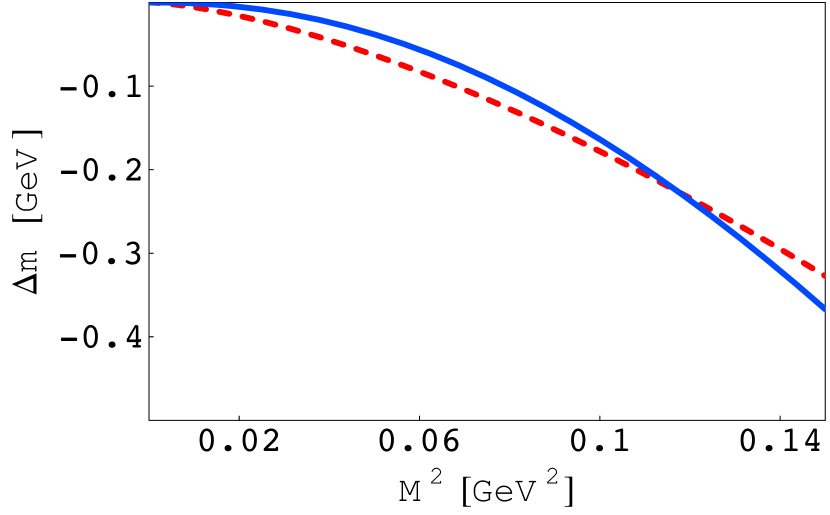
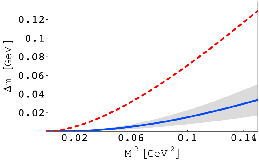
Since various so-far undetermined LECs enter the expressions for some of the higher-order $k_{i}$ it is not possible to give an accurate estimate of all terms in Eq. (11). However, the fifth-order contribution $k_{5}M^{5}\ln\frac{M}{\mu}$ is found to be $k_{5}M^{5}\ln\frac{M}{m_{N}}=-4.8\,\text{MeV}$ at the physical pion mass with $\mu=m_{N}$, while $k_{6}M^{5}=3.7\,\text{MeV}$ or $k_{6}M^{5}=-7.6\,\text{MeV}$ depending on the choice of the third-order LEC $d_{16}$ Schindler:2007dr . Equation (11) can also be used to examine the pion-mass dependence of the nucleon mass, which plays an important role in the extrapolation of lattice QCD to physical quark masses. Figure 2 shows the comparison of various terms in Eq. (11) as a function of the squared pion mass. While the right panel shows the expected suppression of the higher-order term over the whole pion-mass range, the left panel indicates that the term $k_{5}M^{5}\ln\frac{M}{\mu}$ becomes as large as $k_{2}M^{3}$ for a pion mass of roughly $M\sim 360\,\text{MeV}$. While this is not a reliable prediction of the behavior of higher-order contributions since only the leading nonanalytic parts are considered, the pion mass range at which the power counting is no longer applicable agrees with the estimates found in Refs. Meissner:2005ba ; Djukanovic:2006xc .

III.2 Probing the convergence of perturbative series

The issue of the convergence of perturbative calculations is presently of great interest in the context of chiral extrapolations of baryon properties (see, e.g., Refs. Leinweber:2003dg ; Procura:2003ig ; Beane:2004ks ). A possibility of exploring the convergence of perturbative series consists of summing up certain sets of an infinite number of diagrams by solving integral equations exactly and comparing the solutions with the perturbative contributions Djukanovic:2006xc .

Figure 3: Iterated contribution to the nucleon self energy.

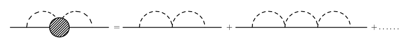
Figure 3 shows a graphical representation of an iterated contribution to the nucleon self energy originating from the Weinberg-Tomozawa term in the $\pi N$ scattering amplitude. The result is of the form Djukanovic:2006xc

$$\delta m=-\frac{3\texttt{g}_{A}^{2}}{4F^{2}}\frac{N}{D},$$ (12)

where $N$ and $D$ are closed expressions in terms of the loop functions of Eqs. (2) - (4). By expanding Eq. (12) in powers of $1/F^{2}$ one can identify the contributions of each diagram separately. Using the IR renormalization scheme and substituting $m=883$ MeV, $m_{N}=938.3$ MeV, $F=92.4$ MeV, $\texttt{g}_{A}=1.267$ and $M=139.6$ MeV one obtains

$$\delta m=-0.00233530\,{\rm MeV}=\left(-0.00230219-0.00003305-0.00000007+\ldots\right)\,{\rm MeV}\,.$$ (13)

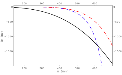
The first term in the perturbative expansion reproduces the non-perturbative result well and the higher-order corrections are clearly suppressed. Figure 4 shows $\delta m$ of Eq. (12) together with the leading contribution (first diagram in Fig. 3) and the leading non-analytic correction to the nucleon mass $\delta m_{3}=-3g_{A}^{2}M^{3}/(32\pi F^{2})$ Gasser:1987rb as functions of $M$. As can be seen from this figure, up to $M\sim 500$ MeV the non-perturbative sum of higher-order corrections is suppressed in comparison with the $\delta m_{3}$ term. Also, the leading higher-order contribution reproduces the non-perturbative result quite well. On the other hand, for $M\gtrsim 600$ MeV the higher-order contributions are no longer suppressed in comparison with $\delta m_{3}$.

Figure 4: Contributions to the nucleon mass as functions of $M$. Solid line: ${\cal O}(q^{3})$ contribution, dashed line: $\delta m$ of Eq. (12); dashed-dotted line: two-loop diagram of Fig. 3.

III.3 Electromagnetic form factors

Imposing the relevant symmetries such as translational invariance, Lorentz covariance, the discrete symmetries, and current conservation, the nucleon matrix element of the electromagnetic current operator $J^{\mu}(x)$ can be parameterized in terms of two form factors,

$$\langle N(p^{\prime})|J^{\mu}(0)|N(p)\rangle=\bar{u}(p^{\prime})\left[F_{1}^{N}(Q^{2})\gamma^{\mu}+i\frac{\sigma^{\mu\nu}q_{\nu}}{2m_{p}}F_{2}^{N}(Q^{2})\right]u(p),\quad N=p,n,$$ (14)

where $q=p^{\prime}-p$, $Q^{2}=-q^{2}$, and $m_{p}$ is the proton mass. At $Q^{2}=0$, the so-called Dirac and Pauli form factors $F_{1}$ and $F_{2}$ reduce to the charge and anomalous magnetic moment in units of the elementary charge and the nuclear magneton $e/(2m_{p})$, respectively,

$$F_{1}^{p}(0)=1,\quad F_{1}^{n}(0)=0,\quad F_{2}^{p}(0)=1.793,\quad F_{2}^{n}(0)=-1.913.$$

The Sachs form factors $G_{E}$ and $G_{M}$ are linear combinations of $F_{1}$ and $F_{2}$,

$$G_{E}^{N}(Q^{2})=F_{1}^{N}(Q^{2})-\frac{Q^{2}}{4m_{p}^{2}}F_{2}^{N}(Q^{2}),\quad G_{M}^{N}(Q^{2})=F_{1}^{N}(Q^{2})+F_{2}^{N}(Q^{2}),\quad N=p,n.$$

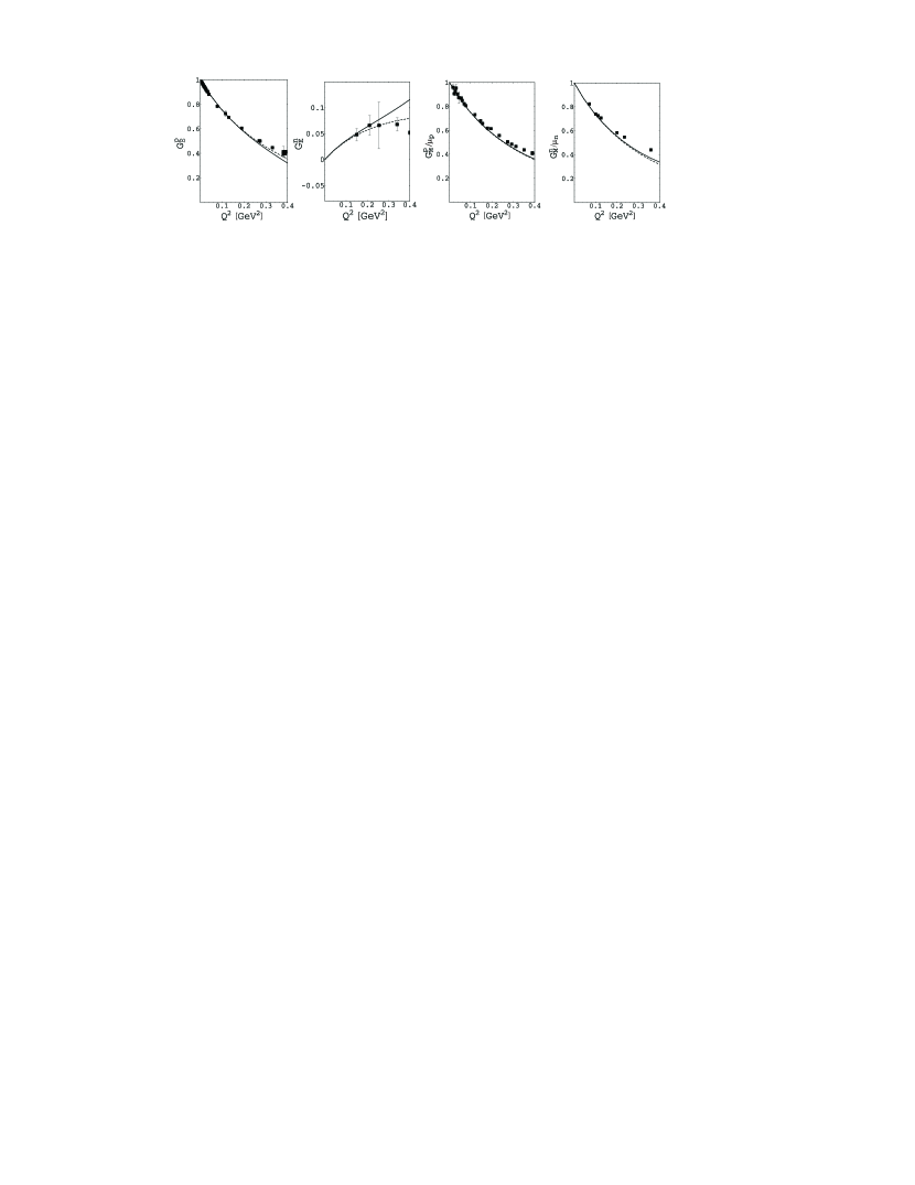
Calculations in Lorentz-invariant baryon ChPT up to fourth order fail to describe the proton and nucleon form factors for momentum transfers beyond $Q^{2}\sim 0.1\,\mbox{GeV}^{2}$ Kubis:2000zd ; Fuchs:2003ir . In Ref. Kubis:2000zd it was shown that the inclusion of vector mesons can result in the re-summation of important higher-order contributions. In Ref. Schindler:2005ke the electromagnetic form factors of the nucleon up to fourth order have been calculated in manifestly Lorentz-invariant ChPT with vector mesons as explicit degrees of freedom. A systematic power counting for the renormalized diagrams has been implemented using both the extended on-mass-shell renormalization scheme and the reformulated version of infrared regularization. The inclusion of vector mesons results in a considerably improved description of the form factors (see Fig. 5). The most dominant contributions come from tree-level diagrams, while loop corrections with internal vector meson lines are small Schindler:2005ke .

Figure 5: The Sachs form factors of the nucleon in manifestly Lorentz-invariant chiral perturbation theory at ${\cal O}(q^{4})$ including vector mesons as explicit degrees of freedom. Full lines: results in the extended on-mass-shell scheme; dashed lines: results in infrared regularization. The experimental data are taken from Ref. Friedrich:2003iz .

III.4 Axial and induced pseudoscalar form factors

Assuming isospin symmetry, the most general parametrization of the isovector axial-vector current evaluated between one-nucleon states is given by

$$\langle N(p^{\prime})|A^{\mu,a}(0)|N(p)\rangle=\bar{u}(p^{\prime})\left[\gamma^{\mu}\gamma_{5}G_{A}(Q^{2})+\frac{q^{\mu}}{2m_{N}}\gamma_{5}G_{P}(Q^{2})\right]\frac{\tau^{a}}{2}u(p),$$ (15)

where $q=p^{\prime}-p$, $Q^{2}=-q^{2}$, and $m_{N}$ denotes the nucleon mass. $G_{A}(Q^{2})$ is called the axial form factor and $G_{P}(Q^{2})$ is the induced pseudoscalar form factor. The value of the axial form factor at zero momentum transfer is defined as the axial-vector coupling constant, $g_{A}=G_{A}(Q^{2}=0)=1.2694(28)$, and is quite precisely determined from neutron beta decay. The $Q^{2}$ dependence of the axial form factor can be obtained either through neutrino scattering or pion electroproduction. The second method makes use of the so-called Adler-Gilman relation Adler:1966gd which provides a chiral Ward identity establishing a connection between charged pion electroproduction at threshold and the isovector axial-vector current evaluated between single-nucleon states (see, e.g., Ref. Bernard:2001rs ; Fuchs:2003vw for more details). The induced pseudoscalar form factor $G_{P}(Q^{2})$ has been investigated in ordinary and radiative muon capture as well as pion electroproduction (see Ref. Gorringe:2002xx for a review).

In Ref. Schindler:2006it the form factors $G_{A}$ and $G_{P}$ have been calculated in BChPT up to and including order ${\cal O}(q^{4})$. In addition to the standard treatment including the nucleon and pions, the axial-vector meson $a_{1}(1260)$ has also been considered as an explicit degree of freedom. The inclusion of the axial-vector meson effectively results in one additional low-energy coupling constant which has been determined by a fit to the data for $G_{A}(Q^{2})$. The inclusion of the axial-vector meson results in an improved description of the experimental data for $G_{A}$ (see Fig. 6), while the contribution to $G_{P}$ is small.

Figure 6: Left panel: Axial form factor $G_{A}$ in manifestly Lorentz-invariant ChPT at ${\cal O}(q^{4})$ including the axial-vector meson $a_{1}(1260)$ explicitly. Full line: result in infrared renormalization, dashed line: dipole parametrization. The experimental data are taken from Ref. Bernard:2001rs . Right panel: The induced pseudoscalar form factor $G_{P}$ at ${\cal O}(q^{4})$ including the axial-vector meson $a_{1}(1260)$ explicitly. Full line: result with axial-vector meson; dashed line: result without axial-vector meson. One can clearly see the dominant pion pole contribution at $Q^{2}\approx-M_{\pi}^{2}$.

IV Complex-mass scheme and effective field theory

In Sec. III.3 we saw how the inclusion of virtual vector mesons generates an improved description of the electromagnetic form factors, for which ordinary chiral perturbation theory does not produce sufficient curvature. So far the inclusion of virtual vector mesons has been restricted to low-energy processes in which the vector mesons cannot be generated explicitly. However, one would also like to investigate the properties of hadronic resonances such as their masses and widths as well as their electromagnetic properties. An extension of chiral effective field theory to the momentum region near the complex pole corresponding to the vector mesons was proposed in Ref. Djukanovic:2009zn , in which the power-counting problem was addressed by applying the complex-mass scheme (CMS) Stuart:1990 ; Denner:1999gp ; Denner:2005fg ; Denner:2006ic to the effective field theory. Since the $\rho$ mass is not treated as a small quantity, the presence of large external four-momenta, e.g., in terms of the zeroth component, leads to a considerable complication regarding the power counting of loop diagrams. To assign a chiral order to a given diagram it is first necessary to investigate all possibilities how the external momenta could flow through the internal lines of that diagram. Next, when assigning powers to propagators and vertices, one needs to determine the chiral order for a given flow of external momenta. Finally, the smallest order resulting from the various assignments is defined as the chiral order of the given diagram. The application of the CMS to the renormalization of loop diagrams amounts to splitting the bare parameters of the Lagrangian into renormalized parameters and counter terms and choosing the renormalized masses as the complex poles of the dressed propagators in the chiral limit, $M_{R}^{2}=(M_{\chi}-i\Gamma_{\chi}/2)^{2}$. The result for the chiral expansion of the pole mass and the width of the $\rho$ meson to ${\cal O}(q^{4})$ reads Djukanovic:2009zn

$$M_{\rho}^{2} = M_{\chi}^{2}+c_{x}M^{2}-\frac{g_{\omega\rho\pi}^{2}M^{3}M_{\chi}}{24\pi}$$ (16)

$$+\frac{M^{4}}{32\pi^{2}F^{2}}\left(3-2\,\ln\frac{M^{2}}{M_{\chi}^{2}}\right)+\frac{g_{\omega\rho\pi}^{2}M^{4}}{32\pi^{2}}\left(1-\ln\frac{M^{2}}{M_{\chi}^{2}}\right)\,,$$

$$\Gamma = \Gamma_{\chi}+\frac{\Gamma_{\chi}^{3}}{8M_{\chi}^{2}}-\frac{c_{x}\Gamma_{\chi}M^{2}}{2M_{\chi}^{2}}-\frac{g_{\omega\rho\pi}^{2}M^{3}\Gamma_{\chi}}{48\pi\,M_{\chi}}+\frac{M^{4}}{16\,\pi\,F^{2}M_{\chi}}\,.$$ (17)

Here, $M^{2}$ is the lowest-order expression for the squared pion mass, $F$ the pion-decay constant in the chiral limit, $c_{x}$ a low-energy coupling constant of the $\pi\rho$ Lagrangian, and $g_{\omega\rho\pi}$ a coupling constant. The nonanalytic terms of Eq. (16) agree with the results of Ref. Leinweber:2001ac . Both mass $M_{\chi}$ and width $\Gamma_{\chi}$ in the chiral limit are input parameters in this approach. The numerical importance of the different contributions has been estimated using

$$F=0.092\,{\rm GeV},\quad M=0.139\,{\rm GeV}\,,\quad g_{\omega\rho\pi}=16\,{\rm GeV^{-1}},\quad M_{\chi}\approx M_{\rho}=0.78\,{\rm GeV},$$

resulting in the expansion (units of GeV² and GeV, respectively)

$$M_{\rho}^{2} = M_{\chi}^{2}+0.019\,c_{x}-0.0071+0.0014+0.0013\,,$$

$$\Gamma \approx \Gamma_{\chi}+0.21\,\Gamma_{\chi}^{3}-0.016\,c_{x}\Gamma_{\chi}-0.0058\,\Gamma_{\chi}+0.0011\,.$$ (18)

For pion masses larger than $M_{\rho}/2$ the $\rho$ meson becomes a stable particle. For such values of the pion mass the series of Eq. (17) should diverge. Along similar lines, Ref. Djukanovic:2009gt contains a calculation of the mass and the width of the Roper resonance using the CMS.

V Conclusion

In the baryonic sector new renormalization conditions have reconciled the manifestly Lorentz-invariant approach with the standard power counting. We have discussed some results of a two-loop calculation of the nucleon mass. The inclusion of vector and axial-vector mesons as explicit degrees of freedom leads to an improved phenomenological description of the electromagnetic and axial form factors, respectively. Work on the application to electromagnetic processes such as Compton scattering and pion production is in progress. When describing resonances in perturbation theory, one needs to take their finite widths into account. The CMS has opened a new window for describing unstable particles in EFT with a consistent power counting.