Correlations between CME Parameters and Sunspot Activity

Abstract

Smoothed monthly mean coronal mass ejection (CME) parameters (speed, acceleration, central position angle, angular width, mass and kinetic energy) for Cycle 23 are cross-analyzed, showing a high correlation between most of them. The CME acceleration ($a$) is found to be highly correlated with the reciprocal of its mass ($M$), with a correlation coefficient $r=0.899$. The force ($Ma$) to drive a CME is found to be well anti-correlated with the sunspot number ($R_{\mathrm{z}}$), $r=-0.750$. The relationships between CME parameters and $R_{\mathrm{z}}$ can be well described by an integral response model with a decay time scale of about 11 months. The correlation coefficients of CME parameters with the reconstructed series based on this model ($\overline{r}_{\mathrm{f1}}=0.886$) are higher than the linear correlation coefficients of the parameters with $R_{\mathrm{z}}$ ($\overline{r}_{\mathrm{0}}=0.830$). If a double decay integral response model is used (with two decay time scales of about 6 and 60 months), the correlations between CME parameters and $R_{\mathrm{z}}$ improve ($\overline{r}_{\mathrm{f2}}=0.906$). The time delays between CME parameters with respect to Rz are also well predicted by this model (19/22 = 86%); the average time delays are 19 months for the reconstructed and 22 months for the original time series. The model implies that CMEs are related to the accumulation of solar magnetic energy. The relationships found can help to understand the mechanisms at work during the solar cycle.

1 Introduction

A coronal mass ejection (CME) is a striking manifestation of solar activity seen in the solar corona (e.g., Gosling, 1993; Webb & Howard, 1994). In a typical CME, billions of tons of solar magnetized plasma with energy above $10^{32}$ erg can be pushed into the space (e.g., Vourlidas et al., 2000; Gopalswamy et al., 2000; Falconer et al., 2002). CMEs may cause strong interplanetary disturbances and geomagnetic storms (Gonzalez et al., 1994; Gopalswamy, 2010). Very high-energy (GeV) particles generated by CME-driven shocks with large Mach numbers are hazardous to our modern highly technological equipments (e.g., Roussev et al., 2003; Lee, 2005).

CMEs originate from large-scale closed magnetic field structures related to active regions with or without filaments or to quiescent filaments (Munro et al., 1979; Chen & Shibata, 2000; Forbes et al., 2006; Gopalswamy, 2006). The magnetic field in the lower corona is a key element in the genesis of CMEs (e.g., Forbes et al., 2006). The fastest CMEs originate because of an instability of strong magnetic fields ($\geq$ 100 G), generally in active regions with sunspots (Falconer et al., 2002; Gopalswamy et al., 2003, 2010) while the high latitude CMEs are mainly related to quiescent prominence eruptions (Gopalswamy et al., 2003). Sunspots represent one of the most obvious manifestations of solar magnetic activity (Moradi et al., 2010) and its number and characteristics can be considered as a measure of the energy supplied to the corona (Temmer et al., 2003). Studying the relationships between CME parameters and solar activity, represented by the international relative sunspot number ($R_{\mathrm{z}}$), can be useful to understand the mechanisms at work during the solar activity cycle (Sakurai, 1976; Antiochos et al., 1999; Rust, 2003; Wang et al., 2000; Mittal & Narain, 2010; Kilcik et al., 2011).

Since the first CME was discovered in data from the Naval Research Laboratory (NRL) coronagraph mounted on the Orbiting Solar Observatory-7 (OSO-7) NASA satellite (Koomen et al., 1975), the properties of CMEs have been carefully examined, particularly after the advent of the Large Angle and Spectrometric Coronagraph (LASCO, Brueckner et al., 1995; Domingo et al., 1995) on board the Solar and Heliospheric Observatory (SOHO).

Some CME parameters follow the solar cycle rather well while others do not (Gopalswamy et al., 2003; Kane, 2006; Ivanov et al., 2009; Gopalswamy, 2010; Gopalswamy et al., 2010; Gerontidou et al., 2010, and references therein). The number of CMEs per day shows a strong dependence on the solar cycle (Hildner et al., 1976; St. Cyr et al., 2000; Gopalswamy et al., 2003; Gopalswamy, 2006, 2010; Cremades & St. Cyr, 2007; Gerontidou et al., 2010). The CME speeds have also been found to follow the solar cycle (Gopalswamy et al., 2003; Gopalswamy, 2010; Cremades & St. Cyr, 2007). However, the CME mass and angular width do not exhibit a significant variation with the solar cycle (Cremades & St. Cyr, 2007). The number of CMEs was shown to follow well the sunspot number only during the rising phase of Solar Cycle 23, while there were large fluctuations in the maximum and the declining phase of this solar cycle (Gerontidou et al., 2010; Gopalswamy, 2010). The CME sources associated with active regions follow the butterfly diagram and appear at lower latitudes as the cycle progresses, while those related to filaments outside active regions tend to migrate towards higher latitudes (Gopalswamy et al., 2003; Cremades & St. Cyr, 2007; Gopalswamy et al., 2010, and references therein).

It is well known that solar flares (e.g., Aschwanden, 1994; Temmer et al., 2003), CMEs (Gonzalez & Tsurutani, 1987; Tsurutani et al., 2006; Ramesh, 2010; Kilcik et al., 2011), and geomagnetic activities (Wilson, 1990; Echer et al., 2004; Ramesh, 2010; Kilcik et al., 2011) often lag behind sunspot activity ($R_{\mathrm{z}}$) from several months to a few years. To have a better understanding of the relationship between solar ($R_{\mathrm{z}}$) and geomagnetic activity ($aa$ index), Du (2011a) proposed an integral response model to describe better this relationship. It is found that the correlation between $aa$ and $R_{\mathrm{z}}$ yielded by this model is much higher than that found by a simple point-point correspondence. Some phenomena can be explained by this model, such as the significant increase in the $aa$ index over the 20th century (Feynman & Crooker, 1978; Clilverd et al., 1998; Demetrescu & Dobrica, 2008; Lukianova et al., 2009), the longer lag times at solar (cycle) maximum than at solar minimum (Wilson, 1990; Wang et al., 2000; Echer et al., 2004), and the decreasing trend in the correlation between $aa$ and $R_{\mathrm{z}}$ (Borello-Filisetti et al., 1992; Mussino et al., 1994; Kishcha et al., 1999; Echer et al., 2004; Du, 2011b).

This paper investigates in detail the relationships and time delays between CME parameters and sunspot numbers ($R_{\mathrm{z}}$). The CME parameters (speed, acceleration, central position angle, angular width, mass and kinetic energy) and the methods used in this paper are described in Section 2. The linear cross-correlations among the above parameters and their dependencies on $R_{\mathrm{z}}$ are first analyzed in Section 3.1. An integral response model (Du, 2011a) is then used to study the relationships and time delays between the CME parameters and $R_{\mathrm{z}}$ in Section 3.2. In this model, the output depends not only on the present input, but also on past values. In a second step, this model is modified and the relationships between the CME parameters and $R_{\mathrm{z}}$ improve (see Section 3.3). Finally, our conclusions are discussed and summarized in Section 4.

2 Data and Methods

The data used in this study comprise monthly-mean sunspot numbers ($R_{\mathrm{z}}$) produced by the Solar Influences Data Analysis Center (SIDC, http://www.sidc.be/sunspot-data/) and CME parameters obtained from the SOHO/LASCO CME catalog identified since 1996 (http://cdaw.gsfc.nasa.gov/, see e.g., Gopalswamy et al., 2000; Yashiro et al., 2004). The following CME parameters are analyzed:

1. $V_{1}$: linear speed obtained by fitting a straight line to the height-time measurements (in units of km s^-1).

2. $V_{20}$: initial speed obtained by fitting a parabola to the height-time measurements.

3. $V_{2}$: final speed at the time of final height measurements by fitting a parabola.

4. $V_{20R}$: speed obtained as above but evaluated when the CME is at a height of 20$R_{\odot}$ (solar radii).

5. $a$: acceleration obtained by fitting a parabola to the height-time measurements (in km s^-2).

6. $W$: angular width in the plane of the sky (in degrees).

7. $P_{0}$: central position angle (CPA, in degrees), from solar north (counterclockwise).

8. $P_{\mathrm{m}}$: position angle (in degrees) at the fastest portion of the leading edge (Yashiro et al., 2004).

9. $M$: mass (in grams).

10. $E$: kinetic energy (in ergs), obtained from the linear speed ($V_{1}$) and the CME mass ($M$).

The above parameters are first integrated over each day and, then, averaged over each month to obtain the monthly-means of integrated daily parameters. Such a treatment aims to analyze the total contribution of CMEs over a month. Ideally, CME projection effects should be corrected in advance to accurately measure the parameters (Cremades & St. Cyr, 2007; Ivanov et al., 2009; Gopalswamy, 2010). As doing this for all CMEs is a difficult task and there is a small number of CMEs with $W>120^{\rm o}$ (11%, Gopalswamy et al., 2010), projection effects have not been corrected in this study. In addition, we do not consider the N-S asymmetry of the position angles ($P_{0}$ and $P_{\mathrm{m}}$); that is, we use the values of position angles in terms of co-latitude — computed from the solar North pole for the northern hemisphere and from the solar South pole for the southern hemisphere. The $P_{0}$ and $P_{\mathrm{m}}$ values may be greater than $90^{\mathrm{o}}$ due to the integral contributions of many CMEs in a day. To filter out high frequency variations in the data, the parameters are smoothed with the standard 13-month running mean technique (with half weights at the two ends). The results are shown in Fig. 1 for the period July 1996 to December 2008 (the time of solar minimum preceding Cycle 24).

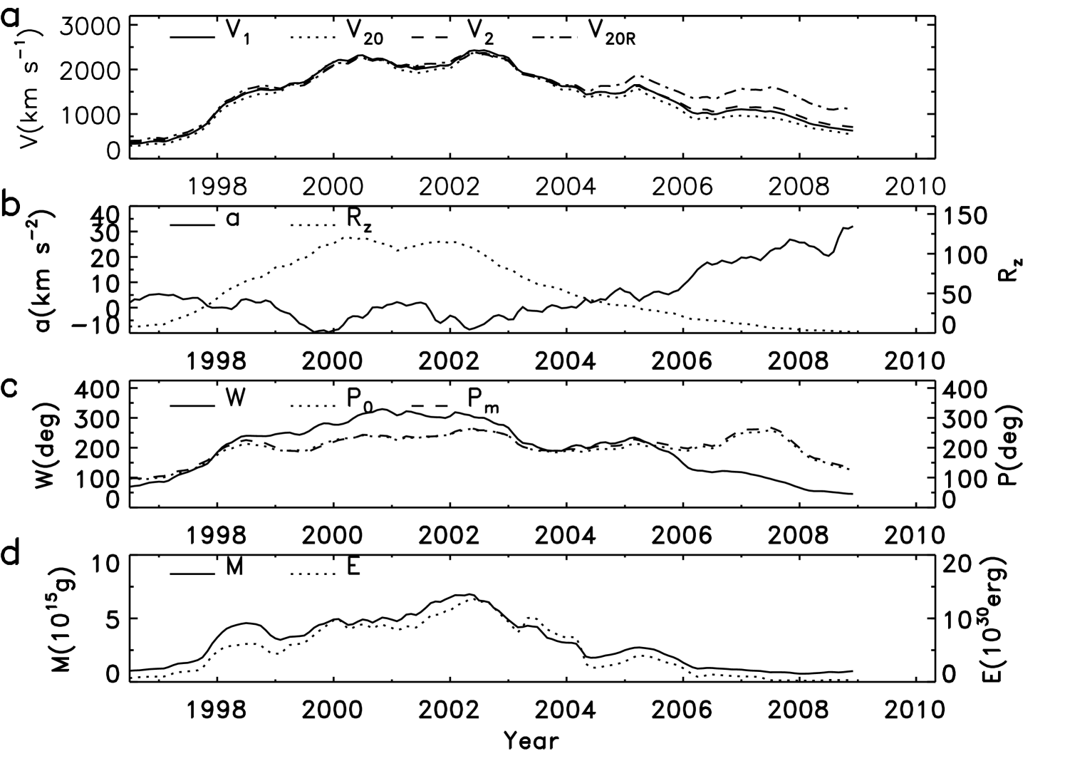
Figure 1: (a) Smoothed monthly mean $V_{1}$ (solid line), $V_{20}$ (dotted line), $V_{\mathrm{2}}$ (dashed line), and $V_{\mathrm{20R}}$ (dash-dotted line) from July 1996 to December 2008. (b) $a$ (solid line) and $R_{\mathrm{z}}$ (dotted line). (c) $W$ (solid line), $P_{0}$ (dotted line), and $P_{\mathrm{m}}$ (dashed line). (d) $M$ (solid line) and $E$ (dotted line).

3 Results

3.1 Correlations between CME Parameters

The relationships among CME parameters and other phenomena have been well examined in the past. For example, faster CMEs tend to be wider (e.g., Gopalswamy, 2010; Gopalswamy et al., 2010), with a correlation coefficient of $r=0.44$ between $V_{1}$ and $W$ for $V_{1}>900$ km s^-1 (Yashiro et al., 2004), and wider CMEs generally have greater mass contents, $M\propto W^{1.3}$ (e.g., Gopalswamy, 2010; Aarnio et al., 2011). CMEs with the above-average speeds (466 km s^-1) decelerate, while those with speeds well below the average accelerate (Gopalswamy et al., 2000; Yashiro et al., 2004; Gopalswamy, 2006; Gopalswamy et al., 2010; Aarnio et al., 2011). Strong CMEs are often accompanied by solar flares, type II radio bursts, energetic particles, and geomagnetic storms (e.g., Gonzalez et al., 1994; Roussev et al., 2003; Gopalswamy, 2010).

Table 1: Correlation coefficients between CME parameters.

$r$	$V_{1}$	$V_{\mathrm{20}}$	$V_{\mathrm{2}}$	$V_{\mathrm{20R}}$	$-a$	$W$	$P_{\mathrm{0}}$	$P_{\mathrm{m}}$	$M$	$E$	$R_{\mathrm{z}}$
$V_{1}$	1.	0.998	0.998	0.956	0.670	0.929	0.771	0.724	0.887	0.912	0.894
$V_{\mathrm{20}}$	0.998	1.	0.994	0.942	0.696	0.932	0.742	0.690	0.893	0.921	0.908
$V_{\mathrm{2}}$	0.998	0.994	1.	0.967	0.637	0.923	0.794	0.749	0.877	0.899	0.888
$V_{\mathrm{20R}}$	0.956	0.942	0.967	1.	0.436	0.820	0.886	0.853	0.768	0.794	0.768
$-a$	0.670	0.696	0.637	0.436	1.	0.805	0.205	0.147	0.791	0.793	0.795
$W$	0.929	0.932	0.923	0.820	0.805	1.	0.630	0.588	0.926	0.892	0.943
$P_{\mathrm{0}}$	0.771	0.742	0.794	0.886	0.205	0.630	1.	0.994	0.569	0.563	0.551
$P_{\mathrm{m}}$	0.724	0.690	0.749	0.853	0.147	0.588	0.994	1.	0.518	0.502	0.485
$M$	0.887	0.893	0.877	0.768	0.791	0.926	0.569	0.518	1.	0.971	0.936
$E$	0.912	0.921	0.899	0.794	0.793	0.892	0.563	0.502	0.971	1.	0.916

In this section, we simply analyze the correlation coefficients between the CME parameters, as listed in Table 1. It is seen that these values are very high, from 0.77 to 0.99, except for related to $a$, $P_{\mathrm{0}}$ and $P_{\mathrm{m}}$. The following can be noted:

1. $V_{1}$ (solid line), $V_{20}$ (dotted line), $V_{2}$ (dashed line), and $V_{\mathrm{20R}}$ (dash-dotted line) in Fig. 1a are highly cross-correlated with correlation coefficients in the range from $r=0.956$ to 0.998. So, if one of these speeds is well correlated with any other parameter (e.g., $R_{\rm z}$), the others will also be.

2. $a$ (solid line in Fig. 1b) is inversely correlated with $V_{1}$, $V_{20}$, $V_{2}$, and $V_{\mathrm{20R}}$, $r=-0.436$ to $-0.696$, implying that CMEs with faster speeds tend to decelerate faster (Gopalswamy et al., 2000; Yashiro et al., 2004; Gopalswamy, 2006; Gopalswamy et al., 2010; Aarnio et al., 2011).

3. $W$ (solid line in Fig. 1c) is well correlated with $V_{1}$, $V_{20}$, $V_{2}$, and $V_{\mathrm{20R}}$, $r=0.820$ to $0.932$, suggesting that CMEs with faster speeds tend to be wider (Yashiro et al., 2004; Gopalswamy, 2010; Gopalswamy et al., 2010).

4. $W$ is well anti-correlated with $a$, $r=-0.805$, suggesting that wider CMEs tend to decelerate faster.

5. Both $P_{\mathrm{m}}$ (dotted line) and $P_{0}$ (dashed line) in Fig. 1c are well correlated with $V_{1}$, $V_{20}$, $V_{2}$, and $V_{\mathrm{20R}}$, $r=0.690$ to 0.886, suggesting that faster CMEs tend to be closer to the solar equator.

6. $P_{\mathrm{m}}$ is highly correlated with $P_{0}$, $r=0.994$, with the former slightly larger than the latter ($5.1^{\mathrm{o}}$).

7. $W$ is positively correlated with $P_{0}$ and $P_{\mathrm{m}}$, $r=0.630$ and 0.588, respectively, suggesting that wider CMEs tend to be closer to the solar equator.

8. $a$ is almost uncorrelated with both $P_{0}$ and $P_{\mathrm{m}}$, $r=-0.205$ and $-0.147$, respectively.

9. $M$ (solid line in Fig. 1d) is well correlated with $V_{1}$, $V_{20}$, $V_{2}$, and $V_{\mathrm{20R}}$, $r=0.768$ to $0.893$, suggesting that faster CMEs carry more mass outward.

10. $M$ is highly correlated with $W$, $r=0.926$, suggesting that wider CMEs carry more mass outward (Gopalswamy, 2010; Aarnio et al., 2011).

11. $M$ is correlated with $P_{0}$ and $P_{\mathrm{m}}$, $r=0.569$ and $0.518$, respectively, suggesting that CMEs closer to the solar equator tend to carry more mass outward.

12. $E$ (dotted line in Fig. 1d) is highly correlated with $M$, $V_{1}$, $V_{20}$, $V_{2}$, and $V_{\mathrm{20R}}$ since $E=MV^{2}/2$ (Vourlidas et al., 2000).

13. $E$ is well correlated with $W$, $r=0.892$, suggesting that wider CMEs carry away more energy (Gopalswamy, 2010; Aarnio et al., 2011).

14. $E$ is correlated with $P_{0}$ and $P_{\mathrm{m}}$, $r=0.563$ and $0.502$, respectively, suggesting that CMEs closer to the solar equator tend to carry away more energy.

15. The correlation coefficients of $P_{\mathrm{m}}$ are systemically lower than those of $P_{0}$ with other parameters, which may be due to a more non-linear behavior close to the leading edge.

16. The parameters are well correlated with $R_{\mathrm{z}}$ (dotted line in Fig. 1b), except for an anti-correlation of $a$ with $R_{\mathrm{z}}$.

17. $a$ is well anti-correlated with $M$ ($r=-0.791$).

In summary, CMEs with faster speeds tend to be wider, to be closer to the solar equator, to decelerate faster, and to carry more mass and energy outward. For other properties of CMEs, the readers can refer to excellent reviews in the literature (Gopalswamy, 2006; Cremades & St. Cyr, 2007; Gopalswamy, 2010; Gerontidou et al., 2010).

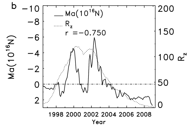
Figure 2: (a) $a$ (solid line) is well correlated with $1/M$ (dotted line), $r=0.899$. (b) $Ma$ (solid line) is well anti-correlated with $R_{\mathrm{z}}$ (dotted line), $r=-0.750$.

Aarnio et al. (2011) pointed out that the mass of a CME is unrelated to its acceleration. However, it is shown that $a$ is well anti-correlated with $M$ ($r=-0.791$). In fact, $a$ is highly correlated with the reciprocal of the mass $1/M$ ($r=0.899$), as shown in Fig. 2a. It seems to suggest that the CME motion approximately obeys Newton’s second law. Thus, $F=Ma$ can be understood as the ‘force’ to drive a CME. This force is found to be well anti-correlated with $R_{\mathrm{z}}$ ($r=-0.750$), as shown in Fig. 2b for $Ma$ (solid line) and $R_{\mathrm{z}}$ (dotted line). $F>0$ around the solar minima, $F=0$ around $R_{\mathrm{z}}\sim 41$, while there is not a definite sign of $F$ around the solar maximum. It is well known that there are two peaks in $R_{\mathrm{z}}$ for Cycle 23, the first one (120.8 in April 2000) being higher than the second one (115.5 in November 2001). One can see in Fig. 2b that there are also two peaks in $-(Ma)$ for Cycle 23, the first one ($4.6\times 10^{16}$ in December 1999) being lower than the second one ($5.9\times 10^{16}$ in May 2002). Around the two peaks in $R_{\mathrm{z}}$, $F<0$, while coincident with the gap between both peaks, $F>0$.

3.2 Relationships between CME Parameters and $R_{\mathrm{z}}$ Described by an Integral Response Model

It is well known that the occurrence of the largest CMEs tends to peak some years after the sunspot maximum (Gonzalez & Tsurutani, 1987; Tsurutani et al., 2006; Ramesh, 2010; Kilcik et al., 2011). To explain the time delays between CME parameters with respect to $R_{\mathrm{z}}$, in this section, we employ the following integral response model (Du, 2011a), hereafter Model I, to analyze the relationships between some typical CME parameters ($V_{20}$, $W$, $P_{0}$ and $E$) and $R_{\mathrm{z}}$,

$$\begin{array}[]{lrl}y(t)&=&D\int_{t^{\prime}=-\infty}^{t}x(t^{\prime})e^{-(t-t^{\prime})/\tau}dt^{\prime}+y_{0},\\ &&{(\rm Model\ I)}\\ \end{array}$$ (3)

where $y$ represents one of the CME parameters and $x=R_{\mathrm{z}}$, $y_{0}$ is a constant, $D$ is called the ‘dynamic response factor’, and $\tau$ is called the ‘response time scale’ of $y$ to $x$. Figure 3a illustrates the reconstructed series ($V_{\mathrm{20f}}$, dotted line) based on this model for $y=V_{20}$ (solid line) and $x=R_{\mathrm{z}}$ (dashed line).

Figure 3: (a) $V_{20}$ (solid line), $R_{\mathrm{z}}$ (dashed line), and the reconstructed series ($V_{\mathrm{20f}}$, dotted line) by Model I (Equation (3)). The correlation coefficients of $V_{20}$ with $R_{\mathrm{z}}$ and $V_{\mathrm{20f}}$ are $r_{0}=0.908$ and $r_{\mathrm{f}}=0.966$, respectively. (b) Similar results for the relationship between $W$ (solid line) and $R_{\mathrm{z}}$ (dashed line). The correlation coefficients of $W$ with $R_{\mathrm{z}}$ and the reconstructed series $W_{\mathrm{f}}$ (dotted line) are $r_{0}=0.943$ and $r_{\mathrm{f}}=0.950$, respectively. (c) Relationship between $P_{0}$ (solid line) and $R_{\mathrm{z}}$ (dashed line). The correlation coefficients of $P_{0}$ with $R_{\mathrm{z}}$ and the reconstructed series $P_{\mathrm{0f}}$ (dotted line) are $r_{0}=0.551$ and $r_{\mathrm{f}}=0.679$, respectively. (d) Relationship between $E$ (solid line) and $R_{\mathrm{z}}$ (dashed line). The correlation coefficients of $E$ with $R_{\mathrm{z}}$ and the reconstructed series $E_{\mathrm{f}}$ (dotted line) are $r_{0}=0.916$ and $r_{\mathrm{f}}=0.947$, respectively.

It is apparent in Fig. 3a that the reconstructed series ($V_{\mathrm{20f}}$) reflects well the profile of $V_{20}$. The correlation coefficient between $V_{20}$ and $V_{\mathrm{20f}}$ ($r_{\mathrm{f}}=0.966$) is higher than the linear correlation coefficient between $V_{20}$ and $R_{\mathrm{z}}$ ($r_{0}=0.908$). The fitted parameters of this model are listed in Table 2, in which $\sigma$ refers to the standard deviation.

Table 2: Fitted parameters of the integral response model (Equation (3)).

$y$-$x$	$D$	$\tau$	$y_{0}$	$\sigma$	$r_{0}$	$r_{\mathrm{f}}$
$V_{20}$-$R_{\mathrm{z}}$	1.66	8.8	549	159.9	0.908	0.966
$W$-$R_{\mathrm{z}}$	0.558	3.1	87.0	26.9	0.943	0.950
$P_{0}$-$R_{\mathrm{z}}$	0.0381	24.7	150	31.4	0.551	0.679
$E/10^{30}$-$R_{\mathrm{z}}$	0.0133	6.6	$-0.09$	1.26	0.916	0.947
Average		10.8			0.830	0.886

Figure 3b depicts the reconstructed series ($W_{\mathrm{f}}$, dotted line) based on Model I for $y=W$ (solid line) and $x=R_{\mathrm{z}}$ (dashed line). The correlation coefficient between $W$ and $W_{\mathrm{f}}$ ($r_{\mathrm{f}}=0.950$) is slightly higher than that between $W$ and $R_{\mathrm{z}}$ ($r_{0}=0.943$). Similarly, the correlation coefficient between $P_{0}$ and the reconstructed series $P_{\mathrm{0f}}$ (dotted line) based on Model I ($r_{\mathrm{f}}=0.679$) is higher than that between $P_{0}$ and $R_{\mathrm{z}}$ ($r_{0}=0.551$; see Fig. 3c). The correlation coefficient between $E$ and the reconstructed series ($E_{\mathrm{f}}$, dotted line) based on Model I ($r_{\mathrm{f}}=0.947$) is higher than that between $E$ and $R_{\mathrm{z}}$ ($r_{0}=0.916$, see Fig. 3d). The above results are listed in Table 2, in which the last row indicates the relevant averages. The average ‘response time scale’ is $\overline{\tau}=10.8$ months. The correlation coefficients increased from 0.830 to 0.886 in average when using Model I. Therefore, Model I can better describe the relationships between CME parameters and $R_{\mathrm{z}}$.

In Model I, $y_{0}$ is a constant, representing the part of CMEs that are uncorrelated with $R_{\mathrm{z}}$ (related to variability of other solar phenomena), $D$ is the ‘dynamic response factor’ of $y$ (a CME parameter) to $x(R_{\mathrm{z}}$), representing the initial efficiency of CMEs ($\partial y/\partial x|_{t^{\prime}=t}$), and $\tau$ is the ‘response time scale’ of $y$ to $x$, representing that an input (solar activity) may affect the output in the subsequent time period of about $\tau$ (months) according to an exponential decay factor ($e^{-(t-t^{\prime})/\tau}$). It implies that CMEs are related to the previous accumulation of solar magnetic energy. As is well known, the upper chromospheric activity indices tend to lag behind the sunspot number by one to several months, depending on the index, which was interpreted in terms of active regions evolving from the photosphere upward (Bachmann & White, 1994; Aschwanden, 1994; Temmer et al., 2003). Various solar magnetic activities evolve from the photosphere to upper chromosphere with different speeds and times. On average, the long-term evolution times (or periodicities) and the above lag times are reflected in the ‘response time scale’ ($\overline{\tau}\approx 11$ months).

3.3 Relationships between CME Parameters and $R_{\mathrm{z}}$ via a Double Decay Integral Response Model

As there are often two (or three) peaks in several parameters associated to solar activity (Gnevyshev, 1967; Feminella & Storini, 1997) or CMEs (Gonzalez & Tsurutani, 1987; Yashiro et al., 2004; Tsurutani et al., 2006; Kane, 2006; Cremades & St. Cyr, 2007; Ramesh, 2010), we use the following double decay model (Model II, hereafter),

$$\begin{array}[]{lrl}y(t)&=&\int_{t^{\prime}=-\infty}^{t}x(t^{\prime})\left[D_{1}e^{-(t-t^{\prime})/\tau_{1}}\right.\\ &&+\left.D_{2}e^{-(t-t^{\prime})/\tau_{2}}\right]dt^{\prime}+y_{0},\\ &&{(\rm Model\ II)}\\ \end{array}$$ (7)

to better describe the relationships between the CME parameters and $R_{\mathrm{z}}$. The results based on Model II are shown in Fig. 4 and Table 3.

Figure 4: Similar to Fig. 3 but using Model II (Equation (7)). (a) The correlation coefficient of $V_{20}$ (solid line) with the reconstructed series $V_{\mathrm{20f}}$ (dotted line) from $R_{\mathrm{z}}$ (dashed line) by Model II is now $r_{\mathrm{f}}=0.980$. The lag time of $V_{20}$ ($V_{\mathrm{20f}}$) with respect to $R_{\mathrm{z}}$ at the peak of Cycle 23 is $L_{0}=28$ ($L_{\mathrm{f}}=23$ months) months. (b) The correlation coefficient of $W$ (solid line) with the reconstructed series $W_{\mathrm{f}}$ (dotted line) from $R_{\mathrm{z}}$ (dashed line) by Model II is now $r_{\mathrm{f}}=0.954$. The lag time of $W$ ($W_{\mathrm{f}}$) with respect to $R_{\mathrm{z}}$ is $L_{0}=7$ ($L_{\mathrm{f}}=3$ months) months. (c) The correlation coefficient of $P_{0}$ (solid line) with the reconstructed series $P_{\mathrm{0f}}$ (dotted line) from $R_{\mathrm{z}}$ (dashed line) by Model II is now $r_{\mathrm{f}}=0.734$. The lag time of $P_{\mathrm{0}}$ ($P_{\mathrm{0f}}$) with respect to $R_{\mathrm{z}}$ is $L_{0}=25$ ($L_{\mathrm{f}}=27$ months) months. (d) The correlation coefficient of $E$ (solid line) with the reconstructed series $E_{\mathrm{f}}$ (dotted line) from $R_{\mathrm{z}}$ (dashed line) by Model II is now $r_{\mathrm{f}}=0.954$. The lag time of $E$ ($E_{\mathrm{f}}$) with respect to $R_{\mathrm{z}}$ is $L_{0}=26$ ($L_{\mathrm{f}}=22$ months) months.

One can see in Fig. 4a that the correlation coefficient of $y=V_{20}$ (solid line) with the reconstructed series $V_{\mathrm{20f}}$ (dotted line) from $x=R_{\mathrm{z}}$ (dashed line) by Model II is now $r_{\mathrm{f}}=0.980$, slightly higher than that of $V_{20}$ with the reconstructed series based on Model I in Fig. 3a (0.966). The lag time of $V_{20}$ with respect to $R_{\mathrm{z}}$ ($L_{0}=28$ months) is well predicted by this model ($L_{\mathrm{f}}=23$ months).

Table 3: Fitted parameters of the double decay integral response model (Equation (7)).

$y$-$x$	$D_{1}$	$\tau_{1}$	$D_{2}$	$\tau_{2}$	$y_{0}$	$\sigma$	$r_{0}$	$r_{\mathrm{f}}$	$L_{0}$	$L_{\mathrm{f}}$
$V_{20}$-$R_{\mathrm{z}}$	6.30	1.6	0.13	75.6	286	123.5	0.908	0.980	28	23
$W$-$R_{\mathrm{z}}$	0.94	1.4	0.0092	34.9	74.9	26.6	0.943	0.954	7	3
$P_{0}$-$R_{\mathrm{z}}$	0.0811	5.0	0.0167	82.9	121	29.8	0.551	0.734	25	27
$E/10^{30}$-$R_{\mathrm{z}}$	0.0092	17.0	$-0.0022$	45.3	1.12	1.17	0.916	0.954	26	22
Average		10.8			0.830	0.886

Figure 4b illustrates the results for $y=W$ (solid line) and $x=R_{\mathrm{z}}$ (dashed line). The correlation coefficient of $W$ with the reconstructed series $W_{\mathrm{f}}$ (dotted line) by Model II is now $r_{\mathrm{f}}=0.954$, slightly higher than that of $W$ with the reconstructed series based on Model I in Fig. 3b ($0.950$). About half of the lag time of $V_{20}$ with respect to $R_{\mathrm{z}}$ ($L_{0}=7$ months) is predicted by this model ($L_{\mathrm{f}}=3$ months). In Fig. 4c, the correlation coefficient of $P_{0}$ (solid line) with the reconstructed series $P_{\mathrm{0f}}$ (dotted line) from $R_{\mathrm{z}}$ (dashed line) by Model II is now $r_{\mathrm{f}}=0.734$, slightly higher than that of $P_{0}$ with the reconstructed series based on Model I in Fig. 3c (0.679). The lag time of $V_{20}$ with respect to $R_{\mathrm{z}}$ ($L_{0}=25$ months) is approximately predicted by this model ($L_{\mathrm{f}}=27$ months). Similarly in Fig. 4d, the correlation coefficient of $E$ (solid line) with the reconstructed series $E_{\mathrm{f}}$ (dotted line) from $R_{\mathrm{z}}$ (dashed line) by Model II is now $r_{\mathrm{f}}=0.954$, slightly higher than that of $E$ with the reconstructed series based on Model I in Fig. 3d (0.947). The lag time of $V_{20}$ with respect to $R_{\mathrm{z}}$ ($L_{0}=26$ months) is approximately predicted by this model ($L_{\mathrm{f}}=22$ months).

In Table 3, the last row indicates the relevant averages. The average correlation coefficient based on Model II ($\overline{r}_{\mathrm{f2}}=0.906$) is slightly higher than that based on Model I ($\overline{r}_{\mathrm{f1}}=0.886$) and higher than the linear correlation coefficient ($\overline{r}_{\mathrm{0}}=0.830$). The two average response time scales of Model II are about $\overline{\tau}_{1}=6.3$ and $\overline{\tau}_{2}=59.7$ months, one being shorter and the other one being longer than that for the case of Model I ($\overline{\tau}=10.8$ months). Model I is therefore a simplified version of Model II.

It has been known that low-energy phenomena (e.g., sunspots, 10.7-cm radio flux and Ca K index) are associated with lower atmospheric layers (e.g., photosphere, chromosphere and upper chromosphere, respectively), while high energy phenomena (e.g., CMEs) are associated with higher atmospheric layers (e.g., corona) and originate mostly from the solar active regions (Gosling et al., 1976; Bachmann & White, 1994; Feminella & Storini, 1997; Sheeley et al., 1999). The solar magnetic structures (represented by some activity indices) may be grouped into two classes: short-lived and long-lived. Similarly to the case described in the previous section, CMEs are assumed to be related to the previous accumulation of magnetic energy, but now with two ‘response time scales’: the first ($\overline{\tau}_{1}\approx 6$ months) is related to short-lived weak structures which tend to lag with respect to $R_{\mathrm{z}}$ by several months (Bachmann & White, 1994; Temmer et al., 2003), and the second ($\overline{\tau}_{2}\approx 60$ months) is related to long-lived strong ones which tend to peak later than $R_{\mathrm{z}}$ by about a few years (Aschwanden, 1994; Bromund et al., 1995) and may be related to the 5.5-year periodicity in solar activity (Das & Nag, 2003).

4 Discussions and Conclusions

It has been shown that the CME parameters (speed, acceleration, central position angle, angular width, mass and kinetic energy) are well correlated, with high correlation coefficients (from 0.77 to 0.99) between most of them. These indicate that CMEs with faster speeds tend to be wider, to be closer to the solar equator, to decelerate faster, and to carry more mass and energy outward. After 2004, $V_{\mathrm{20R}}$ becomes larger than the other three speeds ($V_{\mathrm{1}}$, $V_{\mathrm{20}}$ and $V_{\mathrm{2}}$), which is related to the increasing trend in the acceleration $a$ (solid line in Fig. 1b). In addition, $a$ is found to be highly correlated with the reciprocal of mass, $1/M$ ($r=0.899$), suggesting that the CME motion obeys Newton’s second law. The force to drive a CME is found to be well anti-correlated with $R_{\mathrm{z}}$ ($r=-0.750$).

The relationships between some typical CME parameters ($V_{20}$, $W$, $P_{\mathrm{0}}$ and $E$) and sunspot numbers ($R_{\mathrm{z}}$) can be well described by an integral response model (Equation (3)) — Model I. The correlation coefficients between the CME parameters and $R_{\mathrm{z}}$ increase by 6.7% from $\overline{r}_{\mathrm{0}}=0.830$ to $\overline{r}_{\mathrm{f1}}=0.886$ on average when using this model (Table 2). In this model, the output $y(t)$ depends not only on the present input $x(t)$ but also on its past values according to an exponential decay factor $e^{-(t-t^{\prime})/\tau}$. The earlier the input, the less it contributes to the output. This implies that CMEs are related to the previous accumulation of solar magnetic energy with a mean ‘response time scale’ of about $\overline{\tau}\approx 11$ months. Apart from short-term variations, parameters related to solar magnetic activity have also long-term components evolving from the photosphere to the upper chromosphere. The magnetic energy (in some events) can be stored to be released later instead of being released instantaneously. As the CME parameters are well cross-correlated, similar conclusions can also be drawn when using the other six CME parameters in Table 1.

Using the double decay integral response model (Equation (7)) — Model II, the above correlations improve ($\overline{r}_{\mathrm{f2}}=0.906$). These results mean that about $\overline{r}_{0}^{2}=68.9\%$ (coefficient of determination) of the variations in the CME parameters can be explained by the variation in $R_{\mathrm{z}}$ through a linear relationship. While about $\overline{r}^{2}_{\mathrm{f1}}=78.5\%$ ($\overline{r}^{2}_{\mathrm{f2}}=82.1\%$) of the variations in the CME parameters can be explained by the variation in $R_{\mathrm{z}}$ through Model I (II). Besides, the time delays of CME parameters with respect to $R_{\mathrm{z}}$ ($\overline{L}_{0}=22$ months) can also be well predicted by the model ($\overline{L}_{\mathrm{f}}=19$ months), $\overline{L}_{\mathrm{f}}/\overline{L}_{0}=86\%$. Therefore, Model I or II can better describe the relationships between CME parameters and $R_{\mathrm{z}}$.

Model II implies that the relationships between CME parameters and sunspot (magnetic field) activity depend on two exponential decay factors, one with a shorter time scale ($\overline{\tau}_{1}=6.3$ months) and another one with a longer time scale ($\overline{\tau}_{2}=59.7$ months). This model is related to the two (or three) peaks often present in solar activity indicators ($R_{\mathrm{z}}$, flares, radio, and X-ray fluxes, Gnevyshev, 1967; Feminella & Storini, 1997), CMEs (Gonzalez & Tsurutani, 1987; Tsurutani et al., 2006; Ramesh, 2010; Kilcik et al., 2011), geomagnetic activities or CME-related storms (Gonzalez & Tsurutani, 1987; Tsurutani et al., 2006), one near the peak in $R_{\mathrm{z}}$ and another one a few years later. A double peak in these activity indicators suggests that there are two sources or two decay time scales.

It has long been recognized that low-energy phenomena (slow CMEs) are associated with deeper atmospheric layers (erupting prominences) and tend to follow the sunspot activity, while high energy phenomena (fast CMEs) originate mostly from active regions and tend to lag behind the sunspot activity (Gosling et al., 1976; Feminella & Storini, 1997; Sheeley et al., 1999). The two ‘response time scales’ in Model II ($\overline{\tau}_{1}\approx 6$ months and $\overline{\tau}_{2}\approx 60$ months) may be related to the short-lived weak magnetic structures (low energy activity phenomena) which tend to lag behind $R_{\mathrm{z}}$ by several months (Bachmann & White, 1994; Temmer et al., 2003) and the long-lived strong ones which tend to peak later than $R_{\mathrm{z}}$ by about 2-3 years (Aschwanden, 1994; Bromund et al., 1995). This reflects the fact that solar magnetic activity evolves from the photosphere to the upper chromosphere with different speeds and different time scales (or periodicities). The ‘response time scale’ ($\overline{\tau}\approx 11$ months) in Model I is the mean effect of the two ($\overline{\tau}_{1}\approx 6$ months and $\overline{\tau}_{2}\approx 60$ months) in Model II.

Solar structures near the solar equator are more active than those near the solar poles, which may be related to the faster solar rotation at lower latitudes. According to the above model(s), the stronger the inputs ($x$), the more they contribute to the outputs ($y$), and the longer the lag time of $y$ with respect to $x$. Large active regions of complex magnetic structure are long-lived and produce intense CMEs which have long time delays with respect to $R_{\mathrm{z}}$. Therefore, active regions close to the solar equator tend to generate CMEs with faster speeds which carry more energy outward.

As pointed out in Section 2, the above results may be affected by CME projection effects, because the CME parameters are measured in the plane of the sky. More accurate results could be obtained using data from the Solar Terrestrial Relations Observatory (STEREO) as we can deduce the three-dimensional nature of CMEs. As full halo CMEs account only for 3.6% of all CMEs and CMEs with $W>120^{\rm o}$ account for 11% of all CMEs (Gopalswamy et al., 2010), and in the present study we use the integrated values of CME parameters, we expect that our general conclusions are not significantly influenced by projection effects.

The main points of this study can be summarized as follows,

1. The acceleration of a CME ($a$) is highly correlated with the reciprocal of its mass ($M$), $r=0.899$.

2. The force ($Ma$) to drive a CME is well anti-correlated with the sunspot number ($R_{\mathrm{z}}$), $r=-0.750$.

3. The relationships between CMEs and $R_{\mathrm{z}}$ can be well described by an integral response model (Equation (3)) with a decay time scale of about 11 months. The correlation coefficients of CME parameters with the reconstructed series based on this model ($\overline{r}_{\mathrm{f1}}=0.886$) are higher than those based only on $R_{\mathrm{z}}$ ($\overline{r}_{\mathrm{0}}=0.830$).

4. A double decay integral response model (Equation (7)) with two decay time scales of about 6 and 60 months shows better correlations between CME parameters and $R_{\mathrm{z}}$ ($\overline{r}_{\mathrm{f2}}=0.906$).

5. The time delays of CME parameters with respect to $R_{\mathrm{z}}$ can also be well predicted by the model (86%).

References

- Aarnio et al. (2011) Aarnio, A. N., Stassun, K. G., Hughes, W. J., & McGregor, S. L. 2011, Sol. Phys., 268, 195
- Antiochos et al. (1999) Antiochos, S. K., DeVore, C. R., & Klimchuk, J. A. 1999, ApJ, 268, 485
- Aschwanden (1994) Aschwanden, M. J. 1994, Sol. Phys., 152, 53
- Bachmann & White (1994) Bachmann, K. T., & White, O. R. 1994, Sol. Phys., 150, 347
- Borello-Filisetti et al. (1992) Borello-Filisetti, O., Mussino, V., Parisi, M., & Storini, M. 1992, Ann. Geophys., 10, 668
- Bromund et al. (1995) Bromund, K. R., McTiernan, J. M., & Kane, S. R. 1995, ApJ, 455, 733
- Brueckner et al. (1995) Brueckner, G. E., Howard, R. A., Koomen, M. J., et al. 1995, Sol. Phys., 162, 357
- Chen & Shibata (2000) Chen, P. F., & Shibata, K. 2000, ApJ, 545, 524
- Clilverd et al. (1998) Cliver, E.W., Boriakoff, V., & Feynman, J. 1998, Geophys. Res. Lett., 25, 1035
- Cremades & St. Cyr (2007) Cremades, H., & St. Cyr, O. C. 2007, Adv. Space Res., 40, 1042
- Das & Nag (2003) Das, T. K., & Nag, T. K. 2003, Bull. Astr. soc. India, 31, 1
- Demetrescu & Dobrica (2008) Demetrescu, C., & Dobrica, V. 2008, J. Geophys. Res., 113, A02103
- Domingo et al. (1995) Domingo, V., Fleck, B., & Poland, A. I. 1995, Sol. Phys., 162, 1
- Du (2011a) Du, Z. L. 2011a, Ann. Geophys., 29, 1005
- Du (2011b) Du, Z. L. 2011b, Ann. Geophys., 29, 1341
- Echer et al. (2004) Echer, E., Gonzalez, W. D., Gonzalez, A. L. C., Prestes, A., Vieira, L. E. A., dal Lago, A. Guarnieri, F. L., & Schuch, N. J. 2004, J. Atmos. Solar Terr. Phys., 66, 1019
- Falconer et al. (2002) Falconer, D. A., Moore, R. L., & Gary, G. A. 2002, ApJ, 569, 1016
- Feminella & Storini (1997) Feminella, F., & Storini, M. 1997, A&A, 322, 311
- Feynman & Crooker (1978) Feynman, J., & Crooker, N. U. 1978, Nature, 275, 626
- Forbes et al. (2006) Forbes, T. G., Linker, J. A., Chen, J., et al. 2006, Space Sci. Rev., 123, 251
- Gerontidou et al. (2010) Gerontidou, M., Mavromichalaki, H., Asvestari, E., Belov, A., & Kurt, V. 2010, AIP Conf. Proc., 1203, 115
- Gnevyshev (1967) Gnevyshev, M. N. 1967, Sol. Phys., 1, 107
- Gonzalez & Tsurutani (1987) Gonzalez, W. D., & Tsurutani, B. T. 1987, Planet. Space Sci., 35, 1101
- Gonzalez et al. (1994) Gonzalez, W. D., Joselyn, J. A., Kamide, Y., et al. 1994, J. Geophys. Res., 99, 5771
- Gopalswamy (2006) Gopalswamy, N. 2006, J. Astrophys. Astr., 27, 243
- Gopalswamy (2010) Gopalswamy, N. 2010, In Coronal Mass Ejections: a Summary of Recent Results, Proc. 20th National Solar Physics Meeting, Papradno, Slovakia, 108.
- Gopalswamy et al. (2010) Gopalswamy, N., Akiyama, S., Yashiro, S., Mäkelä, P.: 2010. In: Hasan, S.S., Rutten, R.J. (eds.) Magnetic Coupling between the Interior and Atmosphere of the Sun; Astrophys. and Space Scien. Proc., 289.
- Gopalswamy et al. (2000) Gopalswamy, N., Lara, A., Lepping, R. P., 2000, Geophys. Res. Lett., 27, 145
- Gopalswamy et al. (2003) Gopalswamy, N., Lara, A., Yashiro, S., Nunes, S., Howard, R.A.: 2003. In: Wilson, A. (ed.) Solar variability as an input to the Earth’s environment, SP-535, ESA, Noordwijk, 403.
- Gosling (1993) Gosling, J. T. 1993, J. Geophys. Res., 98, 18937
- Gosling et al. (1976) Gosling, J. T., Hildner, E., MacQueen, R. M., et al. 1976, Sol. Phys., 48, 389
- Hildner et al. (1976) Hildner, E., Gosling, J. T., MacQueen, R. M., et al. 1976, Sol. Phys., 48, 127
- Ivanov et al. (2009) Ivanov, E. V., Rudenko, G. V., & Fainshtein, V. G. 2009, Geomag. Aeron., 49, 1096
- Kane (2006) Kane, R. P. 2006, Sol. Phys., 233, 107
- Kishcha et al. (1999) Kishcha, P. V., Dmitrieva, I. V., & Obridko, V. N. 1999, J. Atmos. Solar Terr. Phys., 61, 799
- Kilcik et al. (2011) Kilcik, A., Yurchyshyn, V. B., Abramenko, V., et al. 2011, ApJ, 727, 44
- Koomen et al. (1975) Koomen, M. J., Detwiler, C. R., Brueckner, G. E., et al. 1975, Appl. Opt., 14, 743
- Lee (2005) Lee, M. A. 2005, Astrophys. J. supl., 158, 38
- Lukianova et al. (2009) Lukianova, R., Alekseev, G., Mursula, K. 2009, J. Geophys. Res., 114, A02105
- Mittal & Narain (2010) Mittal, N., & Narain, U. 2010, J. Atmos. Solar Terr. Phys., 72, 643
- Moradi et al. (2010) Moradi, H., Baldner, C., Birch, A. C., et al. 2010, Sol. Phys., 267, 1
- Munro et al. (1979) Munro, R. H., Gosling, J. T., Hildner, E., et al. 1979, Sol. Phys., 61, 201
- Mussino et al. (1994) Mussino, V., Borello-Filisetti, O., Storini, M., & Nevanlinna, H. 1994, Ann. Geophys., 12, 1065
- Ramesh (2010) Ramesh, K. B. 2010, ApJ, 712, L77
- Roussev et al. (2003) Roussev, I. I., Gombosi, T. I., Sokolov, I. V., et al. 2003, ApJ, 595, L57
- Rust (2003) Rust, D. M. 2003, Adv. Space Res., 32, 1895
- Sakurai (1976) Sakurai, T. 1976, PASJ, 28, 177
- Sheeley et al. (1999) Sheeley, N. R., Walters, J. H., Wang, Y. -M., Howard, R. A. 1999, J. Geophys. Res., 104, 24739
- St. Cyr et al. (2000) St. Cyr, O. C., Plunkett, S. P., Michels, D. J., et al. 2000, J. Geophys. Res., 105, 18169
- Temmer et al. (2003) Temmer, M., Veronig, A., Hanslmeier, A. 2003, Sol. Phys., 215, 111
- Tsurutani et al. (2006) Tsurutani, B. T., Gonzalez, W. D., Gonzalez, A. L. C., et al. 2006, J. Geophys. Res., 111, A07S01
- Vourlidas et al. (2000) Vourlidas, A., Subramanian, P., Dere, K. P., Howard, R. A. 2000, ApJ, 534, 456
- Wang et al. (2000) Wang, Y.-M., Lean, J., & Sheeley, N.R. 2000, Geophys. Res. Lett., 27, 505
- Webb & Howard (1994) Webb, D. F., & Howard, R. A. 1994, J. Geophys. Res., 99, 4201
- Wilson (1990) Wilson, R. M. 1990, Sol. Phys., 125, 143
- Yashiro et al. (2004) Yashiro, S., Gopalswamy, N., Michalek, G., et al. 2004, J. Geophys. Res., 109, A07105