A Posteriori Error Estimates for Energy-Based Quasicontinuum Approximations of a Periodic Chain
Hao Wang
Hao Wang, Oxford University Mathematical Institute,
24-29 St Giles’, Oxford, OX1 3LB, UK
wangh@maths.ox.ac.uk
Abstract.
We present a posteriori error estimates for a recently developed
atomistic/continuum coupling method, the Consistent Energy-Based QC
Coupling method.
The error estimate of the deformation gradient combines a residual estimate and an a posteriori stability
analysis. The residual is decomposed into the residual due to the
approximation of the stored energy and that due to the
approximation of the external force, and are bounded in negative
Sobolev norms. In addition, the error estimate of the total energy
using the error estimate of the deformation gradient is also
presented. Finally, numerical experiments are provided to illustrate
our analysis.
1. Introduction
Quasicontinuum (QC) methods, or in general atomistic/continuum
coupling methods, are a class of multiscale methods for coupling an
atomistic model of a solid with a continuum model. These methods have
been widely employed in computational nano-technology, where a fully
atomistic model will result in a prohibitive computational cost but an
exact configuration is required in a certain region of the
material. In this situation, atomistic model is applied in the region
which contains the defect core to retain certain accuracy, while continuum model is applied
in the far field to reduce the computational cost.
A number of QC methods have been developed in the past decades and are
classified in two groups: energy-based coupling methods and
force-based coupling methods. Despite the fact that the force-based methods are
easy to implement and extend to higher dimensional cases, energy-based
methods have certain advantages. For example, the forces derived from
an energy potential are conservative which could leads to a faster
convergence rate in computation, and the energy of an atomistic system can also be a
quantity of interest in real application. However, consistent
energy-based coupling methods can be tedious and restrictive on the
shape of the coupling interface in more than one
dimension (see [11, 4]) and it was not until recent that a practical consistent energy-based coupling method
was created by Shapeev [10], which is the Consistent Energy-Based QC
Coupling method that we analyze in the present paper.
A number of literature on the rigorous analysis of different QC methods have been proposed since the
first one by Lin [5]. However, most of the analysis are
on the a priori error analysis, and only a few
are on the a posteriori error analysis. Arndt and Luskin give a posteriori error estimates for the
QC approximation of a Frenkel-Kontorova model [2, 3, 1]. A goal-oriented
approach is used and error estimates on different quantity of
interests, each of which is essentially the difference
between the values of a linear functional at the atomistic solution and
the QC solution, are proposed. The estimates are decomposed into two
parts, one is used to correctly chose the atomistic region and another
is used to optimally choose the mesh in the continuum region. Serge et
al. [9] give error estimates, also through a goal-oriented approach, of the original energy-based QC
approximation, whose consistency is not guaranteed. Both of the above
works employ the technique of deriving and solving dual
problems as a result of the goal-oriented approach. Ortner and
Süli [7] derive an a posteriori error indicator for a global norm
through a similar approach as ours. However, the QC method analyzed
there does not contain an approximation of the stored energy which is
essentially different from the QC method we are interested.
The present paper provides the a posteriori
error analysis for the Consistent Energy-Based QC
Coupling method [10] for a one dimensional periodic chain with
nearest and next nearest neighbour interactions. The
formulation of the QC approximation has the feature that the finite
element nodes in the continuum region are not restricted to reside at
the atomistic positions, which creates the situation that interaction
bonds often cross the element boundaries, which is
common in two dimensional formulation. We then derive the
residual in negative Sobolev norms and then the a posteriori stability
constant as a function of the QC solution. The error estimator of the
deformation gradient in -norm is then obtained by combining these
two analysis. In addition, we derive an error estimator for the total
energy difference by using that of the deformation gradient. It should
be remarked that though both of the error estimators are global
quantities, they consist of contributions from element. As a result,
an adaptive mesh refinement algorithm is developed and applied to a
problem that mimics the vacancy in the two dimensional case, and the
numerical results are presented.
1.1. Outline
In Section 2, we first formulate the atomistic
model through both a continuous approach, i.e., the deformation and the
displacement are considered as continuous functions on the reference
lattice, and a discrete approach, which is always taken in previous
literature. We then formulate the Consistent Energy-Based QC Coupling
method in one dimensional setting.
In Section 3, we derive the residual
estimates for the Consistent Energy-Based QC Coupling method in a
negative Sobolev norm. The residual is split into two part, one is due
to the approximation of the stored energy and the other is due to the
approximation of the external force.
In Section 4, we give the a posteriori stability
analysis.
In Section 5, we combine the residual
estimate and the stability analysis to give the a posteriori
error estimate of the deformation gradient in -norm and that of
the total energy.
In Section 6, we present a numerical example to
complement our analysis.
2. Model Problem and QC Approximation
2.1. Atomistic Model
As opposed to taking only a discrete point of view in many QC researches, we use both continuous
functions and discretized vectors to denote the displacement and
the deformation. The reason for doing this is that the
Consistent Energy-Based QC coupling method, which we analyze in this paper,
is easily formulated through the continuous approach, while discrete
formulations could make the residual analysis of the external forces
much easier.
For an infinite reference lattice with atomistic spacing , we
make the partition of the domain such that and . We then define the displacement and deformation of this
infinite lattice to be continuous piecewise
linear functions , . We use
and to denote the vectorizations of and such that
and . We know that and
are the physical displacement and deformation of atom
respectively.
To avoid technical difficulties with boundaries, we apply periodic
boundary conditions. We rescale the problem so that there are atoms in each period and , which implies that and
are 1-periodic functions and and are -periodic vectors. We also impose a zero-mean
condition to the admissible space of displacements, which is defined
to be
(2.1)
The set of admisible deformations is given by
(2.2)
where is a given macroscopic deformation gradient.
As we mentioned above, it is necessary in the analysis of the external
forces to employ the
discretization of the displacement and the
deformation. Therefore, by the relationship between and their
vectorizations , the discrete space of displacement and the admissible set of
deformation are defined by
(2.3)
and
(2.4)
where the zero-mean condition on the displacements, i.e., is obatined by applying the trapezoidal rule to evaluate the integration
with respect to the partition and using the
periodicity of .
For simplicity of analysis, we adopt a pair
interaction model and assume that only nearest neighbours and the
next-nearest neighbours interact. With a slight abuse of notation, the stored atomistic energy
(per period) of an admissible deformation is then given by
(2.5)
where is a Lennard-Jones type interaction potential. We
assume that there exists such that is convex in and concave in .
For the formulation of the external energy, we first define the linear nodal
interpolation operator such that
(2.6)
Then given a dead load , we define the external
energy (per period) caused by to be
(2.7)
where and are the vectorizations of the external force
and the displacement according to .
Thus, the total energy (per period) under
a deformation is given by
as is determined by and . However, in our analysis, we
always assume that is given and as a result, we simply write as .
The problem we wish to solve is to find
(2.8)
where denotes the set
of local minimizers.
2.2. Notation of Partitions, Norms and Discrete Derivatives
Though it is natural to introduce the QC approximation after the
atomistic model, we decide to pause here and introduce some important
notation that are used throughout the paper in order to make the
flow of the paper more smooth and save some space.
In Section 2.1, we have introduced the partition of
the domain . We now fix the notation for a generalized partition.
Let be a given
partition such that , where
are the nodes of the partition. We
denote the size (or the length) of the ’th element by . We also define the mesh size vector such
that .
Given a partition and a function , we define
the direct interpolation by
(2.9)
and is often denoted by . We also denote the vectorization
of with respect to by such that
(2.10)
Let be a subset of . For a vector
and a partition , we define the (semi-)norms
In particular, if is the number of the nodes of
that are in , we simply define
We now define discrete derivatives. Suppose and is its vectorization according to
. We define the first and second order discrete derivative
by
(2.11)
where .
It can be proved that for and being its
vectorization, we have the identity
(2.12)
Since is special and uniform, we simply use
and to denote its mesh size vector and mesh size
without superscripts and subscripts.
In addition to these, we denote the left and the right limit of an open interval by and , which are also used later in our analysis.
2.3. QC Approximation
The QC approximation we analyze in this paper is essentially the
Consistent Atomistic/Continuum Coupling method developed in
[10]. We briefly redevelop this method in 1D so
that it is easily understood and enough for us to carry out the
analysis.
We first decompose the reference lattice, which occupies , into an
atomistic region , which should contain any ’defects’, and a continuum region
, where the solution is expected to be smooth. Moreover, we
assume to be a union of open intervals and to be
a union of closed intervals, and . Since we impose periodic boundary conditions on the
displacement and notationally it is easier to assume the
atomistic region is away from the boundary of the period we analyze,
we make the following assumptions on and :
•
and appear periodically with exactly
period of , i.e, if then and the
same for .
•
such that , i.e., the atomistic region is contained in the
’middle’ of the chain.
Note that, there is no such a restriction, that the interfaces where different
regions meet should lie on the positions of the atoms, i.e., it is not
necessary that , which was always assumed in
previous modeling and analysis of 1D QC method.
Then, in order to reduce the number of degrees of freedom, we make the
partition of the domain
according to the above region decomposition of
as follows:
•
and , which implies that the partition is
-periodic with ,
and there are elements in each . We also assume that
is the left most node and is the right most
node in .
•
If , then such that
, i.e., every position of an atom in the atomistic region
is a node of this partition.
•
is a node in this partition which means that
each element is contained in only one of the two regions.
•
if , i.e., the
size of each element in the continnum region is larger than or equal
to .
We emphasize two definitions
(2.13)
which are extensively used in the analysis and significantly simply the
notation. Note that .
Based on this partition of the domain, the QC space of displacement and the QC set of admissible
deformation are defined by
(2.14)
and
(2.15)
The discrete QC
space of displacement and the QC set of admissible deformation are
defined by
(2.16)
and
(2.17)
Note that unlike and , in which every vector has
the physical displacements and deformations of the atoms as its components,
and only contain vectors whose components are the
values of displacements and deformations at the nodes of .
The approach to couple the atomistic and continuum energy is to
associate the energy with interaction bonds. The term bond
between atoms and refer to
the open interval . In our case, since only nearest
neighbour and next nearest neighbour bonds are taken into account, only.
To develop the coupling method, we define the operator for an open interval and such that
(2.18)
If we take any as a deformation
(note that this ’deformation’ might be non-physical) and a bond , we can define the atomistic energy contribution
of bond to the stored energy to be
(2.19)
and its continuum energy contribution to the stored energy to be
(2.20)
where .
Since we are only interested in the situation in , which is
extended periodically to the whole domain, the set of bonds that we will consider is
(2.21)
Therefore, coupling the two energy contributions together, the stored QC energy
(per period) of a deformation is then given by
(2.22)
which was shown in [10] to be a consistent coupling
method, where the definition of consistency is as follows:
(2.23)
Given a dead load the QC approximation of the external energy (per period) caused by is given by
(2.24)
where is the linear nodal interpolation with respect to
, and and are the vectorizations of
and .
Thus, the total energy (per period) of
a deformation is given by
For the same reason that is given, we write as .
The problem we wish to solve is to find
(2.25)
3. Residual Analysis
In this section, we bound the residual in a negative Sobolev norms. We
equip the space with the Sobolev norm
and denote it by
. The norm on the dual is defined by
In the following sections, we formulate the problems in variational
forms and then analyze the residual.
3.1. Variational Formulation and Residual
Let be a solution of the atomistic problem
(2.8). If on , has
the variational derivative at and therefore, the first order
optimality condition for (2.8) in variational form is
(3.1)
where
(3.2)
Let be a solution of the QC problem (2.25). If on , then has
the variational derivative at and the first order
optimality condition for (2.25) in variational form
is
(3.3)
where
(3.4)
In conforming finite element analysis, where the finite element
solution space is a subspace of the original solution space, the residual is defined as the
quantity we obtain by inserting the computed solution to the equation
which the real solution satisfies. However, in our case, is
in general not a subspace of , and hence the functional is not defined on
in general and is not defined on
either. The way through which we circumvent this
difficulty is to define mappings between the solution spaces so that the residual could be well defined. In
concrete, we define and such that
(3.5)
and
(3.6)
It is easy to check that and satisfy
the corresponding mean zero condition of and , which implies that and . With a slight abuse of notation, we define
(3.7)
and
(3.8)
We then define the residual (at the solution ) to be
(3.9)
and understand as a functional in . By this formulation, we essentially split the residual into two parts: the first part
is the residual of the stored energy and the second part is the
residual of the external force. We will bound these two parts in
the following sections.
3.2. Estimate of the Residual of the Stored Energy
In this section, we analyze the first part of
(3.1), which is the residual of the stored
energy.
Before we give the theorem, we make several definitions that simplify our notation.
First, we define the set to be
(3.10)
which is essentailly the set of indices of the elements in the continuum region in .
Second, suppose the atomistic region consists of disjoint subregions
in , i.e., among which
if , we define the
nodes lie on the atomistic-continuum interface of
the atomistic regions be , and those lie
on the right interface be , .
Third, we define to be the set of indices of the elements in the continuum
region but not adjacent to an atomistic region, i.e., , and , .
Using these definitions, we have the following theorem.
Theorem 1.
For with , we have
(3.11)
where
(3.12)
if ,
(3.13)
if for some , i.e., is adjacent to and to the left of an atomistic region, and
(3.14)
if for some , i.e., is adjacent to and to the right of an atomistic region. ’s will be defined in the proof.
since , for any being an open interval, and , which can be easily verified by
noting that and are and
shifted by some constants.
To make further analysis of (3.2), we subtract and
add the same terms
to get
(3.16)
We first analyze the second and third groups, which turn out to be
as we will see immediately.
For the second group, we have,
(3.17)
We define the above to be if . If , since both and are either at atomistic postions
in or on , they must be nodes
in . Therefore, by the definition of , the following holds
Now we turn to the analysis of the first group and analyze
(3.20)
for each interaction bond .
If , we have ,
and the equivalence of the operators . We know that (3.20) is by substituting these equivalences.
If for some , then and . We also note that ,
as is affine on , and . Using these equivalences, we know that (3.20) is again .
Therefore, we only need to analyze the bonds crossing the atomistic-continuum interface
or the boundaries of two adjacent elements in . Because of its tediousness, we leave the detailed analysis to the Appendix but just present the result here.
Employing the notation often adopted by a posteriori error analysis for elliptic equations, we have the
following result
(3.21)
where for ,
(3.22)
(3.23)
(3.24)
for
(3.25)
(3.26)
(3.27)
and for
(3.28)
(3.29)
(3.30)
Distributing the contribution of (3.2) to each element
and applying Cauchy-Schwarz inequality, we obtain the estimate stated in the theorem.
∎
3.3. Estimate of the Residual of the External Force
We now turn to the estimate of the residual of the
external energy. Upon defining , the residual of the
external force is given by
(3.31)
where .
To further analyze (3.31), we introduce a new
partition of the domain
, such that all the nodes in partition and partition
are included in this partition. The indexing of the nodes in
follow the rule that the node in is labeled as in
. We also assume there are nodes in in , i.e.,
where denote the cardinality of a finite set .
The inner product associated with partition is then defined by
(3.32)
where is the linear nodal interpolation operator with respect to
, and and are the vectorizations of and
with respect to .
Now we decompose the residual of the external force into three parts by adding and
subtracting the same terms,
(3.33)
The following three lemma are derived to give the estimates of the three
parts.
Lemma 2.
Let be the vectorizations of according
to and . Then the following inequality holds
(3.34)
where , in other words, is the set of indices of the nodes
in such that does not coincide with any of the nodes in .
Proof.
We first write out the two inner products and eliminate the terms that
are the same
(3.35)
as and , if
and .
For such that , by the definition of ,
, and , we have ,
, and
. We also have and . Inserting these equalities, (3.35) can
be estimated as
(3.36)
which concludes the proof.
∎
Remark 1. If , i.e., every node in is also in , then this part of the residual is .
∎
Lemma 3.
Let and be
the interpolation of according to
partition. Let and be the vectorizations of
respectively according
to , and is defined in (3.10). Then we have the following estimate
(3.37)
,
and .
Proof.
Using the fact that and by Cauchy-Schwarz
inequality, we have
(3.38)
where .
Upon defining such that (note ) and by Lemma C in Appendix
C (Discrete Friedrich’s Inequality) and Rieze-Thorin Theorem,
(3.39)
where . appears in the
last inequality since . Since
and are both piecewise linear on , we have , and as a result,
Put all the results above together and apply Cauchy-Schwarz inequality, we obtain
(3.40)
The eatimate in the theorem holds as for .
∎
Lemma 4.
Let and be
the interpolation of according to the . Let
and be the vectorizations and according
to . If , then we have the following estimate
(3.41)
where is defined in (3.10), and will be defined in the proof.
Proof.
Since is also piecewise linear with respect to the partition,
we apply the trapezoidal rule here to evaluate to obtain
(3.42)
We define and such that and . It is easy to check that and
(3.43)
where . Therefore, by Theorem C, we obatin the following estimate
(3.44)
where is the second finite difference derivative with respect
to the .
By the definition of and , . Using , can be written as
(3.45)
Noting that and
and defining , we have the following estimate
(3.46)
For further estimate, we first bound
by
. Since is piecewise linear
with respect to partition, we can apply the trapezoidal
rule to the integration on each element to get
(3.47)
The last equality holds by the periodic condition on . Thus, we can apply
Lemma C in Appendix C and Riez-Thorin Theorem to obtain
Combine these results, the estimate stated in the
theorem is easy to establish.
∎
Having the three lemma and distribute the contribution to each
element, we now give the theorem which essentially gives the
estimate of the residual due to the external force.
and is defined in (3.10), is defined in Lemma 3.3,
, is defined in Lemma
3.3, and
is defined in Lemma 3.3.
Proof.
We can not directly apply the three lemma to estimate the three parts
in (3.33). The reason is that , which is the direct interpolation of according to . The way to
circumvent this difficulty is by defining
(3.53)
and noting that
(3.54)
and . Then by the three lemma, we have
(3.55)
which establishes the estimate in the theorem.
∎
4. Stability
Stability of the QC approximation is the second key ingredient for
deriving an a posteriori error bounds. Since we would like to bound
the error of the deformation gradient in -norm, we derive the
stability estimate in this section. The procedure of deriving the a
posteriori stability condition largely follows that of the a priori
stability condition in [8].
For an a posteriori error analysis, the natural notion of stability
for energy minimization problem is the coercivity(or, positivity) of
the atomistic Hessian at the projected QC solution :
(4.1)
for some constant . To avoid notational difficulty, we
vectorize the above inequality and
work on instead. Let be the
vectorization of , then (4.1) is equivalent to
(4.2)
In the remainder of this section,
we derive the explicit condition on such that
(4.2) holds.
The Hessian operator of the atomistic model is given by
We note that the ’non-local’ Hessian terms can be rewritten in terms of the ’local’ terms
and and a strain-gradient
correction,
Using this formula, we can rewrite the Hessian in the form
where
(4.3)
Recall our assumption that is convex in and
concave in . For typical pair interaction
potentials, can only be achieved under
extreme compressive forces. Since, under such extreme conditions a
pair potential may be an inappropriate model to employ anyhow, it is
not too restrictive to assume that the the projected QC solution
satisfies
As a result of this assumption, and the properties of , we have
and thus .
As an immediate consequence we obtain the following lemma, which gives
sufficient conditions under which the a posteriori stability of QC approximation can be
guaranteed.
Before we present the main theorem and its proof in the next section, we
state a useful auxiliary result: a local Lipschitz bound on
. The proof of this Lipschitz bound is straightforward and is
therefore omitted.
Lemma 7.
Let such
that and
for some constant , then
where and .
5. A Posteriori Error Estimates
5.1. The a posterior error estimates for the deformation gradient
The error we estimate is
in the -norm, as for , . To avoid
technicalities associated with the nonlinearity of our models, we make
an a priori assumption: we assume the existence of the atomistic and QC
solutions and make a mild requirement on their smoothness and
closeness (cf. (5.1)).
Theorem 8. Let be a solution of the QC problem (2.25) whose gradients are such
that and , where is defined in the statement of Lemma
4. Suppose, further, that is a solution
of the atomistic model (2.8) such that, for some ,
(5.1)
Then, if is sufficiently small, we have the error estimate
(5.2)
where the functional of the residual of the stored energy is defined in
(3.11) and the functional of the approximation error for the external forces
is defined in (3.51).
Proof.
From the mean value theorem we deduce that there exists such that
The first group was analyzed in section 3.2 Theorem 3.2 and the second
group was analyzed in section 3.3 Theorem 3.3. Inserting these
estimates we arrive at
(5.3)
It remains to prove a lower bound on . From our assumption that , and from (5.1) it follows that
Assuming that is sufficiently small, e.g., , we can apply Lemma
4 to deduce that
(5.4)
where may depend on .
We can now apply our stability analysis in Section
4. Since for all
, Lemma 4 implies that
Dividing through by , and assuming
that where , we deduce that
which concludes the proof of the a posteriori error estimate for the
deformation gradient.
∎
5.2. The a posterior error estimate for the energy
Besides the deformation gradient, the energy of the system is another
quantity of interest. In this section, we derive an a posteriori
error estimator for the energy difference between the atomistic model
and the QC approximation, namely,
To analyze the first group, we have the following Lemma.
Lemma 9. Let and be their
vectorizations, such
that and
for some constant , and . Let , then
(5.7)
where , where .
Proof.
We first rewrite the difference of the total energy as the summation
of the differences of the stored energy and that of the external energy:
For the difference of the stored energy, we have
where and .
For the difference of the energy caused by the external forces, we have
by the first optimality condition of . It is
then easy to obtain the estimate stated in the Lemma by using
Cauchy-Schwaz inequality to the non-local term.
∎
Lemma 10. For and , we have
(5.8)
where
(5.9)
if ,
(5.10)
if for some , and
(5.11)
if for some . ’s and ’s will be defined in the proof.
Proof.
We first decompose the energy difference to two parts:
We first analyze the energy difference of the stored energy. Since , we have
We are left with the interaction bonds crossing the atomistic-continuum interface and the boundaries of the elements in the continuum region.
Again because of its tediousness, we leave the detail of this analysis to the Appendix and only give the results here:
(5.15)
For where , we have
(5.16)
(5.17)
and
(5.18)
For where , we have
(5.19)
(5.20)
and
(5.21)
For , we have
(5.22)
(5.23)
and
(5.24)
We then analyze the energy difference caused by the external
forces. The energy difference is given by
since for some contant and
. We decompose this energy difference to
each element and write it as
(5.25)
where
(5.26)
where and .
∎
6. Numerical Experiments
In this section, we present numerical experiments to illustrate our
analysis. Throughout this section we fix ,
, and let be the Morse potential
with the parameter .
For our benchmark problem, we defined the external force to be
We briefly explain the meaning of the external force. On each atom, the external
force is a product of three components. The third component, namely
is essentially
where is the distance between an atom and
the center of this atomistic chain located at
. This non-linear force will create a defect
in the middle of the chain but affect little in the far field. The
second component, namely
, adds a decay
of the first component and in particular, it is when , which prevents the ’kink’ of the force on the boundary due to a
rapid change of the sign of the force that will leads to non-smooth
deformation gradient that should be contained in the atomistic region. The first component, which is the constant
, is to rescale the force so that the solution of this problem is stable.
We solve for the atomistic problem and consider the solution to be the accurate solution. We then solve for the QC
problem on different meshes generated by the mesh refinement schemes.
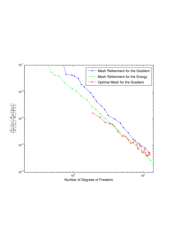
We show two relative errors against the number of degrees of
freedom. The first one is the error of the deformation
gradient in -norm over the -norm of the difference between the deformation gradient
of the atomistic solution and the homogeneous state, which is defined by
(6.1)
The second relative error is the absolute value of the energy
difference of the atomistic solution and the QC solution over the
absolute value of the energy change of the atomistic solution from the homogeneous state, which is defined by
(6.2)
Before we present the plots of the errors, we first introduce the mesh
generating schemes.
6.1. Mesh Construction
To avoid unnecessary technical difficulty in the mesh refinement
algorithm, we assume that the defect core is already captured in the middle of the chain. There are three mesh generating schemes we use.
The first mesh generating scheme is derived in
Section 7.1 of [6] using calculus of
variations. From this analysis, we get that the (quasi-)optimal mesh size in
the continuum region, with the restriction that the atomistic region is symmetric and has
atoms on each side, is given by
(6.3)
Since the mesh size can not change continuously and we restrict the
smallest mesh size in the continuum region to be , we use the
following algorithm to generate this mesh (we only list the case on the right hand side of the atomistic region):
Algorithm 1.
(1)
Set atom to be the middle of the atomistic region.
(2)
Choose so that there are atoms on each side of the
atomistic region.
(3)
Choose to be for every element on the right hand side
of the atomistic region until , where is the
distance between the right boundary of the previous element and the middle of the atomistic region.
(4)
Choose according to (6.3) until the right
boundary of the newly created element is out of the right limit of
the chain.
∎
The second mesh generating scheme is essentially a mesh refinement
process according to the error estimator with respect to the
deformation gradient according to Lemma 3.3,
Lemma 3.3 and Lemma 3.3. The mesh
refinement algorithm is stated as follows:
Algorithm 2.
(1)
Set atom to be the middle of the atomistic region.
(2)
Choose atoms on each side of the atomistic region.
(3)
Divide the left and the right part of the continuum region into
two equally large element
(4)
Compute the QC solution on this mesh and then compute the squared error indicator of each element and
sort these indicators according to its value.
(5)
Bisect the first sorted elements such that
(6.4)
where
is the error estimator of each element defined by
(6.5)
If the element is
near the atomistic region, merge the element into the atomistic region.
(6)
If the resulting mesh reaches the maximal number of degrees of
freedom, stop the process, else, go to Step 4.
∎
The third mesh generating scheme is the mesh refinement
process according to the error estimator with respect to the
energy which is defined by
(6.6)
for each element and the refinement algorithm is exactly the same.
In short, the first and second mesh generating schemes tend to
minimize the error in the deformation gradient and the third one tends
to minimize the error in the total energy.
6.2. Numerical Results
We compare the relative errors defined in
6.1 and 6.2. We plot
the relative errors against the number of degrees of freedom with
respect to the meshes generated.
Figure 1. Relative Error of the GradientFigure 2. Efficiency Factor of the Gradient
Figure 1 shows that the
pre-defined optimal mesh performs better than the two
mesh refinement strategies for a fix number of degrees of freedom. The
possible reason for this is that, due to some technical difficulty in
coding, both of the mesh refinement algorithms tend to produce larger atomistic
region by merging the elements in the continuum region to the atomistic region and create some unnecessary degrees of freedom. For the two mesh
refinement strategies, the one according to the gradient error indicator perform better asymptotically.
Figure 2 shows the efficiency
factor of the error estimator of the deformation gradient. It shows
that the efficiency factor is comparatively large but decreases as the
number of degrees of freedom increases and
finally become stable. The reason for this phenomenon lies in the form
of the external force. One can show that if the
external force takes the form of , where is
the distance to the centre of the defect, then the residual due to the
external force is of order as opposed to order in general
which is achieved by our analysis. As a result, our estimate
exaggerate the real error by for this particular
external force. This phenomenon gradually disappear as the continuum region moves apart from the centre of the defect since
the influence of this exaggeration is eliminated as the external force tends to when it is away from the centre of the defect, which
makes the residual of the sotred energy become the leading error term. It can also well explain the fact that the efficiency of
the estimate is better for the mesh refinement strategies than the
pre-defined mesh for a certain number of degrees of freedom, as the
two mesh refinement algorithms tend to put more atoms in the atomistic
region, i.e., the continuum region is further away from the centre of
defect than that of the pre-defined mesh.
Figure 3. Relative Error of the Total EnergyFigure 4. Efficiency Factor of the Energy
Figure 3 shows that the refinement
based on the energy error performs the best among all the three mesh generating schemes.
Figure 4 shows the efficiency
factor of the error estimator of the energy. For the same reason, this
factor decreases as the
number of degrees of freedom increases and finally becomes stable.
7. Conclusion
We have presented the a posteriori error estimates for the Consistent
Energy-Based QC method in one dimension. The procedure of the estimate
is the same as that in [8]. However, since the
formulation of the QC problem is newly developed and is totally
different from previous ones, new techniques have been developed and
applied to deal with the difficulty in the analysis. Several results
derived may be of independent interest and usefulness. In addition,
the error estimate of the total energy is also derived. Numerical
experiments are also implemented to illustrate our analysis.
Particular interesting future work are the extension and the
implementation of the a posteriori error estimate in higher
dimensional problems. The difficulty lies in the complication of the
formulation and the varied location of the
interaction bonds. However, since a priori analysis for the two
dimensional problem has been proposed
[6], ways of circumventing these difficulties could be
a source of reference.
Appendix A Detailed Analysis for the Residuals of the Stored Energy
In this section, we provide the omitted detailed analysis for the
residuals of the stored energy, namely
where , and .
The idea is to find the differences defined by
(A.1)
and
(A.2)
for each interaction bond .
We have analyzed the cases that and and are left with the analysis for the cases that is
across the atomistic-continuum interface and the boundaries of the
elements in the continuum region. There are three cases and in each
case there are three subcases to be considered.
Case 1: is across two adjacent elements . In this case and the atomistic
contribution of the interaction bond in the QC energy is .
Subcase 1: If , then , , , and
We have
and
(A.3)
Subcase 2: If , then , , , and
We have
and
(A.4)
Subcase 3: If , then , , , and
We have
and
(A.5)
Case 2: is across the left atomistic-continuum interface of an
atomistic region.
Subcase 1: If , then , ,
,
and
We have
(A.6)
and
(A.7)
Subcase 2: If ,
then , ,
,
and
We have
(A.8)
and
(A.9)
Subcase 3: If ,
then , ,
, , ,
and
We have
(A.10)
Case 2: is across the right atomistic-continuum interface of an
atomistic region.
Subcase 1: If , then , ,
,
and
We have
(A.11)
and
(A.12)
Subcase 2: If , then , ,
, , and
(A.13)
We have
(A.14)
and
(A.15)
Subcase 3: If , then , ,
, , and
(A.16)
We have
(A.17)
and
(A.18)
Appendix B Approximation Properties
In this section, we prove some approximation properties which we have
used but are hardly found in standard text books.
Lemma 11.
Let be a periodic function with
being one of its period. Let be a interpolation of
with respect to the nodes in , subject
to a constant, i.e., , for , and is extended periodically with period . Then the
following estimate holds:
(B.1)
where and denote the weak derivatives of and respectively.
Proof.
First we note that, since and is a
interpolation of ,
the weak derivative of on is defined by
Since is piecewise differentiable, we have
where is the weak derivative of .
By the periodicity of and , and Cauchy-Schwarz Inequality, we have
Taking the square root on both sides gives the stated result.
∎
Lemma 12.
Let and is the
function that interpolates at the points and . We have the
following inequality:
(B.2)
Proof.
Since and , by the definition of , we have
and equivalently,
where denotes the weak derivative of on . This shows
that is the best approximation of in
the space of functions as is a constant. Therefore, by the
property of best approximation,
(B.3)
for any constant . In particular, if we choose to be , the
stated result holds.
∎
Appendix C Discrete Sobolev Inequalities on Non-uniform mesh
In this section, we prove some discrete Soblev inequalities on
non-uniform mesh that are used in the residual analysis for the
external force. These results are extensions to the inequalities proved in
[7, Lemma A.1, Lemma A.2, Theorem A.4] on non uniform
mesh.
Lemma 13.
Let , and , , . If , then
(C.1)
where, , for and for .
Proof.
Let , then
Since
we have
Divide both sides by , we obtain the stated result.
∎
Lemma 14.
(Discrete Poincare’s Inequality) Suppose that , with , .
Let such that and such that . Define to be the set and to be the set ,
then
Put these results together, we obtain the stated result for .
For ,
The stated result is obtained by taking the maximum of and over and .
∎
Lemma 15.
(Discrete Friedrichs’ Inequality) Suppose that , , ,
, are the same as in Lemma C. Let
such that , and such that , then
(C.3)
for .
Proof.
For ,
For ,
and
Thus we have
∎
Remark 2. The bounds we have got here are not optimal as if ’s and
’s vary too much, taking the maximum of them in the
inequalities could significantly reduce the sharpness of the estimate. However, for the
analysis of this paper, such a bound is optimal enough to produce
efficient error estimators and we leave the work of looking for optimal
bounds to future work.
∎
Theorem 16.
(bounds on the interpolation error) Let , ,
with . Let
and such that and
(C.4)
where . Define such that and such that , and and are defined
in the same way. Let , be the same sets defined in Lellmma C and
be the set . Then, for ,
as . Since , from which we know
, the stated estimate holds.
∎
References
[1]
Marcel Arndt and Mitchell Luskin.
Goal-oriented atomistic-continuum adaptivity for the quasicontinuum
approximation.
Int. J. Multiscale Comput. Engrg., 5(49-50):407–415, 2007.
[2]
Marcel Arndt and Mitchell Luskin.
Error estimation and atomistic-continuum adaptivity for the
quasicontinuum approximation of a Frenkel-Kontorova model.
Multiscale Model. Simul., 7(1):147–170, 2008.
[3]
Marcel Arndt and Mitchell Luskin.
Goal-oriented adaptive mesh refinement for the quasicontinuum
approximation of a Frenkel-Kontorova model.
Comput. Methods Appl. Mech. Engrg., 197(49-50):4298–4306,
2008.
[4]
W. E and P. Ming.
Analysis of the local quasicontinuum method.
In Frontiers and prospects of contemporary applied mathematics,
volume 6 of Ser. Contemp. Appl. Math. CAM, pages 18–32. Higher Ed.
Press, Beijing, 2005.
[5]
P. Lin.
Theoretical and numerical analysis for the quasi-continuum
approximation of a material particle model.
Math. Comp., 72(242):657–675, 2003.
[6]
C. Ortner and A.V. Shapeev.
A priori error analysis of an energy-based atomistic/continuum
coupling method for pair interactions in two dimensions.
arXiv:1104.0311v1.
[7]
C. Ortner and E. Süli.
Analysis of a quasicontinuum method in one dimension.
M2AN Math. Model. Numer. Anal., 42(1):57–91, 2008.
[8]
C. Ortner and H. WANG.
A priori error estimates for energy-based quasicontinuum
approximations of a periodic chain.
2010.
to appear in M3AS Math. Model. Meth. Appl. Sci.
[9]
Serge. Prudhomme, Paul. Bauman, and Tinsley Oden.
Error control for molecular statics problems.
Int. J. Multiscale Comput. Engrg., 4:647–662, 2007.
[10]
A.V. Shapeev.
Consistent energy-based coupling of atomistic and continuum static
models for two-body potential.
arXiv:1010.0512.
[11]
T. Shimokawa, J.J. Mortensen, J. Schiotz, and K.W. Jacobsen.
Matching conditions in the quasicontinuum method: Removal of the
error introduced at the interface between the coarse-grained and fully
atomistic region.
Phys. Rev. B, 69(21):214104, 2004.