The $p_{x}+ip_{y}$ Chiral Superconductor wire weakly coupled to two metallic rings pierced by an external flux

Abstract

We consider a p-wave superconductor wire coupled to two metallic rings. confined to a one-dimensional wire. At the two interface between the the wire and the metallic rings the pairing order parameter vanishes, as result two zero modes Majorana fermion appear. The two metallic rings are pierced by external magnetic fluxes. The special features of the Majorana Fermions can be deduced from the correlation between the currents in the two rings.

I Introduction

Topological Superconductors are characterized by the invariance under charge conjugation symmetry. As a result of this invariance zero modes Majorana fermion appear at the interfaces between the superconductor a metal. $Sr_{2}Ru$ is the material where Majorana fermion might be observed since the pairing order parameter is characterized by $p_{x}+ip_{y}$ symmetry. The electronic excitations for the ground state pairing $p_{x}+ip_{y}$ are given by half vortices which are zero mode Majorana fermions Kitaev ; DunghaiLee ; Oreg1 ; Oreg2 .

The realization of the p-wave superconductors physics and the formation of the zero mode Majorana Fermions at the edges of the wire can be achieved using a p-wave wire of length $L$ coupled to two metallic rings which are pierced by external magnetic fields.The current in the rings is coupled to the p-wave wire trough the Majorana modes which are bound at the interface. For different fluxes in the rings we find that the excitations in the wires become imaginary resulting in an unstable vanishing current. The only stable current are obtained for the case that the imaginary part vanishes. The stable current are obtained for special relations between the magnetic fluxes and the wire excitations energy. This feature is attributed to the existence of the Majorana fermions. We find that the correlation between the currents in the two rings is affected by the presence of the Majorana Fermions. Therefore the model introduced here can be used for the identification of the Majorana fermions.

The content of this paper is as follows: In chapter $II$ we present the model of the the $p-wave$ wire coupled to two metallic rings. Using the left and right mover we obtain the continuum representation of the superconductor wire. At the two edges of the wire we obtain the two zero modes of the wire. The effect of the coupling between the wire and the metallic rings is dominated by the zero modes of the wire. As a result we derive the effective Hamiltonian between the zero modes and the metallic rings. This effective Hamiltonian is controlled by the low energy excitation in the wire (the coupling energy between the two edges) $\epsilon\approx|\Delta_{0}|e^{-L|\Delta_{0}|}$ ,$L|\Delta_{0}|>>1$ where $\Delta_{0}$ is the pairing field and $L$ is the length of the wire. In section $III$ we consider the case that the wire energy $\epsilon\rightarrow 0$. In section $IV$ we consider the case where the wire energy is finite. Section $V$ is devoted to conclusions.

II- The model for the p-wave wire weakly coupled to two rings pierced by external fluxes

The p-wave wire of length $L$ is given by the Hamiltonian $H_{P-W}$ :

$$H_{P-W}=-t\sum_{x,x^{\prime}}(C^{+}(x)C(x^{\prime})+h.c.)-\mu_{F}\sum_{x}C^{+}(x)C(x)-\hat{\Delta}\sum_{x,x^{\prime}}[\gamma_{x,x^{\prime}}C^{+}(x)C^{+}(x^{\prime})+\gamma_{x,x^{\prime}}C(x^{\prime})C(x)]$$ (1)

The pairing gap is given by $\hat{\Delta}$ and the polarized fermion operator is given by $C(x)\equiv C_{\sigma=\uparrow}(x)$. The matrix elements $\gamma_{x,x^{\prime}}$ obey obey the p-wave symmetry: $\gamma_{x,x^{\prime}=x-a}=-\gamma_{x,x^{\prime}=x+a}$, $|\gamma_{x,x^{\prime}}|=1$, therefore the time reversal and parity symmetry are both broken and obeys the pairing boundary conditions $\hat{\Delta}(x=0)=\hat{\Delta}(x=L)=0$ and $\hat{\Delta}(x)=\hat{\Delta}_{0}$ for $0<x<L$.

We introduce the right and left fermions in the continuum representation for the fermions in the wire : $C(x=na)\sqrt{a}\rightarrow C(x)=e^{ik_{F}x}\hat{C}_{R}(x)+e^{-ik_{F}x}\hat{C}_{L}(x)$ and find that equation $1$ is replaced by the Hamiltonian :

$$H_{P-W}=\int dx[v_{F}\Psi^{\dagger}(x)\sigma^{z}(-i\partial_{x})\Psi(x)+\Delta(x)\Psi^{\dagger}(x)\sigma^{x}\Psi(x)]$$ (2)

This Hamiltonian is invariant under the charge conjugation symmetry. The spinor $\Psi^{\dagger}(x)=[C^{\dagger}_{R}(x),C_{L}(x)]\equiv[e^{\frac{i\pi}{4}}\hat{C}^{\dagger}_{R}(x),e^{\frac{-i\pi}{4}}\hat{C}_{L}(x)]$ satisfies the reality constraint condition $K\Psi^{\dagger}(x)=\Psi(x)$, where $K$ is the charge conjugation operator.

The pairing field $\Delta(x)\equiv 4\hat{\Delta}(x)\sin(k_{F}a)$ can be written as $\Delta(x)=M_{L}(x)+M_{R}(x-L)$ where $M_{L}(x)=\frac{\Delta(0)}{2}sgn(x)$ and $M_{R}(x-L)=\frac{\Delta(0)}{2}sgn(x-L)$ obeys the domain wall property: $M_{L}(-x)=-M_{L}(x)$ (at x=0) , $M_{R}(-(x-L))=-M_{R}(x-L)$ (at x=L) . The zero modes eigenfunctions are given by $\eta_{\lambda}(x)=[\eta_{1}(x),\eta_{2}(x)]^{T}$ and eigenstates of the operator $\sigma^{y}\eta_{\lambda}(x)=\lambda\eta_{\lambda}(x)$ with $\lambda=\pm 1$. The zero mode spinor which is localized around $x=0$ is identified with $\lambda=-1$ and the second one which localized around $x=L$ is identified with $\lambda=1$

$$\eta_{Left}(x)\equiv\eta_{\lambda=-1}(x)=e^{\frac{-1}{v_{F}}\int_{0}^{x}\Delta(x^{\prime})\,dx^{\prime}}\frac{e^{i\frac{\pi}{4}}}{\sqrt{2}}[1,-i]^{T}$$

$$\eta_{Right}(x)\equiv\eta_{\lambda=1}(x)=e^{\frac{1}{v_{F}}\int_{L}^{x}\Delta(x^{\prime})\,dx^{\prime}}\frac{e^{-i\frac{\pi}{4}}}{\sqrt{2}}[1,i]^{T}$$

The spinor operator $\Psi(x)$ with the two zero mode Majorana operators $\alpha_{l}$ (at the left edge) and $\alpha_{r}$ (at the right edge), $(\alpha_{r})^{2}=(\alpha_{l})^{2}=\frac{1}{2}$ takes the form :

$$\Psi(x)\rightarrow\Psi(x)+\alpha_{r}\eta_{\lambda=1}(x)+\alpha_{l}\eta_{\lambda=-1}(x)$$ (4)

As a result the low energy of the p-wave wire is given by:

$$H_{P-W}=\int dx[v_{F}\Psi^{\dagger}(x)\sigma^{z}(-i\partial_{x})\Psi(x)+\Delta(x)\Psi^{\dagger}(x)\sigma^{x}\Psi(x)]\approx\frac{i}{2}\epsilon\alpha_{l}\alpha_{r}$$ (5)

where $\epsilon\approx|\Delta_{0}|e^{-L|\Delta_{0}|}$ ,$L|\Delta_{0}|>>1$.

At this stage we include the two rings Hamiltonian pierced by the fluxes $\hat{\varphi}_{i}$ , $i=1,2$ and length $l_{ring}<<L$. The left ring is restricted to the region $-l_{ring}\leq x\leq 0$ and the right ring is restricted to $L\leq x\leq L+l_{ring}$. Since only the wire fields at $x=0$ and $x=L$ are involved we fold the space of the right ring $i=2$ such that both rings are restricted to the region $-l_{ring}\leq x\leq 0$. As a result the external fluxes obey: $\hat{\varphi}_{1}\rightarrow\hat{\varphi}_{1}$ and $\hat{\varphi}_{2}\rightarrow-\hat{\varphi}_{2}$. In addition we replace for each ring the fermion operator $\psi_{i}(x)$,i=1,2 by the $right$ $R_{i}(x)$ and $left$ fermions $L_{i}(x)$:

$$\psi_{i}(x)=R_{i}(x)e^{ik_{F}x}+L_{i}(x)e^{-ik_{F}x}$$ (6)

We replace for each ring the $right$ and $left$ movers by four Mayorana operators:

$$r_{i}\equiv(R_{i}(0)-R^{\dagger}_{i}(0))(-i)$$

$$l_{i}\equiv L_{i}(0)+L^{\dagger}_{i}(0)$$

The the matrix element between the wire and rings is given by $-g$. As a result the low energy hopping Hamiltonian is given by:

$$H_{T}=\frac{-ig}{\sqrt{2}}[\alpha_{l}(r_{1}+l_{1})+\alpha_{r}(r_{2}-l_{2})]$$ (8)

We replace the Majorana zero modes $\alpha_{l}$ and $\alpha_{r}$ by the fermion pair, $q=\alpha_{l}+i\alpha_{r}$, $q^{\dagger}=\alpha_{l}-i\alpha_{r}$ which obey: $[q,q^{\dagger}]_{+}=1$, $q^{\dagger}|0>=|1>$ and $q|1>=|0>$ where $|0>$ is ground state of wire and rings: $R_{i,p}(x)|0>=L_{i,p}(x)|0>=R^{\dagger}_{i,h}(x)|0>=L^{\dagger}_{i,h}(x)|0>=q|0>=0$. Where $R_{i,p}(x)$, $L_{i,p}(x)$ are the particle operators and $R^{\dagger}_{i,h}(x)$, $L^{\dagger}_{i,h}(x)$ are the holes operators $R^{\dagger}_{i,h}(x)$, $L^{\dagger}_{i,h}(x)$. The right and left mover are given as a linear combination of particles and holes operators. $R_{i,p}(x)$ $L_{i,p}(x)$ represent the annihilation of particles and $R^{\dagger}_{i,h}(x)$, $L^{\dagger}_{i,h}(x)$ are the creation operators for holes.

$$R_{i}(x)=R_{i,p}(x)+R^{\dagger}_{i,h}(x);\hskip 7.22743ptL_{i}(x)=L_{i,p}(x)+L^{\dagger}_{i,h}(x)$$ (9)

Using the Fermionic representation we replace $H_{P-W}$ given in equation $5$ and $H_{T}$ given in equation $(8)$ by :

$$H_{P-W}+H_{T}\equiv\epsilon q^{\dagger}q-\frac{ig}{2\sqrt{2}}[(q+q^{\dagger})(r_{1}+l_{1})-i(q-q^{\dagger})(r_{2}-l_{2})]$$ (10)

The value of the wire energy $\epsilon$ in equations $5,10$ is based on the projection of the spinor (in equation $4$) on the zero modes $\eta_{\lambda=1}(x)$ and $\eta_{\lambda=-1}(x)$. Since the leads couple to the modes in the wire, we expect that the non-zero modes will give rise to a finite width of the energy $\epsilon$. Therefore for finite energies we will replace $\epsilon$ by $\hat{\epsilon}\equiv\epsilon-i\Gamma$, where the width $\Gamma\propto g^{4}$.

We perform an exact integration over the fermion operators $q$,$q^{\dagger}$ and find the time dependent effective interaction $H_{eff}(t)$:

$$H_{eff}(t)=\frac{-ig^{2}}{2}\int\,dt^{\prime}\mu[t,t^{\prime}]e^{-i\frac{\hat{\epsilon}}{\hbar}(t-t^{\prime})}[r_{2}(t)-l_{2}(t)+i(r_{1}(t)+l_{1}(t))][r_{2}(t^{\prime})-l_{2}(t^{\prime})-i(r_{1}(t^{\prime})+l_{1}(t^{\prime}))]$$

where $\mu[t,t^{\prime}]$ is the step function which is one for $t>t^{\prime}$.

III-The effective interaction $H_{eff}(t)$ in the limit $\epsilon\rightarrow 0$

When $\epsilon\rightarrow 0$ equation $11$ is replaced by :

$$H_{eff}(t)=\frac{-ig^{2}}{2}\int\,dt^{\prime}\mu[t,t^{\prime}][r_{2}(t)-l_{2}(t)+i(r_{1}(t))+l_{1}(t)][r_{2}(t^{\prime})-l_{2}(t^{\prime})-i(r_{1}(t^{\prime})+l_{1}(t^{\prime})]$$

Using the scaling analysis given in davidimpurity we observe that the effective interaction flows to the strong coupling limit and find $g^{2}(b)=g^{2}b^{2-\alpha}$, $\alpha\approx 1$ where $b>1$. Since the coupling constant $g(b)$ flows to infinity, the only way a solution will exists if the effective interaction annihilates the ground state: $H_{eff}(t)|0>=0$. Therefore the physical solution is given by the $constraint$ rings equation:

$$[r_{2}(t)-l_{2}(t)-i(r_{1}(t)+l_{1}(t)]|0>=0$$ (13)

Since $R_{i,p}(x)|0>=L_{i,p}(x)|0>=R^{\dagger}_{i,h}(x)|0>=L^{\dagger}_{i,h}(x)|0>=0$ the constraint condition implies for particles ($p$ stands for particles) the equation : $[i(R^{\dagger}_{2,p}-L^{\dagger}_{1,p})-(L^{\dagger}_{2,p}-R^{\dagger}_{1,p})]|0>=0$; and for holes ($h$ stands for holes) $[i(R_{2,h}-L_{1,h})-(L_{2,h}-R_{1,h})]|0>=0$. We find the constraint equation:

$$\psi_{1}(x=0)\equiv R_{1}(x=0)+L_{1}(x=0)=e^{-i\frac{\pi}{2}}[R_{2}(x=0)+L_{2}(x=0)]\equiv e^{-i\frac{\pi}{2}}\psi_{2}(x=0)=\widetilde{\psi}_{2}(x=0)$$ (14)

The explicit identity contains the phase factor $e^{-i\frac{\pi}{2}}$ which is obtained from Bosonization (see below). Following equation $14$ we find the constraint condition for the ground state $|0>$:

$$\kappa\equiv[\psi_{1}(x)-\psi_{2}(x)]|_{x=0},\hskip 14.45377pt\kappa|0>=0$$ (15)

Following rings we find two additional constraints equation :

$$\mathcal{E}\equiv[(-i\partial_{x}-\frac{2\pi}{l_{ring}}\hat{\varphi}_{1})^{2}\psi_{1}(x)-(-i\partial_{x}+\frac{2\pi}{l_{ring}}\hat{\varphi}_{2})^{2}\psi_{2}(x)]|_{x=0},\hskip 14.45377pt\mathcal{E}|0>=0$$ (16)

$$\mathcal{J}\equiv[(-i\partial_{x}-\frac{2\pi}{l_{ring}}\hat{\varphi}_{1})\psi_{1}(x)+(-i\partial_{x}+\frac{2\pi}{l_{ring}}\hat{\varphi}_{2})\psi_{2}(x)]|_{x=0},\hskip 14.45377pt\mathcal{J}|0>=0$$ (17)

Any eigenstate of N particles must satisfy the set of equations $15-17$ with the periodic boundary condition $\psi_{i}(x)=\psi_{i}(x+l_{ring})$. For the case $N=1$ (one particle) we have :

$$|N=1>=\int_{-l_{ring}}^{0}\,dx[f_{1}(x)\psi^{\dagger}_{i}(x)+f_{2}(x)\psi^{\dagger}_{2}(x)]$$ (18)

where $f_{i}(x)$ are the amplitudes . Using equations $15-17$ we find finite solutions for the amplitudes $f_{i}(x)$ only when the fluxes are equal.

IV-The finite limit $\epsilon\neq 0$

In order to study the finite limit $\epsilon\neq 0$ we will use the zero mode Bosonization method davidimpurity ; Berkovits . The right $R_{i}(x)$ and left $L_{i}(x)$ fermions for each ring $i=1,2$ is given by:

$$R_{i}(x)=\sqrt{\frac{\Lambda}{2\pi}}Z_{i}e^{i\alpha_{R,i}}e^{\frac{2\pi}{l_{ring}}(N_{R,i}-\frac{1}{2})x}e^{i\sqrt{4\pi}\vartheta_{R,i}(x)}$$

$$L_{i}(x)=\sqrt{\frac{\Lambda}{2\pi}}Z_{i}e^{i\alpha_{L,i}}e^{\frac{2\pi}{l_{ring}}(N_{L,i}-\frac{1}{2})x}e^{i\sqrt{4\pi}\vartheta_{L,i}(x)}$$

Where $Z_{1}Z_{2}=-Z_{2}Z_{1}$ are Majorana variable which ensure the anti-commutation between the two rings in the bosonic representation. In the bosonic representation we have the zero modes $\alpha_{R,i}$ $\alpha_{L,i}$ bosons and their conjugates ,$N_{R,j}$,$N_{L,j}$. The zero modes obey the commutation rules :$[-\alpha_{L,i},N_{L,j}]=i\delta_{i,j}$ and $[\alpha_{R,i},N_{R,j}]=i\delta_{i,j}$.

As a result we obtain the zero mode representation in terms of the fermion numbers $N_{L,i}$,$N_{R,i}$ and fluxes $\hat{\varphi}_{i}$ in each ring:

$$H_{0}=\frac{\pi v_{F}\hbar}{2l_{ring}}[(N_{L,1}-N_{R,1}+2\hat{\varphi}_{1})^{2}+(N_{L,1}+N_{R,1})^{2}]+\frac{\pi v_{F}\hbar}{2l_{ring}}[(N_{L,2}-N_{R,2}+2\hat{\varphi}_{2})^{2}+(N_{L,1}+N_{R,1})^{2}]$$

Using the equations of motion $i\hbar\frac{d\alpha_{R,i}}{dt}=[\alpha_{R,i},H_{0}]$ and $i\hbar\frac{d\alpha_{L,i}}{dt}=[\alpha_{L,i},H_{0}]$ ,$i=1,2$ we obtain the zero mode representation in the interaction picture. We will use the zero mode representation $\alpha^{I}_{R,i}(t)$, $\alpha^{I}_{L,i}(t)$ in the interaction picture in order to evaluate equation $15$. We find that $H_{eff}(t)$ is given in terms of the zero mode functions $F(t+\frac{\tau}{2})$ and $G(t-\frac{\tau}{2})$ :

$$H_{eff}(t)=-2i\hat{g}^{2}\int_{0}^{\infty}\,d\tau F(t+\frac{\tau}{2})e^{-i\frac{\hat{\epsilon}}{\hbar}\tau}G(t-\frac{\tau}{2})$$ (21)

where $\hat{g}^{2}=g^{2}\frac{\Lambda}{2\pi}$ is the coupling constant and $\nu_{0}\equiv\frac{\epsilon}{\hbar}$, $\nu_{i}\equiv\frac{2\pi v_{F}}{l_{ring}}\hat{\varphi}_{i}$ are the equivalent wire and rings frequencies and $\hat{\Gamma}=\frac{\Gamma}{\hbar}$ is the width. The functions $F(t+\frac{\tau}{2})$ and $G(t-\frac{\tau}{2})$ are given by:

$$F(t+\frac{\tau}{2})=Z_{2}((\sin\alpha^{I}_{R,2}(t+\frac{\tau}{2})-\cos\alpha^{I}_{L,2}(t+\frac{\tau}{2}))+iZ_{1}((\sin\alpha^{I}_{R,1}(t+\frac{\tau}{2})-\cos\alpha^{I}_{L,1}(t+\frac{\tau}{2}))=$$

$$Z_{2}[\sin\alpha^{I}_{R,2}(t)\cos(\nu_{2}\tau)+\cos\alpha^{I}_{R,2}(t)\sin(\nu_{2}\tau)-\cos\alpha^{I}_{L,2}(t)\cos(\nu_{2}\tau)+\sin\alpha^{I}_{L,2}(t)\sin(\nu_{2}\tau)]$$

$$+iZ_{1}[\sin\alpha^{I}_{R,1}(t)\cos(\nu_{1}\tau)-\cos\alpha^{I}_{R,1}(t)\sin(\nu_{1}\tau)+\cos\alpha^{I}_{L,1}(t)\cos(\nu_{1}\tau)-\sin\alpha^{I}_{L,1}(t)\sin(\nu_{1}\tau)]$$

$$G(t-\frac{\tau}{2})=Z_{2}((\sin\alpha^{I}_{R,2}(t-\frac{\tau}{2})-\cos\alpha^{I}_{L,2}(t-\frac{\tau}{2}))-iZ_{1}((\sin\alpha^{I}_{R,1}(t-\frac{\tau}{2})+\cos\alpha^{I}_{L,1}(t-\frac{\tau}{2}))=$$

$$Z_{2}[\sin\alpha^{I}_{R,2}(t)\cos(\nu_{2}\tau)-\cos\alpha^{I}_{R,2}(t)\sin(\nu_{2}\tau)-\cos\alpha^{I}_{L,2}(t)\cos(\nu_{2}\tau)-\sin\alpha^{I}_{L,2}(t)\sin(\nu_{2}\tau)]$$

$$-iZ_{1}[\sin\alpha^{I}_{R,1}(t)\cos(\nu_{1}\tau)+\cos\alpha^{I}_{R,1}(t)\sin(\nu_{1}\tau)+\cos\alpha^{I}_{L,1}(t)\cos(\nu_{1}\tau)-\sin\alpha^{I}_{L,1}(t)\sin(\nu_{1}\tau)]$$

We perform the integration with respect $\tau$ and find:

$$H_{eff}\approx H^{real}_{eff}+iH^{Im.}_{eff}$$ (24)

where $H^{real}_{eff}$ is the real part of the effective action:

$$H^{real}_{eff}=$$

$$\frac{\hbar\hat{g}^{2}\nu_{0}}{\nu_{0}^{2}+\hat{\Gamma}^{2}}[\cos(2\alpha_{R,2})-\cos(2\alpha_{L,2})-\cos(2\alpha_{L,1})+\cos(2\alpha_{R,1})+2(\sin(\alpha_{R,2}+\alpha_{L,2})-\sin(\alpha_{R,1}+\alpha_{L,1}))]$$

$$-2\hbar\hat{g}^{2}(\frac{\nu_{0}-\nu_{1}}{(\nu_{0}-\nu_{1})^{2}+\hat{\Gamma}^{2}}+\frac{\nu_{0}+\nu_{1}}{(\nu_{0}+\nu_{1})^{2}+\hat{\Gamma}^{2}})[1+\sin(\alpha_{R,1}-\alpha_{L,1})]$$

$$-2\hbar\hat{g}^{2}(\frac{\nu_{0}-\nu_{2}}{(\nu_{0}-\nu_{2})^{2}+\hat{\Gamma}^{2}}+\frac{\nu_{0}+\nu_{2}}{(\nu_{0}+\nu_{2})^{2}+\hat{\Gamma}^{2}})[1+\sin(\alpha_{R,2}-\alpha_{L,2})]$$

The imaginary part $H^{Im.}_{eff}$ of the action causes the current to vanish. Finite solutions will be obtained for the ground states $|0>$ which obey $H^{Im.}_{eff}|0>=0$. Therefore the solutions for finite currents are equivalent to a constraint condition for the ground state $|0>$.

$$H^{Im.}_{eff}=Z_{2}Z_{1}\hat{g}^{2}[\frac{\hat{\Gamma}}{(\nu_{0}-\frac{\nu_{2}-\nu_{1}}{2})^{2}+\hat{\Gamma}^{2}}+\frac{\hat{\Gamma}}{(\nu_{0}+\frac{\nu_{2}-\nu_{1}}{2})^{2}+\hat{\Gamma}^{2}}]$$

$$[(\sin(\alpha_{R,2})-\cos(\alpha_{L,2}))(\cos(\alpha_{L,1})+\sin(\alpha_{R,1}))+(\sin(\alpha_{R,2})+\sin(\alpha_{L,2}))$$

$$(\cos(\alpha_{R,1})+\sin(\alpha_{L,1}))]$$

$$+Z_{2}Z_{1}\hat{g}^{2}[\frac{\hat{\Gamma}}{(\nu_{0}-\frac{\nu_{2}+\nu_{1}}{2})^{2}+\hat{\Gamma}^{2}}+\frac{\hat{\Gamma}}{(\nu_{0}+\frac{\nu_{2}+\nu_{1}}{2})^{2}+\hat{\Gamma}^{2}}]$$

$$[(\sin(\alpha_{R,2})-\cos(\alpha_{L,2}))(\cos(\alpha_{L,1})+\sin(\alpha_{R,1}))-(\cos(\alpha_{R,2})+\sin(\alpha_{L,2}))$$

$$(\cos(\alpha_{R,1})-\sin(\alpha_{L,1}))]$$

We find two cases for which a finite solution exist.

The first case corresponds to $\nu_{0}\approx(|\frac{\nu_{2}-\nu_{1}}{2}|)$ with the solution:

$$H^{Im.}_{eff}|0>=0$$

$$\alpha_{R,2}=\alpha_{R,1}+u$$

$$\alpha_{L,2}=\alpha_{L,1}-u$$

The second case corresponds to $\nu_{0}\approx(\frac{\nu_{2}+\nu_{1}}{2})$ with the solution:

$$H^{Im.}_{eff}|0>=0$$

$$\alpha_{R,2}=-\alpha_{R,1}+u$$

$$\alpha_{L,2}=-\alpha_{L,1}-u$$

We introduce the definitions for the zero mode fields :

$$\alpha_{1}=\alpha_{2}\equiv\alpha;\hskip 14.45377pt\beta_{2}=\beta_{1}-2u,\beta_{1}\equiv\beta$$ (29)

The solutions are independent on the arbitrary field $u$ which plays the role of a gauge condition and has to be integrated out. We integrated over the field $u$ we find the effective Hamiltonian for the conditions $\nu_{0}\approx(\frac{\nu_{2}-\nu_{1}}{2})$ and $\nu_{0}\approx(\frac{\nu_{2}+\nu_{1}}{2})$. We introduce the magnetic flux the variables $\bar{\varphi}$ and $\Delta$:

$$\bar{\varphi}=\frac{\hat{\varphi}_{1}+\hat{\varphi}_{2}}{2};\Delta=\frac{\hat{\varphi}_{1}-\hat{\varphi}_{2}}{2}$$ (30)

We can write both cases in a closed form:

$$\frac{H}{\hbar}\approx\frac{\pi v_{F}}{2l_{ring}}[(-i\frac{d}{d\alpha}+2\hat{\varphi}_{1})^{2}+(-i\frac{d}{d\beta})^{2}]+\frac{\pi v_{F}}{2l_{ring}}[(-i\frac{d}{d\alpha}+2\hat{\varphi}_{2})^{2}+(-i\frac{d}{d\beta})^{2}]+$$

$$[\frac{2\hat{g}^{2}\nu_{0}}{\nu_{0}^{2}+\hat{\Gamma}^{2}}\sin(\alpha)\sin(\beta)-2\hat{g}^{2}[\frac{\nu_{0}-(\bar{\varphi}+\Delta)}{(\nu_{0}-(\bar{\varphi}+\Delta)^{2}+\hat{\Gamma}^{2}}+\frac{\nu_{0}+(\bar{\varphi}+\Delta)}{(\nu_{0}+(\bar{\varphi}+\Delta)^{2}+\hat{\Gamma}^{2}}]\sin(\beta)$$

$$-2\hat{g}^{2}[\frac{\nu_{0}-(\bar{\varphi}+\Delta)}{(\nu_{0}-(\bar{\varphi}+\Delta)^{2}+\hat{\Gamma}^{2}}+\frac{\nu_{0}+(\bar{\varphi}+\Delta)}{(\nu_{0}+(\bar{\varphi}+\Delta)^{2}+\hat{\Gamma}^{2}}+\frac{\nu_{0}-(\bar{\varphi}-\Delta)}{(\nu_{0}-(\bar{\varphi}-\Delta)^{2}+\hat{\Gamma}^{2}}+\frac{\nu_{0}+(\bar{\varphi}-\Delta)}{(\nu_{0}+(\bar{\varphi}-\Delta)^{2}+\hat{\Gamma}^{2}}]]$$

$$(\delta_{\frac{\hat{\varphi}_{1}-\hat{\varphi}_{2}}{2},\nu_{0}}+\delta_{\frac{\hat{\varphi}_{1}+\hat{\varphi}_{2}}{2},\nu_{0}})$$

The first line of equation $31$ represents the the Hamiltonian for the two metallic rings pierced by the external fluxes expressed in therms of the zero mode of the metallic rings. The second part of equation $31$ represents the coupling between the wire and the two rings. We observe that this part is restricted by the constraint condition $\frac{\hat{\varphi}_{1}-\hat{\varphi}_{2}}{2}=\nu_{0}$ or $\frac{\hat{\varphi}_{1}+\hat{\varphi}_{2}}{2}=\nu_{0}$. This constraints represents the effect of the Majorana fermions on the p-wave wire.

In order two investigate the Hamiltonian in equation $31$ we will use the algebra of the zero modes david ; davidDirac ; Berkovits :

$$\hat{J}=N_{R}-N_{L}\equiv-2i\frac{d}{d\alpha};\hskip 14.45377pt\hat{Q}=N_{R}+N_{L}\equiv-2i\frac{d}{d\beta}$$ (32)

with the eigenvalues and commutation rules:

$$\hat{J}|J,Q>=J|J,Q>;J=0,\pm 1,\pm 2,..$$

$$\hat{Q}|J,Q>=Q|J,Q>;Q=0,\pm 1,\pm 2,..$$

From the commutation relations $[\alpha,\hat{J}]=2i$, $[\beta,\hat{Q}]=2i$ we establish the relations :

$$e^{i\alpha}|J,Q>=|J+1,Q>;e^{-i\alpha}|J,Q>=|J-1,Q>$$

$$e^{i\beta}|J,Q>=|J,Q+1>;e^{-i\beta}|J,Q>=|J,Q-1>$$

The eigenfunctions are given by:

$$<\alpha|J,Q=0>=\frac{1}{\sqrt{4\pi}}e^{i\alpha J};<\beta|J=0,Q>=\frac{1}{\sqrt{4\pi}}e^{i\alpha J}$$

Using the algebra of the zero modes we compute to lowest order (in perturbation theory) the energy for the ground state of the two rings coupled to the wire. As a function of the coupling constant $\lambda\equiv\frac{2\hat{g}^{2}}{\nu_{max}}<1$ and maximum frequency $\nu_{max}$ which is given by the electronic bandwidth frequency. We find for the ground state energy $E(\hat{\varphi}_{1},\hat{\varphi}_{2})$:

$$E(\hat{\varphi}_{1},\hat{\varphi}_{2})=[\frac{2\hbar\pi v_{F}}{l_{ring}}((\bar{\varphi}+\Delta)^{2}+(\bar{\varphi}-\Delta)^{2})$$

$$-\lambda(\frac{\nu_{max}}{\nu_{0}})(\frac{\nu_{0}-(\bar{\varphi}+\Delta)}{(\nu_{0}-(\bar{\varphi}+\Delta)^{2}+\hat{\Gamma}^{2}}+\frac{\nu_{0}+(\bar{\varphi}+\Delta)}{(\nu_{0}+(\bar{\varphi}+\Delta)^{2}+\hat{\Gamma}^{2}}+$$

$$\frac{\nu_{0}-(\bar{\varphi}-\Delta)}{(\nu_{0}-(\bar{\varphi}-\Delta)^{2}+\hat{\Gamma}^{2}}+\frac{\nu_{0}+(\bar{\varphi}-\Delta)}{(\nu_{0}+(\bar{\varphi}-\Delta)^{2}+\hat{\Gamma}^{2}})](\delta_{\nu_{0},\bar{\varphi}}+\delta_{\nu_{0},\Delta})$$

Using eq.36 we compute the currents $I_{i}=\frac{\partial E(\hat{\varphi}_{1},\hat{\varphi}_{2})}{\partial\hat{\varphi}_{i}}$ for the two rings $i=1,2$ using the conditions: $\nu_{0}\approx\frac{\hat{\varphi}_{1}-\hat{\varphi}_{2}}{2}\equiv\Delta$.

The current in ring one $I_{1}$ and ring two $I_{2}$ are represented in terms of $\bar{\varphi}=\frac{\hat{\varphi}_{1}+\hat{\varphi}_{2}}{2}$, $\nu_{0}=\Delta$ and the current amplitude $I_{0}=\frac{2\pi v_{F}}{l_{ring}}$

$$\frac{I_{1}}{I_{0}}=\bar{\varphi}+\nu_{0}-\lambda[\frac{\bar{\varphi}^{2}-\hat{\Gamma}^{2}}{(\bar{\varphi}^{2}+\hat{\Gamma}^{2})^{2}}+\frac{-(2\nu_{0}+\bar{\varphi})^{2}+\hat{\Gamma}^{2}}{(2\nu_{0}+\bar{\varphi})^{2}+\hat{\Gamma}^{2})^{2}}]$$

$$\frac{I_{2}}{I_{0}}=\bar{\varphi}-\nu_{0}-\lambda[\frac{\bar{\varphi}^{2}-\hat{\Gamma}^{2}}{(\bar{\varphi}^{2}+\hat{\Gamma}^{2})^{2}}+\frac{-(2\nu_{0}+\bar{\varphi})^{2}+\hat{\Gamma}^{2}}{(2\nu_{0}+\bar{\varphi})^{2}+\hat{\Gamma}^{2})^{2}}]$$

$$\frac{I_{1}+I_{2}}{2I_{0}}=[\bar{\varphi}-\lambda(\frac{\bar{\varphi}^{2}-\hat{\Gamma}^{2}}{(\bar{\varphi}^{2}+\hat{\Gamma}^{2})^{2}}+\frac{-(2\nu_{0}+\bar{\varphi})^{2}+\hat{\Gamma}^{2}}{(2\nu_{0}+\bar{\varphi})^{2}+\hat{\Gamma}^{2})^{2}})]$$

In figure $1$ we have plotted the current $\frac{I_{1}+I_{2}}{2I_{0}}$ as a function of the flux $\bar{\varphi}$ for the case $\nu_{0}\approx\frac{\hat{\varphi}_{1}-\hat{\varphi}_{2}}{2}\equiv\Delta=0.01$. We observe that for $\bar{\varphi}>0.1$ the current is proportional to $\bar{\varphi}$. From other-hand when the $\bar{\varphi}<0.1$ the current in each ring is affected by the flux in the other ring. This is seen from the negative contribution of the current shown in figure $1$.The negative current contribution might be related to the Andreev reflection which occurs at the interfaces between the superconductor and the metal.

In figure $2$ we have plotted the current $\frac{I_{1}+I_{2}}{2I_{0}}$ as a function of the flux $\bar{\varphi}$ for the case $\epsilon=0$ considered in chapter $III$. Due to the constraint condition $\nu_{0}=\frac{\hat{\varphi}_{1}-\hat{\varphi}_{2}}{2}$ we have the relation $\nu_{0}=\frac{\hat{\varphi}_{1}-\hat{\varphi}_{2}}{2}=\Delta=0.$. We find a stable current in agreement with chapter $III$ where the current scales linearly with the flux $\hat{\varphi}_{1}=\hat{\varphi}_{2}=\bar{\varphi}$.

V-Conclusion

We have investigate the dependence of the current on the fluxes for the entire regime of parameters davidimpurity ; berkovits In the limit of large $L$ , $\epsilon\rightarrow 0$ the current vanishes in both rings when the two fluxes are different. We observe that for a finite energy $\epsilon$ and different fluxes the current dependence is more complex. When the two fluxes are almost equal the current is a function of the averaged flux. For the case that the flux difference is comparable to the flux average, the current changes sign. We can interpret this effect as an Andreev reflection and represents a finger print of the Majorana fermions.

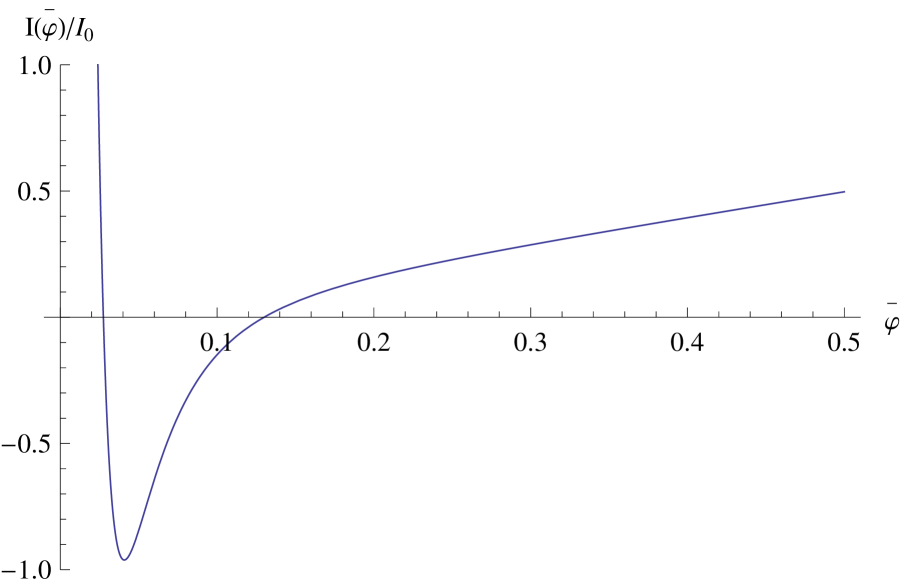
Figure 1: The average current as a function of $\bar{\varphi}$ for the condition $\nu_{0}\approx\frac{\hat{\varphi}_{1}-\hat{\varphi}_{2}}{2}\equiv\Delta=0.01$

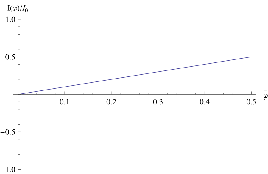
Figure 2: The average current as a function of $\bar{\varphi}$ for the case $\epsilon=0$, $\nu_{0}=\frac{\hat{\varphi}_{1}-\hat{\varphi}_{2}}{2}\equiv\Delta=0.$

References

• (1) Alexei Yu Kitaev β€β€˜Unpaired Majorana Fermions In Quantum Wires”’ cond-mat/ 0010440 and Alexei Yu Kitaev ,Ann.Phys.303,2 (2003).
• (2) D.Schmeltzer β€β€˜Topological Insulators”’-Transport In Curved Space”’ Advances in Condensed Matter and Material Research Volume 10 pp. 379-402 Editors: Hans Geelvinck and Sjaak Reynst and cond-mat/1012.5876.
• (3) D.Schmeltzer , J. Phys:Condens Matter 20 335205(2008).
• (4) D.Schmeltzer and A.Saxena ,Phys.Rev.B 81 ,195310 (2010).
• (5) S.Tewari,S.Das Sarma and Dung-Hai Lee”’ An index Theorem For The Majorana Zero Modes, In Chiral P-Wave Superconductors”’ cond-ma/0609556
• (6) Y.Oreg ,Gil Refaeli and Felix von Oppen β€β€˜Helical Liquids and Majorana Bound States In Quantum Wires”’ cond-mat/1003.1145
• (7) L.Jiang, D.Peccker,J.Alice,Gil Refaeli, Y.Oreg and Felix von Oppen cond-mat/1107.4102
• (8) D.Schmeltzer and R.Berkovits Physics Letters A 253 341-344(1999).
• (9) D.Schmeltzer β€β€˜Dirac’s Method For Constraints Quantum Wires”’ J.Phys:Condens.Matter 23 155601 (2011).
• (10) Gordon W.Semenoff and Pasquale Sodano β€β€˜ Teleportation By A Majorana Medium”’ cond-mat/0601261.
• (11) Daniel Boyanovsky Phys.Rev.B.39, 6744(1989).
• (12) D.Schmeltzer et al.,Phys.Rev.Lett90,116802(2003)
• (13) D.Schmeltzer et. al J.Phys.Condens. Matter 22, 095301 (2010)
• (14) D.Schmeltzer J.Phys.Condens. Matter 23,155601 (2011)
• (15) D.Schmeltzer and R.Berkovits Phys.Lett.A243341,(1999)