Proper motions of the Arches cluster with Keck LGS-Adaptive optics: the first kinematic mass measurement of the Arches

Abstract

We report the first detection of the intrinsic velocity dispersion of the Arches cluster - a young ($\sim$ 2 Myr), massive ($10^{4}M_{\odot}$) starburst cluster located only 26 pc in projection from the Galactic center. This was accomplished using proper motion measurements within the central $10^{\prime\prime}\times 10^{\prime\prime}$ of the cluster, obtained with the laser guide star adaptive optics system at Keck Observatory over a 3 year time baseline (2006-2009). This uniform dataset results in proper motion measurements that are improved by a factor $\sim$ 5 over previous measurements from heterogeneous instruments. By careful, simultaneous accounting of the cluster and field contaminant distributions as well as the possible sources of measurement uncertainties, we estimate the internal velocity dispersion to be $0.15\pm 0.01$ mas yr^-1, which corresponds to $5.4\pm 0.4$ km s^-1 at a distance of 8.4 kpc.

Projecting a simple model for the cluster onto the sky to compare with our proper motion dataset, in conjunction with surface density data, we estimate the total present-day mass of the cluster to be $M(r<1.0~{}{\rm pc})=1.5^{+0.74}_{-0.60}\times 10^{4}M_{\odot}$. The mass in stars observed within a cylinder of radius $R$ (for comparison to photometric estimates) is found to be $M(R<0.4~{}{\rm pc})=0.90^{+0.40}_{-0.35}\times 10^{4}M_{\odot}$ at formal $3\sigma$ confidence. This mass measurement is free from assumptions about the mass function of the cluster, and thus may be used to check mass estimates from photometry and simulation. Photometric mass estimates assuming an initially Salpeter mass function ($\Gamma_{0}=1.35$, or $\Gamma\sim 1.0$ at present, where $dN/d(\log M)\propto M^{\Gamma}$) suggest a total cluster mass $M_{cl}\sim(4-6)\times 10^{4}M_{\odot}$ and projected mass ($\sim 2\leq M(R<0.4~{}{\rm pc})\leq 3$) $\times 10^{4}M_{\odot}$. Photometric mass estimates assuming a globally top-heavy or strongly truncated present-day mass function (PDMF, with $\Gamma\sim 0.6$) yield mass estimates closer to $M(R<0.4~{}{\rm pc})\sim 1-1.2\times 10^{4}M_{\odot}$. Consequently, our results support a PDMF that is either top-heavy or truncated at low-mass, or both.

Collateral benefits of our data and analysis include: (i) cluster membership probabilities, which may be used to extract a clean cluster sample for future photometric work; (ii) a refined estimate of the bulk motion of the Arches cluster with respect to the field, which we find to be 172 $\pm$ 15 km s^-1, which is slightly slower than suggested by previous VLT-Keck measurements; and (iii) a velocity dispersion estimate for the field itself, which is likely dominated by the inner galactic bulge and the nuclear disk.

1 Introduction

The spectrum of masses produced during the star formation process (the Initial Mass Function, or IMF) is a key prediction of the star formation process as it indirectly links to the observable Present-Day Mass Function (PDMF) of the population (for example, see Miller & Scalo, 1979; McKee & Ostriker, 2007; Bastian et al., 2010, for review). Because star formation depends on collapse by self-gravity out of a turbulent medium threaded with a magnetic field, there is some expectation that the physical conditions in the parent cloud should affect the slope of the IMF, its minimum mass, or both (e.g. Morris, 1993). Numerical modeling provides some support for environment-dependent IMF variations, particularly in the unusual environment of the Galactic center (e.g. Bonnell et al., 2004; Klessen et al., 2007; Krumholz & McKee, 2008; Bonnell & Rice, 2008). However, the resulting IMF variations may be so small as to be observable only in extreme environments (e.g. Elmegreen et al., 2008). There is some observational support for a varying IMF and turn-over mass in the extreme environments of the young ($\sim$ few Myr), massive ($\sim 10^{4}M_{\odot}$) starburst clusters NGC 3603 (Harayama et al., 2008) and for the stellar cluster at the Galactic center itself (Bartko et al., 2010).

The young, massive cluster (YMC) known as the Arches Cluster (e.g. Nagata et al., 1995; Cotera et al., 1996) is a particularly well-studied example of an extreme environment for star formation. It is massive (Total mass $M_{cl}\sim(2-7)\times 10^{4}M_{\odot}$; Figer et al., 1999, 2002) dense ($\rho_{c}\sim 10^{5}M_{\odot}$ pc^-3 Espinoza et al., 2009) and young ($\sim 2-2.5$ My; Najarro et al., 2004; Martins et al., 2008). It contains a substantial number of massive stars (Serabyn et al., 1998) which both contribute to and heat the surrounding medium (e.g. Figer et al., 2002; Yusef-Zadeh et al., 2002; Lang, 2004).

The Arches cluster is located only 26 pc in projection from the Galactic center (hereafter the GC). It therefore likely formed in an environment characterised by high gas pressure and velocity dispersion in the parent cloud, and high ambient temperature, particularly when compared to the relatively more benign environment of NGC 3603. As these parameters are thought to impact the IMF (Morris, 1993; Klessen et al., 2007), the Arches cluster is expected to be an excellent candidate for observing a non-canonical IMF, whether in its mass function exponent, low-mass turnover, a low-mass cut-off, or all three (e.g. Stolte et al., 2002; Klessen et al., 2007). It is also young enough that the most massive main-sequence stars are still present, making it one of the few clusters in which the upper mass-limit to the star formation process may be observationally tested (Figer, 2005; Crowther et al., 2010). It has thus received substantial observational attention, with efforts focused particularly on estimates of its IMF. Indeed, the Arches was originally the prototypical object for a non-standard IMF (Figer et al., 1999), with an observed present-day luminosity function indicating an overabundance of massive stars compared to the canonical Salpeter IMF (parameterized as $dN/d(\log M)\propto M^{-\Gamma}$, with $\Gamma=1.35$; see Bastian et al. 2010 for a review).

However, a number of effects conspire to obscure the true IMF from observation, complicating the interpretation of the PDMF, and indeed the present consensus seems to be that the Arches began with an IMF that is consistent with the canonical Salpeter IMF found in most environments. Photometric efforts to chart the present-day luminosity function of the cluster suffer from two important limitations. Firstly, the observations are difficult; strong crowding and high, spatially-variable extinction are observed across the field of view, so that the photometric completeness is challenging to estimate for masses lower than a few $M_{\odot}$. There is evidence for mass segregation in the cluster (Figer et al., 1999; Stolte et al., 2005), seen as a steepening of the present-day luminosity function towards the cluster center, implying strong spatial selection effects when attempting to constrain the IMF.

Secondly, the relationship of the PDMF to the IMF is not trivial to evaluate. Stellar evolution must be taken into account when relating the PDMF to the IMF, requiring a prescription for mass-loss from high-mass objects (e.g., Espinoza et al., 2009). In addition, mass segregation and tidal stripping are both likely to have been important for the evolution of the Arches. Present-day mass segregation need not be primordial, since the Arches is likely already in a post-collapse phase (e.g. Portegies Zwart et al., 2007; Allison et al., 2009). The Arches cluster sits in a strong tidal field, such that as much as half of its stars may already have been stripped into the field over the $\sim 2.5$ My of its history (Kim et al., 2000; Portegies Zwart et al., 2002b). Mass segregation and tidal stripping together imply that the true IMF of the cluster may differ from the IMF drawn from the subset of stars that have remained within the Arches cluster to the present day. We review the literature mass determinations in Section 5.2.

A kinematic mass measurement provides a direct test of the PDMF of the Arches cluster, because its selection effects are somewhat less stringent. Stars below the typical photometric completeness limit of $\sim 1-2M_{\odot}$ are observable through their contribution to the total cluster mass. Figer et al. (2002) were the first to attempt this, by estimating the radial velocity dispersion of a sample of emission-line stars and assuming the cluster is spherically symmetric and in virial equilibrium. However, the estimate is complicated by the difficulty of resolving the blended lines, their high width, and intrinsic line-profile variation among the sample, so that the resulting mass estimate is strongly dependent on atmosphere models. Mass estimates using the velocity dispersion derived from proper motions are independent of the details of the atmospheres of the tracer stars, and in principle allow for the mass distribution to be derived in a more assumption-free manner (Leonard & Merritt, 1989).

The advent of adaptive optics on large telescopes in the near-infrared has enabled the measurement of precise proper motions of a large number of stars in the Galactic center clusters. In a pioneering proper motion study of the Arches, Stolte et al. (2008) used one epoch each of VLT/NACO and Keck/NIRC2 separated by 4.3 years to measure the motion of the cluster. However, differential distortion between the cameras limited the proper motion precision to $\sim 0.7$ mas yr^-1, somewhat too coarse to measure the internal velocity dispersion, for which the expected order of magnitude is about $\sim 0.2$ mas yr^-1.

We have observed the central $10^{\prime\prime}\times 10^{\prime\prime}$ of the Arches across five epochs in three years (2006-2009) with a uniform observational setup (PI Morris). Using NIRC2 on Keck-2, behind the LGS Adaptive Optics facility (Ghez et al., 2005; Wizinowich et al., 2006), these cross-instrument systematics encountered by Stolte et al. (2008) are not present in our observations, and we are able to attain proper motion measurements with error lower than the expected velocity dispersion. We report here on our results, which provide the first kinematic mass estimate of the Arches cluster from proper motions.

This communication is organised as follows. Section 2 describes the observations and positional measurement technique, while Section 3 describes the process of proper motion measurement and error assignment. Section 4 describes the techniques used to fit the cluster membership probabilities and kinematic parameters. Section 5 provides our mass measurement and new bulk motion measurement for the Arches, and briefly discusses the implications.

2 Observations & Measurements

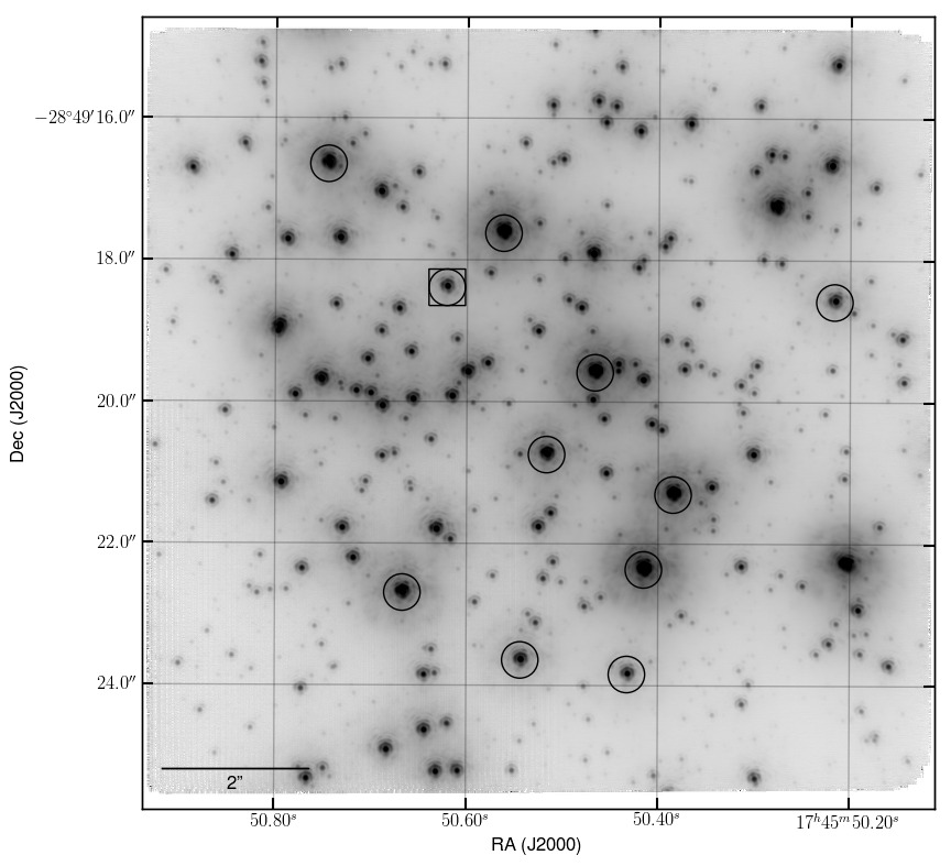
Observations of the central $10^{\prime\prime}\times 10^{\prime\prime}$ of the Arches cluster were obtained between May 2006 and May 2009 with the Keck near-infrared camera (NIRC2: PI K. Matthews), behind the Laser Guide Star Adaptive Optics (LGSAO; van Dam et al., 2006; Wizinowich et al., 2006) system on the W. M. Keck II 10-meter telescope. All observations were obtained with the narrow-field mode of NIRC2 (field of view $10.2^{\prime\prime}\times 10.2^{\prime\prime}$), which has a pixel scale of 9.952 $\pm 0.003$ mas pix^-1 (Yelda et al., 2010, hereafter Y10). Observations were taken in the $K^{\prime}$ filter ($\Delta\lambda=0.35\mu m$, $\lambda_{0}=2.12\mu m$). Five epochs of the central field in $K^{\prime}$ have now been taken (Table 1), the second of which (2006 July 18) was first reported in Stolte et al. (2008). Observations were designed to be as uniform as possible across the epochs, with detector-Y commanded to align with the S-N direction at each epoch, with the same pseudorandom dither pattern within a $0.7^{\prime\prime}\times 0.7^{\prime\prime}$ box applied at each epoch (Ghez et al., 2008), and with observations taken at pointings with as uniform a range of zenith angles as practical. Three images were taken at each position within the dither pattern. Figure 1 shows the mean image constructed from the May 2009 dataset. This is our best map in terms of both angular resolution (FWHM 51 mas) and sensitivity ($K^{\prime}_{lim}=20.59$ mag; Table 1). Table 2 shows the PSF stars used in the analysis.

3 Analysis

Our goal is to extract relative proper motions of Arches stars against the field, which is mostly composed of bulge stars. The analysis proceeds in the following stages: (1). Positions are estimated from a master-image at each epoch (Section 3.1). (2) The extracted positions are transformed into a reference frame common to all epochs using likely cluster members, and proper motions extracted from the positional time-series in this frame, using statistical uncertainties (Section 3.2). (3) Possible sources of additional proper motion uncertainties are explored (Section 3.3) and, when such additional error sources are identified, motions are re-extracted incorporating the updated errors. Section 3.3 briefly discusses the proper motion precision attained.

3.1 Production of star-lists from each epoch

The procedures used by our group to produce lists of stellar positions and fluxes from the image-sets at each epoch have been fully described elsewhere (Ghez et al., 2008; Lu et al., 2009; Yelda et al., 2010); here we recapitulate briefly the aspects relevant for the present work. Images are calibrated and corrected for differential atmospheric refraction, and corrected for static distortion using the most accurate distortion characterization currently available (Y10). Within an epoch, the corrected images are combined into a mean image using positional shifts only, weighting by the Strehl ratio estimate for each image. Images are combined using the Drizzle algorithm (Fruchter & Hook, 2002), and the mean frame is not supersampled since the pixels already provide 2.5$\times$ Nyquist sampling. This is in contrast to common practice when using Drizzle with Hubble data, which is typically only barely Nyquist sampled. The shifts to use are estimated using cross-correlation of the scene between images. By combining using shifts only, we average through any rapid variations in instantaneous distortion, and average over slow drifts in image orientation, which, based on transformations between ccommon stars across a set of images within the night, appear to be only $\sim 1^{\prime}$ over the course of a night and are therefore negligible. A modified version of the IDL routine Starfinder (Diolaiti et al., 2000) is then used to measure star positions in the mean frame (Y10 & refs. therein) by simultaneous fitting of the point-spread function (herein PSF) to many stars. In each epoch, 500-900 stars are identified, depending on the performance of the AO system and the number of frames collected (Table 1).

Within an epoch, the positional estimate for each star is associated with random measurement uncertainty on the mean of all images within the night that passed quality control (we call this random uncertainty the “centroiding uncertainty;” see Section 3.3.1 for details on its measurement).

3.2 Transformations to common reference frame and proper motion measurement

The Arches cluster moves rapidly with respect to the field ($\sim 5$ mas yr^-1), shows low velocity dispersion compared to that of the field, and accounts for most of the stars in the field of view (Stolte et al. 2008). We therefore measure motions in the reference frame in which the cluster is at rest. Details of this process are given in Appendix A; here we outline the important considerations.

First, stars are matched across epochs to produce a master catalogue containing all the original position measurements of each star. Each star-list is transformed to the frame of a single star-list at a chosen epoch $t_{0}$. Motions are estimated from straight-line fits to the transformed measurements in $t_{0}$. These measurements are then used to construct a refined cluster reference frame at a chosen time $t_{ref}$ and the original star-lists are then re-mapped onto this refined frame and proper motions re-evaluated in this frame.

The choice of epoch $t_{0}$ is determined by the data quality and by the epochs of observation. Proper motions are determined from straight-line fits to positions in the chosen reference frame; choosing a reference frame near the pivot point of these straight line fits will minimize the error when mapping star-lists. Of the three deepest epochs (Table 1), epoch 2008.5 is closest to this pivot point, and is adopted as $t_{0}$. Once a first estimate of proper motions has been produced in this reference frame, the distribution of pivot points of the first pass at straight-line fits is assessed; its mode is $t_{ref}$ =2008.0. The reference frame for motions is then constructed by evaluating the fits to the positional time-series from the first pass, at time $t_{ref}$ .

Because the field and cluster populations show significantly different motion, field stars are removed from consideration when evaluating the transformation parameters that map reference frames onto each other. This is achieved by clipping outliers in the vector point diagram; after a few iterations of clipping and re-fitting, the centroid of the cluster population is at zero motion in the vector point diagram.

When mapping star-lists between epochs, the transformation parameters are estimated by $\chi^{2}$ minimization using the positional differences in each coordinate separately. The appropriate order of transformation - a second-order polynomial - was determined by evaluating the positional residuals as a function of order (Appendix C). Transformation parameters are given in Table 3.

Measurements are inverse-variance weighted using the error estimates in each coordinate for each star. As part of the fitting, three passes of sigma-clipping (with 4$\sigma$ bounds) are used to reduce sensitivity to measurement-outliers, mismatches or misidentification of cluster members among the reference stars. This typically removes a few stars from the reference list used for the mapping and can be regarded as a fine-tuning of the reference star list for a given mapping.

As the analysis proceeds, additional estimates of positional error become available to use as weights (see Section 3.3). When mapping star-lists onto each other, errors used in the weighting are the positional errors associated with each star-list. When mapping star-lists onto the reference frame $t_{0}$, these errors are just the centroiding error in each list; when mapping onto $t_{ref}$ the errors associated with the target frame are the errors in the predicted position in $t_{ref}$ based on the first pass of motion estimation. When evaluating velocities in a given frame, the positional error and error associated with the mapping into this frame (the alignment error; Section 3.3.2) are added in quadrature. Measured velocities are then used to investigate any additional error not taken into account. Upon discovery of an error source missing from the analysis, the entire analysis is repeated with the missing error term included. Additional random error determined from the velocity fits is associated with random variations in position-measurement of a given source between epochs, and so is added in quadrature to the centroiding error in the frame mapping and subsequent mapping. The size of this additional error is examined in Section 3.3.3.

3.3 Positional and Motion errors

We now describe the error sources that are included in our analysis in some detail.

3.3.1 Centroiding error

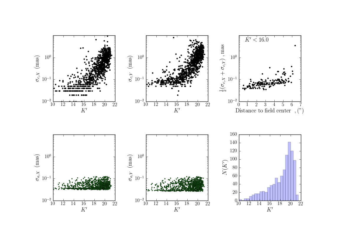
The centroiding uncertainty (random error in position-measurement on the mean image from an epoch) is estimated empirically. The stack of images from each epoch is divided into three subsets of equal length, yielding three “submaps” - mean images of each of the three subsets. Images are sorted in decreasing order of Strehl ratio and each submap constructed from every third image surviving quality control in the resulting list. Each submap has therefore been formed from images spanning the same range of observationally relevant conditions (such as Strehl ratio and pointing). Because each submap describes a similar path through auxiliary parameter-space both in relation to each other and to the mean image from the night, images are mapped onto the same reference frame using simple translations before averaging into a submap in the same manner as the production of the mean image. Positions are also measured on each of the three submaps in the same way as for the mean image, and these positions then mapped onto the reference frame of the mean image using shifts only. This produces three position measurements from the night, each using one third of the information from the night and taking the same path through auxiliary parameter-space. The rms of stellar position measurements across the three submaps is evaluated for each star to estimate the random error on the mean of one third of the images within the night. This must be scaled by $1/\sqrt{3}$ to estimate the centroiding error from the mean image for the star in question. For stars brighter than $K^{\prime}=16$, this centroiding uncertainty is typically 0.1 mas (Table 4 and Figure 2).

3.3.2 Alignment error

Error in predicted positions due to the mapping between frames was estimated through Monte Carlo resampling: sets of half the reference stars were randomly drawn and the frame-mapping re-fit and re-evaluated for each trial set to produce a trial set of positions as transformed into the target frame. The rms of the differences between these predicted positions and those predicted from the full list is then adopted as the contribution to random positional error due to the fitting process. This error is always included when positional errors after transformation are needed (steps 4 and onward in Appendix A). Figure 2 shows the typical magnitude of alignment errors.

3.3.3 Additional random errors

When velocities were extracted, the distribution of $\chi^{2}$ values from the velocity fits is quite different from that expected if all random errors had correctly been included (Appendix B); clearly additional positional variation is present between epochs that is not accounted for by centroiding and alignment error alone. To properly represent random error along each positional time-series, an additional temporally-random error $\delta$ (denoted here as “additive error”) must be added in quadrature to the random error sources estimated thus far. The size of additive errors $\delta_{x},\delta_{y}$ required (after accounting for higher-than-linear frame-to-frame transformations; see below) are determined by Maximum Likelihood, as detailed in Appendix B1. We find that a flat distribution of additive error with magnitude produces a velocity $\chi^{2}$ distribution significantly more discrepant from statistical expectation than a magnitude-dependent additive error (Appendix B2). We therefore adopt estimates of $\delta_{x},\delta_{y}$ that vary with magnitude (see Table 4; specifically, for $K^{\prime}<16$ the values are $\delta_{x},\delta_{y}=0.16,0.15$ mas).

While the balance of important terms varies across different facilities, the major causes of additional error are discussed in some detail by Fritz et al. (2010); we give three example causes here that cannot practically be overcome by experimental design. (i) The AO-corrected PSF core sits on top of a broad halo with radius similar to the seeing radius ($\sim$1/20^th the size of the entire field of view), resulting in significant background spatial structure. Because the spatial scale of this structure is a significant fraction of the field of view, and the field itself is highly crowded, astrometric error due to seeing halo bias is difficult to model with high accuracy. As the seeing halo depends on seeing conditions during the observation, it varies between epochs and therefore manifests itself as an additional time-random error component . (ii) Related to this is source confusion, where the PSF of an object of interest overlaps that of another object (resolved or unresolved); the magnitude and direction of the bias depends on the relative brightness of the two objects and on the spatial structure of the PSF. Note that this astrometric bias may vary systematically with time (due to time-varying object separation due to object relative motion; e.g. Ghez et al. 2008), or randomly with time due to variation in the PSF structure between epochs (which we assume to be temporally random on timescales of months-years). This confusion-error may be spatially correlated if the variation of the PSF between epochs is spatially-correlated. (iii) The distortion suffered along the path from source to pixels may vary between epochs in a number of ways, producing spatially correlated but temporally-random spurious apparent motions between epochs. For example: the mean reference frame within an epoch is constructed from a strehl-weighted sum of instantaneous images, and therefore depends on the time-variation of observing conditions throught the night, which varies between epochs. Thus, a variation in distortion may be expected between epochs even in the limit of a perfectly stable instrument and telescope. Of the three error-sources above, source confusion (source ii) is expected to vary the most strongly with target object magnitude, and thus is a strong candidate for the additive error $\delta_{x}$, $\delta_{y}$.

3.4 Resulting Proper motion precision

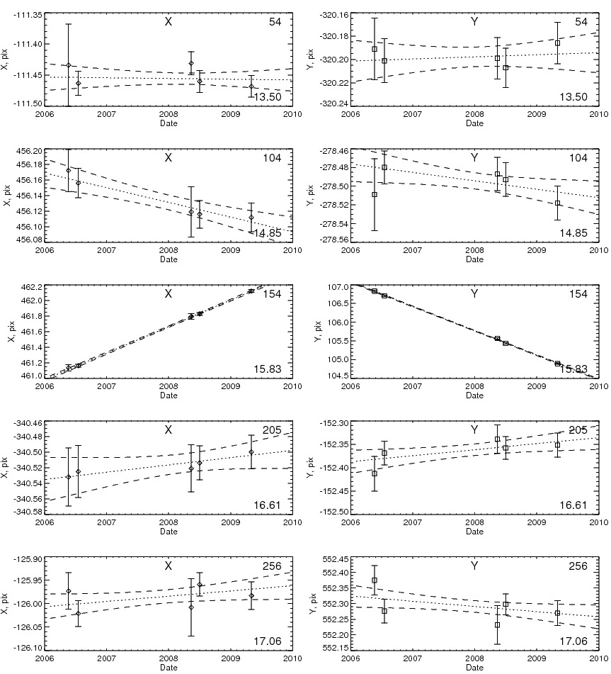
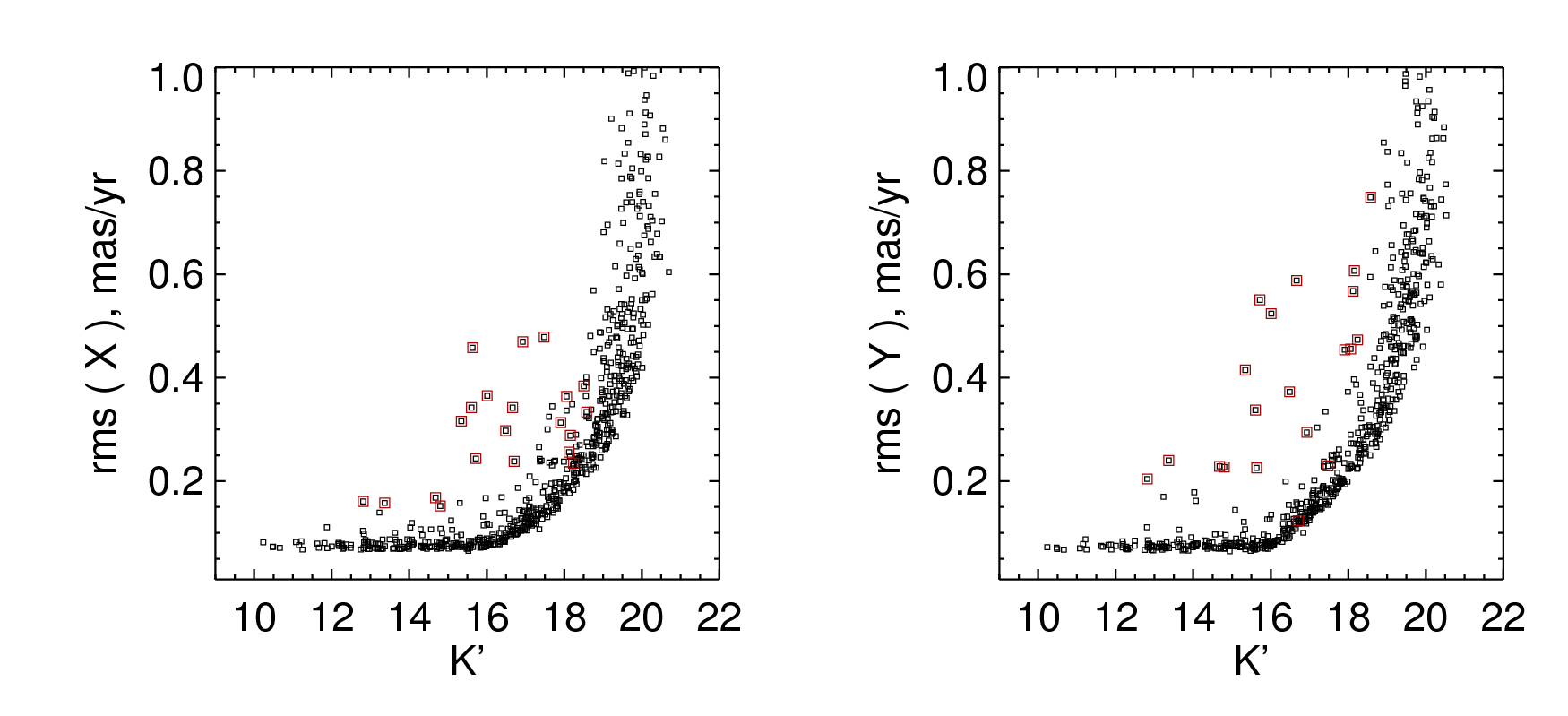
We have achieved proper motion precision sufficiently high to measure intrinsic dispersion. Positional time-series for a selection of objects, along with the motions fitted to the time-series of the objects, are provided in Figure 3. The proper motion precision adopted is shown in Figure 4. Table 4 summarises the error budget of our astrometric measurements.

4 Results

The cluster shares the field of view with a significant field population. To estimate membership probabilities, we fit the kinematic parameters of the cluster and field components simultaneously with the relative contribution each component makes to the population in the image (Section 4.1.1). Armed with membership probabilities, we also estimate the velocity dispersion of the cluster and subsamples within the cluster by direct Maximum Likelihood fitting of the motions of likely cluster members (Section 4.1.2). Section 4.2 discusses the velocity dispersions resulting from each approach. Since the two approaches produce similar estimates for the dispersion, we re-express velocities in terms of radial and tangential components in order to calculate the proper motion dispersion profile for use in mass modeling (Section 4.3).

4.1 Membership Probabilities from kinematic fitting

Table 5 provides a complete catalogue of formal membership probabilities for cluster and field for all 432 objects surviving the culls in Appendix A and for which five epochs of position-measurement are available. Given best-fit kinematic parameters, the probability that a given star is a member of the $k$’th kinematic component, is then the usual

$$P(k)_{i}=\frac{\phi_{ki}}{\sum^{K}_{j}\phi_{ji}}$$ (1)

where $\phi_{ki}$ gives the likelihood that the $i$‘th star belongs to the $k$‘th component, and depends on the fit to the kinematic parameters of the field and cluster. We describe the process of obtaining $\phi_{ki}$ below.

4.1.1 Kinematic fitting

Too few field objects are present in our sample to decompose the field population by distance based on our measurements, so we appeal to the literature. The field population is likely dominated by stars in the inner region of the Milky Way bulge and may contain some population from the outer regions of the nuclear stellar disk (hereafter NSD; Launhardt et al., 2002). Both the bulge and NSD should show some degree of central concentration along our line of sight (however, not necessarily centered on the distance of the Arches; see Section 5.3). For the bulge we expect to preferentially sample field stars within a few hundred parsecs of the Arches population itself along the line of sight (e.g., Cabrera-Lavers et al., 2007). The velocity signature of the field component should thus be a sum of differential rotation along the line of sight and intrinsic velocity dispersion, sampled from the bulge and NSD. The contributions of the NSD and galactic bulge to the field of the arches may be comparable in size (e.g. Figure 2 of Launhardt et al. 2002), however the uncertainty in the mass model in the inner regions is still rather large. For the purposes of this work, we parameterize the sum of bulge + NSD as a single two-dimensional Gaussian within the VPD.

Unlike many cluster studies (e.g., Platais et al., 2003), our field component is expected to be significantly asymmetric in the vector point diagram (hereafter VPD), as the bulge velocity dispersion is larger along the galactic plane than perpendicular to it (Kuijken & Rich, 2002); at 350pc from the Galactic center, for example, proper motion dispersions are of order $5$ and $3$ mas yr^-1 along and perpendicular to the galactic plane, respectively (Clarkson et al., 2008).

Because the cluster distribution in the vector point diagram is so much tighter than the field distribution, fitting to the binned VPD is not appropriate for this dataset as there is no binning factor that allows simultaneous resolution of both cluster and field components. Instead we maximize the likelihood $L$(data given the component fractions, kinematic parameters, measurement errors) without recourse to binning. The component fraction $\pi_{k}$ describes the proportion of the sample of tracer stars in the image that belong to the $k$’th kinematic component. Since our field fits entirely within the flat core of the surface density radial profile (Espinoza et al. 2009), we assume that $\pi_{k}$ is uniform within our field of view.

We follow standard practice (e.g., Sanders, 1971; Jones & Walker, 1988; Kozhurina-Platais et al., 1995) in using a two-dimensional gaussian profile to model the intrinsic kinematic properties of the cluster in the VPD. The field population is likely to be dominated by bulge objects which occupy a rather narrow distance range compared to the distance to the Galactic center; we therefore parameterize the field component with a two-dimensional gaussian. Because the convolution of two bivariate gaussians is another bivariate gaussian, whose covariance matrix is the sum of those of the two components, this choice of model form allows errors to be included naturally in the analysis. The likelihood of finding a star at a given location in the VPD is thus given by the sum of $K$ gaussian components:

$$L(\vec{v_{i}}) = \sum^{K}_{k}\pi_{k}\frac{1}{2\pi|{\bf\Sigma}_{ki}|^{1/2}}\exp{\left(-\frac{1}{2}(\vec{v_{i}}-\bar{\mu_{k}})^{T}{\bf\Sigma}_{ki}^{-1}(\vec{v_{i}}-\bar{\mu_{k}})\right)}$$ (2)

$$\equiv \sum^{K}_{k}\phi_{ki}$$

where $\phi_{ki}$ describes the likelihood of finding a given star in a given component at its measured location in the VPD. In (2), $\overline{\mu_{k}}$ is the centroid of the $k$’th component in the VPD and ${\bf\Sigma}_{ki}$ the covariance of the $k^{\prime}th$ component for the $i$’th star. Because the kinematic model and error model are both gaussian, the covariances due to error and model combine in the form ${\bf\Sigma}_{ki}={\bf S}_{i}+{\bf Z}_{k}$, where the diagonal positional-error matrix ${\bf S}_{i}$ has components ($\sigma^{2}_{v,x},\sigma^{2}_{v,y}$) and the covariance matrix of the $k$’th model component is given by ${\bf Z}_{k}$.

Once the best-fit ${\bf\Sigma}_{ki}$ has been estimated from the proper motion data and errors, the intrinsic velocity dispersions $\sigma_{a},\sigma_{b}$ and the major-axis orientation $\theta$ of each component are found from the eigenvalues and eigenvectors of ${\bf\Sigma}_{ki}-{\bf S}_{i}$.

Best-fit parameters and component fractions are found by maximizing $\sum^{N}_{i}\ln L(\vec{v_{i}})=\sum^{N}_{i}\ln\left(\sum^{K}_{k}\phi_{ik}\right)$ over the sample of tracer stars of interest, under the constraint $\sum^{K}_{k}\vec{\pi}_{k}=1$. The maximum-likelhood $\pi_{k}$ and the kinematic parameters are evaluated sequentially and iteratively until convergence. If the errors are constant over the sample of interest (so ${\bf\Sigma}_{ki}\approx{\bf Z}_{k}+\bar{\bf S}$), then each update step requires the evaluation of analytic expressions for the maximum-likelihood estimate of the updated $\pi_{k}^{\prime}$ given the current estimate of the parameters (and vice versa). This is the well-known Expectation Maximization (hereafter EM) algorithm. This technique is well-established outside astronomy (Chapter 9 of Bishop 2008 provides a thorough explanation, and the method has appeared in the most recent edition of Press 2002) and is becoming more commonly employed to mixture problems in astronomy in which binning is undesirable and/or a low number of reference objects is available (Bovy et al., 2009).

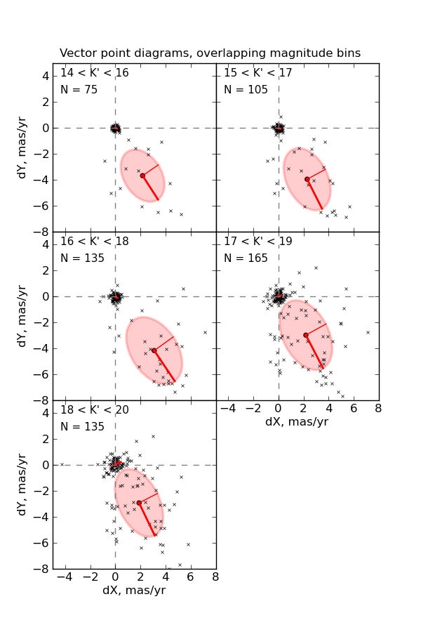
Strongly-varying error on a star-by-star basis is a significant complication, as the parameter-update step no longer has an analytic form, and instead must be solved numerically. For the present investigation, we use a single cluster component and choose instead a variant of the technique of Kozhurina-Platais et al. (1995, and refs. therein) in which membership probabilities for each star are estimated using kinematic parameters fitted only from stars with roughly similar error (so ${\bf\Sigma}_{ki}\approx{\bf Z}_{k}+\bar{\bf S}={\bf\Sigma}_{k}$ for the sub-sample). The sample is broken into overlapping bins two magnitudes wide (so $K^{\prime}$=14.0-16.0, 15.0-17.0, 16.0-18.0 and 17.0-19.0) and the best-fit parameters determined for each magnitude strip separately (Table 6 and Figure 5). Investigation of remaining magnitude-dependent bias can be found in Appendix D. We find that parameters do not become strongly affected by bias until stars as faint as $K`=18$ are considered.

Between $15\leq K^{\prime}<18$, every star is at most half a magnitude from the center of one of the magnitude-strips, and it is the parameters corresponding to this nearest magnitude-strip that are used to evaluate (1) for these stars. Objects at $K^{\prime}<15.0$ use the kinematic parameters evaluated for $K^{\prime}<16.0$ (see also Section 4.1.2), while objects at $K^{\prime}>18.0$ use the kinematic parameters estimated from $17.0\leq K^{\prime}<19.0$.

Errors on the parameters thus fit are estimated by Monte Carlo bootstrap analysis. The observed vector point diagram is resampled by random drawing of points from the full sample with replacement. The full kinematic fitting process is re-applied to each trial and the distribution of recovered values parameterized with its standard deviation about the mean value using the full dataset.

4.1.2 Direct calculation of the velocity dispersion

The process given in Section 4.1.1 fails when the sample size is small (i.e. $\lesssim$ 70 stars), or contains a negligible field component (as occurs for $K\lesssim 14.5$). Our end goal is to compute the dispersion profile as a function of distance from the cluster center for mass modeling, which may entail few stars per annulus. We therefore compute the velocity dispersion from proper motions using a direct Maximum Likelihood approach. Likely-cluster objects are isolated using the membership probabilities estimated from the fits of the previous section. Along each direction, we maximize

$$L(\overline{v},\sigma)=\prod^{N}_{i}(2\pi(\sigma^{2}+e^{2}_{i}))^{-1/2}\exp\left\{-(v_{i}-\overline{v})^{2}/2(\sigma^{2}+e_{i}^{2})\right\}$$ (3)

for $\overline{v},\sigma$ iteratively, where $\sigma$ is the intrinsic velocity dispersion and $e_{i}$ the measurement error. For each $\sigma$, $\overline{v}$ is obtained by weighted averaging while for each $\overline{v}$, $\sigma$ is found numerically by bisection. Errors are estimated by Monte Carlo bootstrap analysis; members of the sub-sample are drawn randomly with replacement and the calculation repeated for a large number of trials. The standard deviation of the fitted parameters across the set of trials is then adopted as the fitting error from this process. Table 7 shows the dispersions and their errors estimated by this procedure.

4.2 Cluster Velocity Dispersion

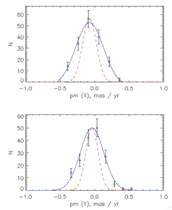
The kinematic fitting (Section 4.1.1) and direct (Section 4.1.2) approaches produce complementary estimates for the intrinsic velocity dispersion of the Arches cluster. Both have been corrected for measurement error using the procedures described above. Tables 6 & 7 show the kinematic parameters fit to cluster and field, and the velocity dispersion estimate for the cluster respectively. Figure 6 shows the velocity dispersion graphically and its comparison to the proper motion error.

Both estimates yield statistially significant measurements of the cluster velocity dispersion. The mean cluster velocity dispersion and its error is estimated by inverse variance-weighted average of the determinations from non-overlapping magnitude bins, for $K^{\prime}<18.0$ (to avoid strong error and mass segregation effects). For the dispersions estimated from the kinematic fitting (Section 4.1.1; Table 6), magnitude bins $(14.0\leq K^{\prime}<16.0)$ and $(16.0\leq K^{\prime}<18.0)$ are used. We do not use the magnitude bin $K^{\prime}>18.0$ because this bin appears to suffer misclassification bias under the fitting technique used; see Appendix D.

This yields mean velocity dispersions along major and minor axes respectively, of ($\overline{\sigma_{a}},\overline{\sigma_{b}})=(0.154\pm 0.01,0.136\pm 0.008)$ mas yr^-1. Scaling to the distance of the Galactic center ($8.4\pm 0.4$ kpc; Ghez et al. 2008) this yields measured velocity dispersion $(5.8\pm 0.48,5.2\pm 0.40)$ km s^-1.

For the dispersions estimated directly from likely cluster members in each direction separately, (Section 4.1.2 and Table 7), the mean velocity dispersions in the three non-overlapping bins brighter than $K^{\prime}=18.0$ are $(\overline{\sigma_{x}},\overline{\sigma_{y}})=(0.149\pm 0.011,0.124\pm 0.016)$ mas yr^-1, which translates to velocity dispersion ($5.7\pm 0.51,4.68\pm 0.65$) km s^-1 along detector XY coordinates.

Included in Table 6 is the position-angle (East of North in the VPD) of the major axis of the cluster component (denoted $\theta_{cl}$). Comparing independent magnitude-bins, we see that the orientation of the cluster major axis changes from $70.2\arcdeg\pm 21.7\arcdeg$ to $67.5\arcdeg\pm 48.3\arcdeg$ to $114.0\pm 66.4\arcdeg$ as fainter magnitude-bins are considered. Such an extreme variation indicates the apparent variation in the cluster major axis orientation is likely a sampling artifact, and does not reflect underlying variation. The detector X and Y directions therefore sample a symmetric distribution in two directions that are arbitrary with respect to the cluster velocity distribution. We can therefore compare the two measures by averaging the major and minor axes from kinematic fitting to make a direction-invariant measure from kinematic fitting, and average the directly-calculated dispersions along the two detector directions to form a second direction-invariant dispersion measure. This yields mean velocity dispersions $5.4\pm 0.3$ km s^-1 and $5.5\pm 0.4$ km s^-1 respectively for dispersions estimated from kinematic fitting $(14.0\leq K^{\prime}<18.0)$ and those estimated directly from cluster members ($10.0\leq K^{\prime}<18.0$).

4.3 Velocities for mass estimates

Sections 4.1.1 & 4.1.2 establish that mixture-modeling (used to establish membership probabilities) and direct calculation from cluster members produce the same estimate of the dispersion. To be compatible with mass estimates based on kinematic modeling, proper motions expressed in components aligned with the detector axes, are converted into proper motion components along the radial vector away from the cluster center, and along the vector tangential to it. Specifically, the velocities and their errors used for mass estimates, $v_{R},v_{T},\delta_{R},\delta_{T}$, are computed from the following relations:

$$\theta \equiv \arctan{\frac{Y_{\ast}-Y_{0}}{X_{\ast}-X_{0}}}$$

$$v_{R} = v_{X}\cos\theta+v_{Y}\sin\theta$$

$$v_{T} = -v_{X}\sin\theta+v_{Y}\cos\theta$$

$$\delta^{2}_{R} = \delta_{X}^{2}\sin^{2}\theta+\delta_{Y}^{2}\cos^{2}\theta$$

$$\delta^{2}_{T} = \delta_{X}^{2}\cos^{2}\theta+\delta_{Y}^{2}\sin^{2}\theta$$ (4)

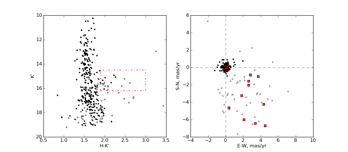
where $v_{X},v_{Y},\delta_{X},\delta_{Y}$ are the velocities and their errors along detector-X and detector-Y that were estimated from proper motions. The positions $X_{\ast},Y_{\ast}$ denote the position of the star on the detector, and $X_{0},Y_{0}$ the location of the cluster center on the detector. The sample is then broken into concentric annuli, and the velocity dispersion and its error within each annulus computed by the method of Section 4.1.2. To select a sample of cluster member stars, formal membership probabilities $P_{cluster}>0.995$ were used (see Figure 7 for an illustration of the VPD and CMD using this membership probability as a cutoff).

The cluster center itself is not apparent as a peak in individual motions or surface density within the restricted field of view of our central-field observations (compare with Espinoza et al., 2009; Anderson & van der Marel, 2010), although the dynamical center of the cluster probably is within the rough center of our field of view. Four randomly-chosen locations for the cluster center $X_{0},Y_{0}$ are chosen (Table 8), all within 2.6” from the center of the field. Mass limits reported in Section 5.1 are taken from the ensemble range over all four choices of cluster center; in practice, the range of derived masses is not strongly dependent on the location of the cluster center.

5 Discussion

A key goal of this work is to compare mass limits set by proper motion dispersion measurements to literature mass estimates. The set of literature mass estimates is quite heterogeneous, so some discussion of notation is in order before proceeding. We use $\Gamma_{0}$ to represent the IMF slope where quoted in the cited report, and $\Gamma$ to represent the present-day mass function; both exponents refer to the form $dN/d(\log M)\propto M^{-\Gamma}$. Simulations (e.g., Kim et al., 2000; Kim & Morris, 2003) suggest that the Arches may have lost about half its mass since formation due to dynamical effects; we therefore distinguish between present-day mass $M_{cl}$ and initial-mass $M_{0}$ in the following discussion. We use radius $r$ to refer to a distance from the cluster center in three dimensions and $R$ to refer to distance from the cluster center as projected onto the sky. The term “half-mass radius” refers to the radius within which half the cluster mass is found, but the precise meaning of this term often depends on the application. In our notation, $r_{hm}$ refers to the radius of a sphere within which half the cluster mass is contained (the sense often used by theorists; Portegies Zwart et al., 2010) and $R_{hm}$ is the radius of a cylinder oriented along the line of sight, within which half the cluster mass (usually the mass of the directly-observed tracer stars) is observed. This latter quantity is the half-mass radius most commonly seen in observational estimates. Where a total cluster mass is reported, we denote it as $M_{cl}$ or $M_{0}$; where mass within a given projected radius is reported as $M(R<0.4~{}{\rm pc})$  so that the outer radius limit is clear. Throughout this report the term “projected mass” refers to the mass within a cylinder of radius $R$ on the sky whose long axis is aligned along the line of sight.

5.1 Velocity dispersion and mass

The only previous use of stellar motions to estimate the mass of the Arches of which we are aware, is that of Figer et al. (2002). Radial velocities of eight emission-line stars within $R=0.23$ pc of the cluster center were used to place an upper limit on the one-dimensional velocity dispersion. Their 22 km s^-1 was converted to an upper limit on the enclosed mass using the Virial theorem; a spherically symmetric, gravitationally-bound cluster with this velocity dispersion would have enclosed mass $M_{cl}(r<0.23~{}{\rm pc})=7\times 10^{4}M_{\odot}$. For such massive stars with strong stellar winds, interpretation of the line profile shape to estimate systematic velocities is strongly dependent on model atmospheres for massive stars (Figer et al., 2002).

A mass estimate based on proper motions is independent of the details of the line profile of the young, massive stars to which we are sensitive. We choose not to employ the moment-based kinematic mass estimator of (Leonard & Merritt, 1989, hereafter LM89), since its power to estimate the total mass given the projected-radial coverage is strongly sensitive to the outer radius-limit (e.g. Figure 11 of Schödel et al. 2009).

The method used is as follows: we start with a model for the mass density profile $\rho(r)$ of the cluster, whose parameters are varied to evaluate the comparison to our proper motion-based dispersion estimates. Several model choices are possible. We choose to use the King (1962) prescription to describe the radial density profile $\rho(r)$ of the cluster. Our choice is motivated by three observations from the literature. Firstly, the Arches cluster is likely already in a post-collapse phase; simulations suggest that for the Arches cluster, core collapse takes place only about 0.6 Myr after formation (Kim et al., 1999). This collapse erases the signature of substructure in the parent cloud and leads to cluster relaxation on a shorter timescale than the initial half-mass relaxation time. Secondly, the resulting cluster undergoes dynamical mass segregation on a timescale of 1-2 Myr, much shorter than suggested by the current crossing-time of most stars in the cluster (Allison et al., 2009). The cluster is thus much older dynamically than its current crossing time would suggest (Bastian et al., 2008; Allison et al., 2009). This suggests that a model assuming a relaxed cluster should be a reasonable first approximation to the Arches, even given its young age. Thirdly, the observed surface density profile $\Sigma(R)$ (units stars pc^-2) of massive stars ($M>10M_{\odot}$) is indeed reasonably well-fit by a King (1962) profile (Espinoza et al., 2009).

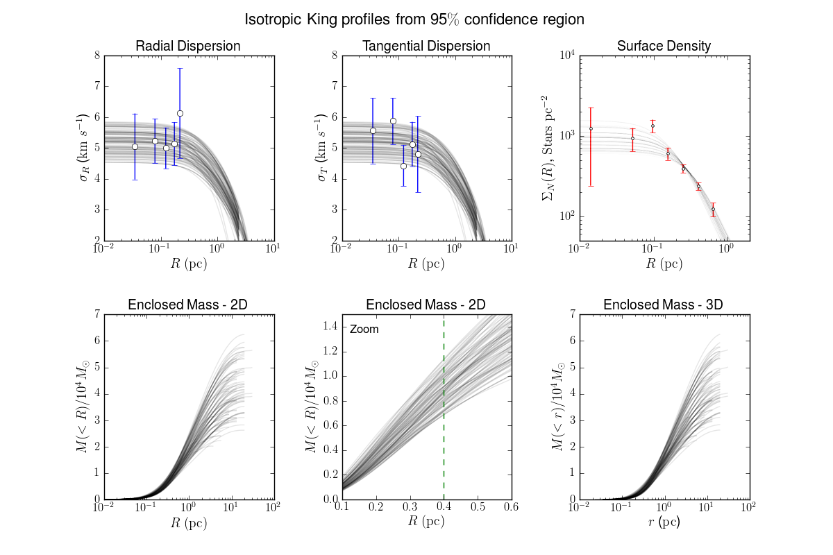
To use the King (1962) model to predict observed velocity dispersions, we make four further assumptions; we anticipate that the next step in the analysis will be to move straight to full numerical modeling of the cluster, but that is beyond the scope of this communication. We assume that the cluster is (i) not rotating strongly; (ii) can be characterized as being in equilibrium, (iii) has spherical symmetry, and (iv) shows isotropic motion. Assumption (ii) allows us to use the Jeans equation to predict the velocity dispersion profile $\sigma^{2}(r)$ corresponding to each model parameter-set. This profile is then projected onto the sky to predict the observed velocity dispersion components parallel and perpendicular to the radial direction away from the cluster center. This prediction is compared to observations (Section 4.3), and a figure of merit ($\chi^{2}$) evaluated for each set of parameters. The set of $\chi^{2}$ values mapped out in this way is used to derive confidence limits for the model parameters. Finally, confidence limits on the model parameters are converted into confidence limits on parameters of interest derived from the model - particularly the projected mass estimate $M(R<0.4~{}{\rm pc})$ .

We begin with the predictions for intrinsic velocity dispersion by substituting the model for $\rho(r)$ into the isotropic Jeans equation. Specifically, we have for the mass density $\rho(r)$ and the surface density (by mass) $\Sigma(R)$:

$$z^{2} \equiv \frac{r_{c}^{2}+r^{2}}{r_{c}^{2}+r_{t}^{2}}$$

$$\rho(r) = \frac{K}{\pi r_{c}\left[1+(r_{t}/r_{c})^{2}\right]^{3/2}}\frac{1}{z^{2}}\left(\frac{1}{z}\arccos z-\sqrt{1-z^{2}}\right)$$

$$\Sigma(R) = K\left(\frac{1}{\left[1+(R/R_{c})^{2}\right]^{1/2}}-\frac{1}{\left[1+(R_{t}/R_{c})^{2}\right]^{1/2}}\right)^{2}$$ (5)

where $r_{c},R_{c}$ refer to the core radius, $r_{t},R_{t}$ refer to the tidal radius, and lowercase/uppercase radii denote the radius in three dimensions or projected on the sky, respectively. The Jeans equation takes the form

$$\sigma^{2}_{iso}(r) = \frac{1}{\rho(r)}\int^{+\infty}_{r}G\frac{\rho(r)M(<r)}{r^{2}}dr$$ (6)

$$= \frac{G}{\rho(r)}\int^{+\infty}_{r}\frac{\rho(r)}{r^{2}}\int^{r}_{0}4\pi r^{\prime 2}\rho(r^{\prime})dr^{\prime}dr$$

which is readily evaluated numerically. This model dispersion profile is projected onto the sky using equations (8) and (10) of LM89 for comparison with observational data.

With this choice of model, three parameters determine the density profile, the dispersion profile and therefore the derived masses of interest: the core radius $r_{c}$, the tidal radius $r_{t}$ and the total cluster mass $M_{cl}$. The latter parameter is used to normalize the model through the condition

$$M_{cl}=4\pi\int^{r_{t}}_{0}r^{2}\rho(r)dr$$ (7)

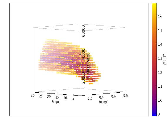
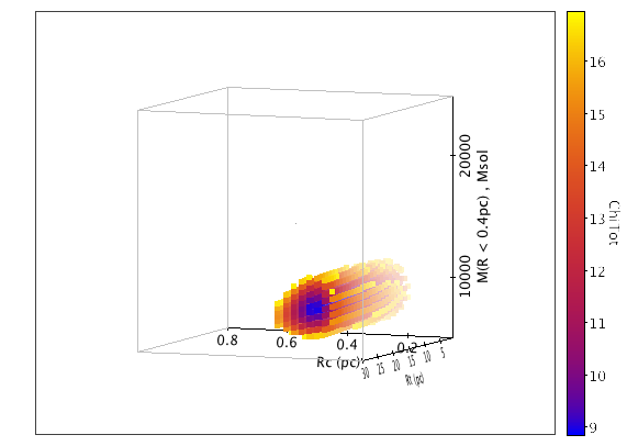
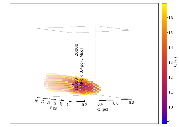
We vary the parameters of the King model (core radius $R_{c}$, tidal radius $R_{t}$ and total cluster mass $M_{cl}$) and map the variation of $\chi^{2}$ when the projected dispersion profile is compared with that obtained from observation. With three model parameters varying we adopt $\Delta\chi^{2}=3.50,~{}7.82~{}\&~{}13.93$, which correspond to 68%, 95% and 99.7% of probability ($``1\sigma^{\prime\prime}$, $``2\sigma^{\prime\prime}$ & $``3\sigma^{\prime\prime}$) when three model parameters are allowed to jointly vary (see, for example, Press et al. 2002). The limits on quantities derived from these parameters are then given by the range of values of the derived parameters within each $\Delta\chi^{2}$ region of interest.

Our proper motion data do not by themselves constrain the shape of the cluster, as they are concentrated in its innermost regions (for example, our data fall entirely within the estimated $R_{hm}\approx 0.4$ pc of Stolte et al. 2005). We therefore incorporate surface density data $\Sigma_{N}(R)$ (units stars pc^-2) from the literature. We have proper motion constraints from five radial annuli; comparison of these data alone to the velocity dispersion model yields the figure of merit $\chi^{2}_{\rm kinem}$. Comparison of the seven radial estimates of $\Sigma_{N}(R)$ from Espinoza et al. (2009) to model prediction then yields the figure of merit $\chi^{2}_{full}$. The full figure of merit is then

$$\chi^{2}_{kinem} \equiv \chi^{2}_{R}+\chi^{2}_{T}$$

$$= \sum^{5}_{i=1}\frac{\left[\sigma_{R}({\rm data})-\sigma_{R}(\rm model)\right]^{2}_{i}}{\Delta^{2}_{R,i}}+\sum^{5}_{i=1}\frac{\left[\sigma_{T}({\rm data})-\sigma_{T}(\rm model)\right]^{2}_{i}}{\Delta^{2}_{T,i}}$$

$$\chi^{2}_{full} \equiv \chi^{2}_{R}+\chi^{2}_{T}+\chi^{2}_{\Sigma}$$ (8)

$$= \chi^{2}_{kinem}+\sum^{7}_{i=1}\frac{\left[\Sigma_{N}({\rm data})-\Sigma_{N}(\rm model)\right]^{2}_{i}}{\Delta^{2}_{\Sigma,i}}$$

where $\Delta^{2}$ represent the squared errors on each datapoint.

Since the cluster is in reality mass segregated (e.g. Figer et al. 1999; Stolte et al. 2005), the underlying mass distribution that dominates the velocity dispersion is unlikely to be more centrally concentrated than the massive stars directly amenable to observation. Espinoza et al. (2009) assess $\Sigma_{N}(R)$ for massive stars in different mass ranges; we report here the mass limits using the least centrally-concentrated massive-star sample ($10\leq M_{\ast}/M_{\odot}\leq 30$) of Espinoza et al. (2009). Fitted parameters and the behavior of the $\chi^{2}$ surface for different choices of $\Sigma_{N}(R)$ (as well as no constraint on $\Sigma_{N}(R)$, i.e., fitting with kinematic data only) are discussed in Appendix E.

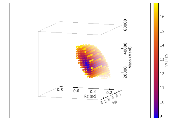
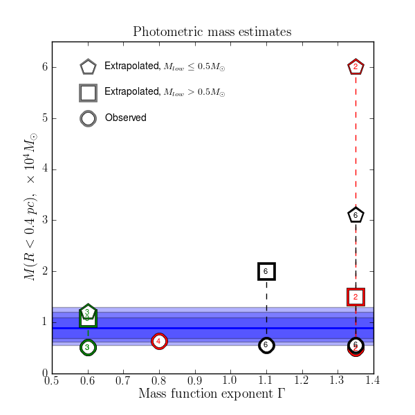
Figure 8 shows the behaviour of $\chi^{2}$ as the model parameters $R_{c},R_{t},M_{cl}$ are varied, incuding the $\Sigma_{N}(R)$ sample just discussed. Figure 9 illustrates the variation of $\chi^{2}_{full}$ aganst $R_{c},R_{t},M(R<0.4~{}{\rm pc})$. Figure 10 shows radial profiles drawn from within the $\Delta\chi^{2}_{full}=7.82$ surface in parameter space, which corresponds to 95$\%$ formal significance (or 2$\sigma$). As can be seen, a wide range of $M(r<1.0~{}{\rm pc})$  is consistent with the kinematic and surface-density data, but a rather narrow range of $M(R<0.4~{}{\rm pc})$  is consistent with the flat plateau and magnitude of the velocity dispersions we measure. Specifically, we find $M(R<0.4~{}{\rm pc})=0.90^{+0.40}_{-0.35}\times 10^{4}M_{\odot}$, $M(r<1.0~{}{\rm pc})=1.5^{+0.74}_{-0.60}\times 10^{4}M_{\odot}$ and $M_{cl}=3.16^{+2.46}_{-2.09}\times 10^{4}M_{\odot}$.

All isotropic models tested yield an upper limit on $M(R<0.4~{}{\rm pc})$  of $1.30\times 10^{4}~{}M_{\odot}$ at formal $3\sigma$ confidence (Appendix E). Inclusion of $\Sigma_{N}(R)$ removes the very low estimates of $M(R<0.4~{}{\rm pc})$  from consideration, with the largest lower limit obtained using the full mass range of Espinoza et al. 2009). With the most massive stars included in $\Sigma_{N}(R)$, core radii $R_{c}<0.13$ pc are rejected at the 3$\sigma$ level; this level is well above the minimum grid value of $R_{c}=0.05$ pc. Therefore the grid boundaries are not leading us to assume an artificially compact cluster. The total cluster mass is only very weakly constrained from kinematic data alone.

We also attempted to account for a wide range of cluster anisotropies using the algorithm of LM89. This method differs from the “forward” modeling we describe here, in that the isotropic velocity dispersion profile is modified for anisotropy, the enclosed mass $M(<r)$ estimated from the full Jeans equation using this dispersion profile, and the density profile $\rho(r)$ estimated from the form of $M(<r)$. While we were unsuccessful in reproducing the LM89 approach for a King (1962) profile, parameterization of the cluster with a Plummer profile and allowing for anisotropy (following Leonard et al. 1992) was more fruitful. This yielded a slightly wider range of compatible values of $M(R<0.4~{}{\rm pc})$ , though still below 1.5$\times 10^{4}~{}M_{\odot}$ at the formal $2\sigma$ confidence level. Appendix E outlines the mass modeling using anisotropic cluster models following the method of Leonard & Merritt (1992); mass limits so produced do not alter the conclusions of this report.

5.2 Comparison to literature mass estimates

Unlike photometric mass estimates, which rely heavily on an accurate completeness and extinction correction to map the observed population onto the underlying population, a kinematic mass estimate only requires that the motion of a selection of tracer objects be well-measured (and of course that the assumptions in the mass modeling be reasonable). We compare our mass estimates with literature estimates here.

5.2.1 Literature mass estimates

With the exeption of the radial-velocity kinematic estimate of Figer et al. (2002), all observational mass estimates of the Arches cluster refer to the projected mass within some radius on the sky, i.e., $M(<R)$. Since this is also the best-constrained of our kinematic mass estimates, we focus our literature discussion on these estimates.

Serabyn et al. (1998) extrapolated the mass estimated from observed O-stars down to low masses to estimate the cluster stellar mass; they used $JHK^{\prime}$ imaging with NIRC on Keck-I to estimate a total of $5,000\pm 1000~{}M_{\odot}$ in $100\pm 50$ massive O-stars in the cluster, which they extrapolated to the full range of stellar masses using a mass function exponent $\Gamma=1.35$. This yielded  $M_{cl}(R<0.35~{}{\rm pc})=(1.5,6)\times 10^{4}M_{\odot}$, for lower stellar-mass limits (2,0.1) $M_{\odot}$ respectively.

Figer et al. (1999) used $NICMOS$ on $HST$ to perform a photometric census down to a photometric limit corresponding to about $6M_{\odot}$. Within an annulus $0.12\leq R<0.37~{}pc$ they measured about $0.51\times 10^{4}M_{\odot}$ in stars, which, using the PDMF measured for the same stars, was extrapolated to a total mass for this outer annulus. The number counts of bright stars were then used to estimate the scale factor from the outer annulus ($0.12\leq R<0.37$ pc) to the entire inner cluster ($R<0.37$ pc), yielding a total mass of the inner cluster $M_{cl}(R<0.37~{}{\rm pc})=(1.08-1.20)\times 10^{4}M_{\odot}$ depending on the lower mass cutoff adopted (1.0 - 0.1) $M_{\odot}$, and a top-heavy PDMF exponent ($\Gamma\approx 0.6$).

Stolte et al. (2002) used Gemini NGS/AO photometry and the HST/NICMOS data of Figer et al. (1999) to search for variation of $\Gamma$ with projected radius from the cluster center, using Geneva isochrones (Lejeune & Schaerer, 2001) to convert from magnitude to mass. They obtained a half-mass radius $R_{hm}=10^{\prime\prime}=0.4$ pc. By summing the observed mass histogram in two projected-radial bins within $R_{hm}$, they estimated a total mass amongst the stars measured, of $0.63\times 10^{4}M_{\odot}$. The authors preferred not to extrapolate the mass function beneath their photometric limit of about $2M_{\odot}$ due to the uncertainties in so doing. They pointed out also that their estimate is not corrected for incompleteness, and so their estimate for the total mass within $r_{hm}$ is therefore $M_{cl}(<0.4~{}{\rm pc})\sim 10^{4}M_{\odot}$. Note that this is the total stellar mass within a cylinder of radius $R=10^{\prime\prime}\equiv 0.4$ pc at $\sim$8 kpc, not the total stellar mass in the cluster. Stolte et al. (2002) found a PDMF exponent $\Gamma\sim 0.8\pm 0.2$ as a spatial average, but with considerable spatial variation as a function of projected radius, though this does not affect their mass estimate. At $R<5^{\prime\prime}$ the PDMF is nearly flat, developing to $\Gamma=1.04\pm 0.29$ at $5^{\prime\prime}<R<9^{\prime\prime}$ and consistent with Salpeter at greater radii ($\Gamma=1.69\pm 0.66$ for $10^{\prime\prime}<R<20^{\prime\prime}$).

Espinoza et al. (2009) report the use of VLT/NACO photometry to fit mass function exponents for two annuli in projected radius; $R<0.2$ pc and $0.2<R<0.4$ pc. Differential reddening-corrections on a star-by-star basis were used. The authors prefer to quote the initial masses from Geneva isochrones rather than present-day masses, and therefore give the initial mass function exponents $\Gamma_{0}$; they find a spatially-averaged $\Gamma_{0}=1.1\pm 0.2$ for $M>10M_{\odot}$, consistent with Salpeter, and point out that this index is about 0.1-0.15 dex steeper than PDMF indices reported in the literature. Integrating the IMF down to a low-mass cut-off of $1M_{\odot}$, Espinoza et al. (2009) report $M_{cl}(R<0.4)~{}{\rm pc}=(2\pm 0.6)\times 10^{4}M_{\odot}$. Whether a low-mass truncation exists at all in the Arches mass function is an open question; Espinoza et al. (2009) therefore use a Kroupa (2002) mass function to estimate $M_{cl}(R<0.4~{}{\rm pc})=(3.1\pm 0.6)\times 10^{4}M_{\odot}$ without a lower-mass cut-off. While the extrapolation to total cluster mass depends on the radial dependence of the PDMF and the density profile, N-body models suggest (Harfst et al., 2010) that roughly half the cluster mass is observed between projected radius $R=0.4$ pc and the tidal radius $\sim 1$ pc, which would suggest that the total present-day cluster mass indicated by Espinoza et al. (2009) is closer to $M_{cl}=(4\pm 1.2)\times 10^{4}M_{\odot}$ and $M_{cl}=(6.2\pm 1.2)\times 10^{4}M_{\odot}$ for lower mass limits of $1.0M_{\odot}$ and $0.08M_{\odot}$, respectively.

5.2.2 Additional mass estimates

In addition to photometric mass estimates discussed above, the Arches total mass is often used as input to models of the formation and evolution of massive clusters. To better place our work in context, all reported mass estimates for the Arches of which we are aware have been collated into Table 10. Most of the total initial mass estimates used in Fokker-Planck (e.g. Kim et al. 1999) and N-body simulations (e.g., Kim et al., 2000; Portegies Zwart et al., 2002b; Harfst et al., 2010) lie in the range $M_{0}\sim 1-5\times 10^{4}M_{\odot}$. However there are some notable outliers; in particular, work approaching the Arches formation from the point of view of cloud fragmentation (generating the IMF) assumes a very high initial cluster mass (e.g. $M_{0}\sim 15\times 10^{4}M_{\odot}$ Dib, 2007). The connection between initial cluster mass for models and observed present day mass depends on a number of complicated factors that render direct comparison of $M_{0}$ to observation highly assumption dependent; the Arches has probably lost roughly half of its stellar mass since formation (e.g. Kim et al., 2000; Harfst et al., 2010).

5.2.3 Proper motion-derived mass estimate compared to literature mass estimates

Isotropic King (1962) profiles produce estimates of the present-day projected mass $M(R<0.4~{}{\rm pc})$  that are at least $3\sigma$ below the $M(R<0.4~{}{\rm pc})$ = $(3.1\pm 0.6)\times 10^{4}~{}M_{\odot}$ derived by Espinoza et al. (2009) under the assumption of a non-top-heavy mass function and no lower-mass truncation. In contrast, photometric estimates assuming either a low-mass truncation or top-heavy mass function, or both, are more compatible with our dispersion data under the assumptions of our mass models. In particular, our upper limit of $1.30\times 10^{4}M_{\odot}$ from isotropic King modeling is 1.5$\sigma$ below the photometric estimate of Espinoza et al. (2009) with a lower-mass cut-off at 1$M_{\odot}$ using a mass function that is not strongly top-heavy. In addition, the mass ranges of Figer et al. (1999) are highly compatible with our dispersion-based mass estimate.

Within the limitations of our modeling, then, our velocity dispersion estimate is compatible with a mass function that is either top-heavy, truncated at low-mass, or both. A Salpeter PDMF without low-mass truncation is not indicated by our data.

We remind the reader that our mass limit is a first estimate with a straightforward model, which is likely subject to update when the full machinery of simulation is brought to bear on the problem using our dispersions as a constraint. On the modeling side, several factors complicate the interpretation of velocity dispersion data. Firstly, the location of the Arches cluster in a strong tidal field suggests the assumptions of spherical symmetry and negligible rotation may be violated. Secondly, while the degree of mass segregation in a young post-collapse cluster is different for stars of different masses, after $\sim 2$ Myr, the massive stars whose motion we measure ($M\gtrsim 10M_{\odot}$) are likely to have undergone some mass segregation (Allison et al., 2009). Therefore we are measuring tracer stars whose velocity dispersion may be biased to low values. Velocity dispersions constructed from proper motion observations of stars solely with masses $M\lesssim 10M_{\odot}$ (i.e., $K^{\prime}\gtrsim 16$) would provide a second mass estimate from a population less sensitive to mass segregation (see Figure 2 of Allison et al., 2009). For the present dataset this sample is almost entirely on the steeply-rising part of the error-magnitude curve (Figure 2). Investigation of this sample is outside the scope of the present communication. At the present stage of our investigations, we limit ourselves to pointing out that our mass estimate may be biased to low values by our sample selection of massive stars that have likely undergone some degree of dynamical mass segregation.

On the observational side, we do not yet have sufficiently precise motions outside 0.2pc to constrain M(R) outside this region, and have had to resort to projection of models that have significant caveats when applied to this cluster. Future observations of the outer fields should remedy this situation.

Note that, unlike with radial-velocity studies, binaries are unlikely to have an effect on the velocity dispersion measurement we report here. To produce an effect of the same order of magnitude as the proper motion dispersion we obtain, a substantial binary population would be needed in which the binary orbit shifted the center of near-IR light by $\sim 0.3$ mas over the three-year timebase of our observations. A binary with components $150~{}\&~{}50~{}M_{\odot}$ in a 1,000d orbit would exhibit semimajor axis and orbital speed of adequate magnitude ($a\simeq 0.36$ mas, $v\simeq 0.13$ mas yr^-1, respectively) to produce this effect (assuming the near-IR brightness ratio corresponding to this mass ratio is sufficient for the center of light to move). However, we expect such systems to be too rare to produce any effect on the dispersion measurement over the Arches population. Furthermore, such systems would be confined to the brightest magnitude-bin in our analysis, leading to a decrease in measured dispersion with increasing apparent magnitude, which is not observed. Appealing to high eccentricity introduces an additional selection-effect (on the orientation of the orbit to produce measurable motion). Thus we conclude binaries are an insignificant contributor to the measured velocity dispersion in the Arches cluster (compare with Gieles et al. 2010).

5.3 Mean motion of the cluster

The 2D Gaussian profile of the field component in the VPD shows an axis ratio that is roughly constant with magnitude, while its contribution to the sample in the field of view increases as fainter objects are probed. Its orientation in the VPD is consistent with the galactic plane, indicating that the velocity dispersion along the field major-axis in the VPD is strongly affected by differential rotation.

The bulk motion of the Arches with respect to the field population is 172 $\pm$ 15 km s^-1 (the inverse variance-weighted average of the $14<K<16$ and $16<K<18$ bins). Including the $18<K<20$ bin revises this figure downward to 153 $\pm$ 11 km s^-1; however in this magnitude range the proper motion error curve rises steeply with magnitude (Figure 5), so objects this faint may be particularly vulnerable to misclassification bias (Appendix D). This is slightly smaller than the $212\pm 29$ km s^-1 determined previously (Stolte et al., 2008). This is probably due to two competing biases in the previous work that oppose each other: Stolte et al. (2008) imposed a hard membership limit, where all objects within a certain velocity from the cluster center in the VPD are denoted cluster objects, which tends to exaggerate the cluster-field separation in the VPD by cutting off one side of the field component. Conversely, they included objects at all magnitudes in their estimate of the bulk motion, which tends to reduce the estimated component separation (see Appendix D).

In their study of the Arches bulk motion, Stolte et al. (2008) found that, although the Arches is unlikely to be on a circular orbit, integration of its path through the potential of the inner Milky Way indicated the cluster was unlikely to pass sufficiently close to the GC to spiral in towards it and donate its stars to the GC nuclear cluster. Our revised motion estimate makes the Arches orbit slightly more compatible with circular motion. Following the arguments of Stolte et al. (2008), if on a circular orbit, ${\bf v.r}=0$ then demands an enclosed mass only $1.5\sigma$ above that measured photometrically (Launhardt et al., 2002). At first glance, our new bulk motion supports the conclusions of Stolte et al. (2008) that a cluster that is dynamically similar to the Arches is unlikely to be a future source of young stars for the GC star cluster. Integration of the Arches motion through the potential of the inner Milky Way using our new motion determination is required to draw further conclusions about the formation and subsequent motion of the cluster.

Interpretation of the cluster bulk motion is complicated by three factors. First, the kinematic parameters of the field component depends on the distribution of tracer stars along the line of sight as well as their motion. Differential rotation by field stars participating in Galactic rotation may therefore vary with tracer-star brightness (with observations to different depths picking up different field-tracer populations). Second, the field population (or a significant component of the field population) may show its own motion beyond galactic rotation; for example this motion may be dominated by bar rotation on the nearside of the GC (if the far side of the bar suffers from higher extinction). Or, rotation of the NSD could impose a mean motion of the field component with respect to the Arches cluster. Third, extinction variations along the line of sight coupled with the low-number statistics ($\sim$ few tens of field objects in each magnitude bin; Table 6) may reduce the validity of a gaussian to represent the field component in the first place. Thus our quoted error of $15$ km s^-1 on the Arches bulk motion is likely an underestimate. Stolte et al. (2008) discuss further some of the difficulties associated with interpreting a bulk motion against a mean-field population.

5.4 Properties of the field population

Within the measurement errors, the orientation of the field ellipse is entirely consistent with the direction of the vector joining the cluster and field centers in the VPD, indicating the Arches moves along the direction of preferential motion for the field (Table 6).

To our knowledge, the covariance ${\bf Z}_{k}$ of the field component provides the first estimate of the stellar velocity dispersion of the bulge along such a close sight-line to the Galactic center. This will allow a direct constraint on the bulge potential along this sight-line, which itself is a key ingredient in the use of cluster bulk motion to assess its likely path through the inner Milky Way (Stolte et al. 2008). Here we restrict ourselves to a comparison of ${\bf Z}_{k}$ with the velocity dispersion of the Bulge at higher latitudes.

The bulge is a highly complex stellar structure, with many basic parameters presently under debate, complicated by shifting nomenclature in the literature. Several components appear to be present, with the relationship between them still far from settled. Chemical evidence suggests most of the stars formed early and rapidly, as might be expected for a “classical” bulge component (e.g., McWilliam & Rich, 1994; Lecureur et al., 2007), while the spatial arrangement and motion of the stars suggests a bar structure, driving a “boxy/peanut” bulge (e.g., Dwek et al., 1995; Howard et al., 2009; McWilliam & Zoccali, 2010; Shen et al., 2010).

Whatever its formation history, the present-day bulge shows variation of stellar kinematics with metallicity. Soto et al. (2007) report variation of the shape of the $\sigma_{r},\sigma_{l}$ velocity ellipsoid with metallicity (Zhao et al. 1994 provide an early detection of vertex deviation in the bulge). Babusiaux et al. (2010) present proper motion dispersions as a function of metallicity for the Baade’s Window (hereafter, BW) field ($l=0\arcdeg,b=-0.4\arcdeg$), significantly farther out from the GC than our sample. For stars of approximately solar and higher metallicity, they report $\sigma_{l},\sigma_{b}=107\pm 6,94\pm 6$ km s^-1. For stars with $[Fe/H]<-0.14$, Babusiaux et al. (2010) report $\sigma_{l},\sigma_{b}=138\pm 12,103\pm 7$ km s^-1.

To estimate the velocity dispersion of the Arches field component we take the variance-weighted mean of the determinations from the three non-overlapping bins ($14.0\leq K^{\prime}<16.0$; $16.0\leq K^{\prime}<18.0$ and $18.0\leq K^{\prime}<20.0$). This yields major-axis and minor-axis dispersions of $\overline{\sigma_{a,f}}=2.72\pm 0.15$ mas yr^-1 and $\overline{\sigma_{b,f}}=1.69\pm 0.10$ mas yr^-1, which scale to the distance of the Galactic center ($8.4\pm 0.4~{}{\rm kpc}$; Ghez et al. 2008) as $103\pm 7.7$ km s^-1 and $64\pm 5.0$ km s^-1. The orientation of the field component in the vector point diagram (VPD), expressed as a position-angle East of North, is $\overline{\theta_{f}}=+30.5\arcdeg\pm 7.1\arcdeg$ (motion along the galactic plane corresponds to about $+27.1\arcdeg$ in the VPD). For the remainder of this section we therefore identify the field velocity dispersion major axis with the galactic plane, so $\sigma_{a,f},\sigma_{b,f}$ represent the field velocity dispersion in galactic longitude and latitude respectively. Thus our field velocity dispersion is more consistent with the higher-metallicity BW stars, which is currently interpreted by Babusiaux et al. (2010) as a bar-dominated population.

Some caution is warranted interpreting ${\bf Z}_{k}$ for the field, as a number of parameters of the field population are still not fully understood. First, the NSD imprints its own motion on the field, which may be coherent and different from the motion of the bulge/bar system. Second, the mass distribution of the composite bulge along our line of sight is not fully constrained; for example the range in bar orientation estimates in the galactic plane still ranges by $45\arcdeg$ (Benjamin et al., 2005; Robin et al., 2009; McWilliam & Zoccali, 2010, e.g.,). Third, astrometric completeness likely biases the bulge motion we observe towards the near-side of the GC, so the field motion is sampled at some preferred mean distance from the GC. Fourth, the mixture of bulge and bar components making up the field population is not yet fully constrained.

5.5 Membership probabilities and $L^{\prime}$-excess sources

Our refined membership probabilities allow a clean-cluster sample to be extracted for further work. Appendix F lists the formal membership probabilities (equation 2) for well-measured stars in our sample. The use of this cleaned sample to probe the cluster mass function is underway by our group (McCrady et al., 2011), and will be reported in a following communication. For now, we note that the Keck-Keck motions provide support to the conclusions of Stolte et al. (2010), that a significant number of stars with circumstellar disks are likely present in the Arches cluster. These stars appear redward of the locus of most stars in the Arches in the $H-K$ color-magnitude diagram; since $L^{\prime}$-excess sources cannot be distinguished from field stars based on $H-K^{\prime}$ color alone, kinematic separation is essential. Of sixteen objects falling within the locus of points redward of the cluster main sequence within the CMD (Figure 7, six show proper motions suggestive of cluster membership. More generally, however, we find that most of the outliers from the main locus of Arches stars in the $H-K$ CMD are indeed kinematically associated with the field.

6 Conclusions

With uniform observational setup over a sufficient time baseline and careful accounting for a number of sources of proper motion error, we have measured the internal velocity dispersion of the Arches cluster for the first time, finding $\sigma=0.15\pm 0.01$ mas yr^-1, which corresponds to $5.4\pm 0.4$ km s^-1 at a distance of 8.4 kpc.

We have used this dispersion to test the photometric estimates of the present-day mass function (PDMF) of the Arches cluster. The total mass is likely in the range $M(r<1.0~{}{\rm pc})=1.5^{+0.74}_{-0.60}\times 10^{4}M_{\odot}$, but this is only weakly constrained by kinematic data and is consistent with nearly all suggestions of total cluster mass from the modeling literature. The projected mass (i.e., mass contained within a cylinder of radius $R$ on the sky) is rather better constrained; we find $M(R<0.4~{}{\rm pc})=0.90^{+0.40}_{-0.35}\times 10^{4}M_{\odot}$ at formal $3\sigma$ confidence. The upper bound of this range is $3\sigma$ below the photometric estimate for $M(R<0.4~{}{\rm pc})$  estimated by Espinoza et al. (2009) under the assumptions of a non-top-heavy mass function without low-mass truncation. If a substantial contribution from massive binaries were unknowingly included in our measurement, this would strengthen our conclusion because the upper cluster mass bound would accordingly be reduced. This is the first mass estimate for the Arches based on proper motion velocity-dispersion.

We have also revised the bulk motion of the Arches slightly downward. Our updated motion of $172\pm 15$ km s^-1 is only slightly lower than the $212\pm 29$ km s^-1 determined previously (Stolte et al. 2008). Taken at face value, this supports the previous conclusion that the Arches Cluster is unlikely to pass within 10 pc of the GC.

Finally, we have provided the first estimate (to our knowledge) of the velocity dispersion of the Bulge along such a close sight-line to the Galactic center; this estimate is (103, 64) $\pm$ (7.7,5.0) km s^-1, with the major axis coincident with the Galactic plane, to within the uncertainties.

Figure 1: NIRC2 $K^{\prime}$ mosaic of the core field of the Arches in May 2009. This is our best map in terms of both resolution (51 mas) and sensitivity ($K^{\prime}_{lim}=20.59$ mag; Table 1). All stars on which we report in this paper fall within the field of view indicated here. The scale-bar is two arcseconds in length. Stars used as PSF reference-stars are indicated by circles. When stellar membership probabilities are reported, positions are reported as offsets from the reference star indicated by the square in this figure.

Figure 2: Positional errors as measured for an example epoch (2008.50). Positions are those in the image-stack with centroiding errors assessed as the rms of measurements within an epoch (Section 3.3.1). Top row: centroiding errors along detector-X and detector-Y (top-left and top-middle respectively), and the average of the two as a function of distance from the field center (top-right). Bottom row: alignment errors along X and Y (bottom-left and bottom-middle; Section 3.3.2). The magnitude histogram is given in the bottom-right panel.

Figure 3: Five example positional time-series. Left columns show motion along X, right columns along Y. Object IDs and $K^{\prime}$ magnitudes are indicated in the right top and bottom corners respectively. Note that each vertical axis is scaled to accommodate the motion of the star and is in units of pixels in the $t_{ref}$  reference frame. The best-fit straight line to the motions are indicated in each case, as are 1$\sigma$ positional error curves. Object 154 is likely a field object, as indicated by its large proper motion relative to the reference frame.

Figure 4: The distribution of adopted proper motion precision (Section 3.3 and Table 4), for all objects with five position-measurements. Outliers due to likely mismatches are indicated by squares and were removed from the analysis. An object qualifies as an outlier if the rms in either co-ordinate falls obviously outside the sequence defined by most of the points.

Figure 5: Vector Point Diagrams for the overlapping magnitude-ranges of Section 4.1.1 and Table 6. Shaded ellipses give the $1\sigma$ contours for the two-dimensional gaussian components fit to the field and cluster components. Within each ellipse, the lines indicate the length and direction of the semimajor (thick red line) and semiminor (thin red line) axes.

Figure 6: Observed velocity dispersion in each coordinate for stars with $14.0\leq K^{\prime}<17.0$ compared to a gaussian of width equal to the mean measurement error over this range (Section 3.3 and Table 4). Panels correspond to detector-X (Top) and detector-Y (bottom). This figure was constructed after removing likely field objects (Section 4.1)

Figure 7: Color-magnitude diagram (CMD) and Vector Point Diagram (VPD) for all objects with proper motion error $<0.5$ mas yr^-1 and five epochs of measurement. The CMD presented here was constructed by matching $K^{\prime}$ measurements to photometry taken in $H$-band in 2006 May with Keck-2/NIRC2-LGS (McCrady et al., 2011), which limits the depth in the CMD. Objects with $P_{\rm{cluster}}>0.995$ are shown in black, all other objects denoted with open circles. Red objects in the VPD correspond to the stars within the red dot-dashed box in the CMD, and represent well-measured objects with a possible $H-K^{\prime}$ excess. Of these objects, those with $P_{\rm cluster}>0.995$ are shown with a red circle; their field counterparts are shown with red squares. See Section 5.5 and Stolte et al. (2010) for more information on these objects.

Figure 8: Views of the $\Delta\chi^{2}_{full}<7.82$ region when both kinematic and surface density data (for stars of mass $10\leq M/M_{\odot}\leq 30$; Espinoza et al. 2009) are included in the assessment. Axes are: $R_{c},R_{t},M_{cl}$, with total cluster mass $M_{cl}$ vertical in each case. Limits shown are: $0.05\leq R_{c}\leq 0.8$ pc; $1.0\leq R_{t}\leq 30$ pc; $0.5\leq M_{cl}\leq 6.0\times 10^{4}M_{\odot}$.

Figure 9: As Figure 8, but with $M(R<0.4~{}{\rm pc})$  along the vertical axis. Limits shown are: $0.05\leq R_{c}\leq 0.8$ pc; $1.0\leq R_{t}\leq 30$ pc; $0.5\leq M(R<0.4~{}{\rm pc})\leq 2.5\times 10^{4}M_{\odot}$.

Figure 10: Radial profiles corresponding to parameter-sets within the $\Delta\chi^{2}_{full}<7.82$ surface; both our own kinematic data and surface density (by number) $\Sigma_{N}(R)$ data are used (corresponding to stars of mass $10\leq M/M_{\odot}\leq 30$; Espinoza et al. 2009). Top-left and top-middle panels show radial and tangential velocity dispersions from proper motions (points) over the projected profiles corresponding to model parameters (lines). Top-right panel shows the $\Sigma_{N}(R)$ dataset with model predictions. Bottom-left and bottom-middle panels show the total mass within cylindrical radius $R$ on the sky, with $R=0.4$ pc indicated by the vertical dashed line. Bottom-right panel shows the mass enclosed within a sphere of radius $r$ pc from the cluster center. See also Table 9.

Figure 11: Photometric mass estimates for the Arches cluster from the literature. Symbols give the directly-observed photometric mass (circles) and extrapolated mass (where reported; squares and pentagons) depending on the low-mass cut-off assumed. The citation for each estimate is shown inside the symbols (using the numbering of Table 10). The horizontal bands show our model-dependent mass estimate using our dispersion data (at 1$\sigma$, 2$\sigma$ and 3$\sigma$), and the $\Sigma_{N}(R)$ dataset of Espinoza et al. (2009); see Section 5.1 for more detail on the mass modeling used. All masses are reported as $M(R<0.4~{}{\rm pc})$ .

Epoch	(t${}_{int}\times N_{coadd}$)	$N_{images}$	$N_{use}$	FWHM	Strehl	$N_{\ast}$	$N_{\ast,{\rm uncrowd}}$	$K^{\prime}_{lim}$
	(s)			(mas)				(mag)
2006 May 21	3.00 $\times$ 10	15	15	61.05	0.261	660	649	19.43
2006 Jul 18	3.00 $\times$ 10	52	38	56.95	0.349	657	642	19.89
2008 May 13	3.00 $\times$ 10	146	72	66.66	0.219	556	536	19.74
2008 Jun 01	3.00 $\times$ 10	89	83	54.96	0.373	845	810	20.42
2009 May 02	2.80 $\times$ 10	119	108	51.47	0.442	968	917	20.59

Table 1: Summary of observations. Reading left-right, the columns are: Epoch of observation, the total integration time for each image, the number of images observed, the number of images used, the median FWHM and Strehl ratio over the set of accepted images $N_{use}$, the number of stars measured within the mean image stack in each epoch; the number surviving the cut on proximity to a known neighbour, and finally the magnitude $K^{\prime}_{lim}$ at which the cumulative distribution function of the observed $K^{\prime}$ magnitudes reaches 90$\%$ of the total number of stars in the sample at each epoch.

Table 2: PSF stars. Reading left-right, columns are: sequential star number in the master table of membership probabilities, estimated brightness, and finally the position of the star expressed as an offset in arcseconds from the reference star along the (E-W) and (S-N) directions. See Figure 1 for the locations of these stars on the field of view.

Row	$K^{\prime}$	$\Delta x$	$\Delta y$
	(mag)	($"$)	($"$)
1	10.24	2.736	-3.943
2	10.48	2.063	-1.193
3	10.49	0.791	0.755
4	10.66	3.150	-2.899
5	11.08	-0.633	-4.252
7	11.22	-1.650	1.730
8	11.25	1.385	-2.334
16	12.18	1.012	-5.199
24	12.49	0	0
25	12.50	5.407	-0.218
32	12.88	2.499	-5.402

Parameter		2006.38	2006.54	2008.37	2008.50	2009.33
$N_{ref}$		238	239	235	241	233
$N_{<4}$		9	10	21	11	6
$\Delta$	$x^{\prime}$	-83.94 $\pm$ $6.03\times 10^{-3}$	9.26 $\pm$ $4.01\times 10^{-3}$	4.16 $\pm$ $3.71\times 10^{-3}$	(-4.06 $\pm$ 17.716)$\times 10^{-4}$	6.53 $\pm$ $3.52\times 10^{-3}$
(pix)	$y^{\prime}$	-16.88 $\pm$ $4.74\times 10^{-3}$	5.69 $\pm$ $4.39\times 10^{-3}$	3.35 $\pm$ $5.64\times 10^{-3}$	(3.66 $\pm$ 25.421)$\times 10^{-4}$	3.51 $\pm$ $3.66\times 10^{-3}$
$x$	$x^{\prime}$	1.00005 $\pm$ $2.11\times 10^{-5}$	0.99994 $\pm$ $9.12\times 10^{-6}$	1.00025 $\pm$ $1.34\times 10^{-5}$	0.99999 $\pm$ $6.18\times 10^{-6}$	1.00002 $\pm$ $8.24\times 10^{-6}$
()	$y^{\prime}$	(6.64 $\pm$ 0.185)$\times 10^{-4}$	(7.73 $\pm$ 0.079)$\times 10^{-4}$	(1.33 $\pm$ 1.425)$\times 10^{-5}$	(2.32 $\pm$ 5.858)$\times 10^{-6}$	(2.75 $\pm$ 0.090)$\times 10^{-4}$
$y$	$x^{\prime}$	(-3.15 $\pm$ 0.177)$\times 10^{-4}$	(-3.53 $\pm$ 0.089)$\times 10^{-4}$	(1.23 $\pm$ 0.105)$\times 10^{-4}$	(-2.40 $\pm$ 4.766)$\times 10^{-6}$	(-2.54 $\pm$ 0.072)$\times 10^{-4}$
()	$y^{\prime}$	1.00046 $\pm$ $1.97\times 10^{-5}$	1.00028 $\pm$ $9.62\times 10^{-6}$	1.00014 $\pm$ $1.34\times 10^{-5}$	1.00000 $\pm$ $6.66\times 10^{-6}$	1.00009 $\pm$ $7.99\times 10^{-6}$
$x^{2}$	$x^{\prime}$	28.90 $\pm$ 5.946	20.61 $\pm$ 3.463	-18.24 $\pm$ 3.989	-0.27 $\pm$ 1.986	4.63 $\pm$ 2.818
($\times 10^{-8}$ pix-1)	$y^{\prime}$	11.78 $\pm$ 4.751	15.66 $\pm$ 3.266	23.10 $\pm$ 4.404	0.48 $\pm$ 1.937	20.65 $\pm$ 2.938
$xy$	$x^{\prime}$	1.80 $\pm$ 5.818	20.39 $\pm$ 3.772	58.96 $\pm$ 4.594	-0.28 $\pm$ 2.040	-0.58 $\pm$ 2.973
($\times 10^{-8}$ pix-1)	$y^{\prime}$	-5.05 $\pm$ 6.935	-10.19 $\pm$ 3.985	-28.61 $\pm$ 5.203	-1.52 $\pm$ 2.680	-20.03 $\pm$ 3.335
$y^{2}$	$x^{\prime}$	-3.04 $\pm$ 5.917	5.55 $\pm$ 3.048	1.09 $\pm$ 3.540	1.71 $\pm$ 1.686	-0.59 $\pm$ 2.959
($\times 10^{-8}$ pix-1)	$y^{\prime}$	33.22 $\pm$ 6.228	52.07 $\pm$ 3.664	75.11 $\pm$ 5.451	-1.13 $\pm$ 2.488	-0.47 $\pm$ 2.633
$1.0$-$M$		-2.55 $\pm$ 0.150	-1.14 $\pm$ 0.064	-1.95 $\pm$ 0.095	(1.97 $\pm$ 4.303)$\times 10^{-2}$	-0.58 $\pm$ 0.062
($\times 10^{-4}$ )
$1.0$-$M_{y}/M_{x}$		-4.08 $\pm$ 0.275	-3.34 $\pm$ 0.135	1.10 $\pm$ 0.189	(-5.72 $\pm$ 9.564)$\times 10^{-2}$	-0.71 $\pm$ 0.104
($\times 10^{-4}$ )
$\theta_{rot}$		-10.11 $\pm$ 0.250	-11.62 $\pm$ 0.129	1.13 $\pm$ 0.182	(-4.88 $\pm$ 7.925)$\times 10^{-2}$	-5.46 $\pm$ 0.116
(′′)
$\theta_{skew}$		7.20 $\pm$ 0.553	8.66 $\pm$ 0.234	2.82 $\pm$ 0.364	-0.002 $\pm$ 0.153	0.43 $\pm$ 0.245
(′′)

Table 3: Transformation parameters taking the starlist in each epoch into the reference frame $t_{ref}$. Top row: Number of reference stars $N_{ref}$ used in the mapping, along with the number of reference stars $N_{<4}$ that appear in fewer than four epochs. Next six rows: Coefficients of the polynomial fits $x^{\prime}=f(x,y)$ and $y^{\prime}=g(x,y)$ (top and bottom rows respectively in each pair). For reference, a quadratic term of size $10.0\times 10^{-8}$ pix^-1 would introduce displacement 0.25 mas at the edges of the detector, comparable to the centroiding error for bright ($K^{\prime}<16$) objects (Table 4). Bottom four rows: The linear parts of the transformations re-expressed as a global scaling $M$, nonuniform magnification $M_{y}/M_{x}$, rotation $\theta_{rot}$ and departure from perpendicular axes $\theta_{skew}$. (Global shifts $\Delta$ appear in the polynomial fits and are not repeated.)

$K^{\prime}$		Centroiding, Alignment (mas)					Additive	Confusion	Motion
		2006.39	2006.54	2008.37	2008.50	2009.33	(mas)	bias (mas)	(mas/y)
$10-16$	$x$	0.25, 0.09	0.10, 0.05	0.25, 0.06	0.06, 0.04	0.08, 0.03	0.16 $\pm$ 0.02	0.0 - 0.03	0.076
	$y$	0.23, 0.08	0.07, 0.05	0.19, 0.08	0.11, 0.04	0.09, 0.05	0.15 $\pm$ 0.02		0.074
$16-18$	$x$	0.41, 0.11	0.23, 0.05	0.40, 0.08	0.14, 0.05	0.14, 0.04	0.24 $\pm$ 0.02	0.03 - 0.10	0.130
	$y$	0.42, 0.10	0.20, 0.05	0.43, 0.09	0.17, 0.05	0.18, 0.05	0.30 $\pm$ 0.03		0.153
$18-20$	$x$	1.10, 0.11	0.92, 0.05	1.03, 0.08	0.60, 0.05	0.59, 0.04	0.59 $\pm$ 0.06	0.1- 1.0	0.378
	$y$	1.38, 0.10	1.05, 0.05	1.35, 0.09	0.81, 0.05	0.77, 0.06	0.71 $\pm$ 0.08		0.478

Table 4: Astrometric error budget. For each magnitude bin, the top (bottom) row gives errors in X (Y). For each star, centroiding, alignment and additive error describe random variation between epochs. The effect of confusion bias on motions depends on its variation between epochs; random variation is already included in the additive error, while linear trends masquerading as spurious motions are expected to be $\lesssim 10\%$ of the confusion bias across the epochs for all objects (Section 3.3.3).

Table 5: Membership table for objects in the Arches Central field. Reading left-right, columns are: Sequential star number, estimated brightness, offset from reference star (E-W and S-N), proper motion and error, and the formal probability that the object is associated with the cluster and field, respectively.^†

Row	$K^{\prime}$	$\Delta x$	$\Delta y$	$\mu_{x}$	$\mu_{y}$	$P({\rm cluster})$	$P({\rm field})$
	(mag)	($"$)	($"$)	(mas yr-1)	(mas yr-1)
1∗	10.24	2.736	-3.943	0.14 $\pm$ 0.07	0.13 $\pm$ 0.08	0.999	$8.54\times 10^{-4}$
2∗	10.48	2.063	-1.193	0.08 $\pm$ 0.07	0.08 $\pm$ 0.07	0.999	$5.85\times 10^{-4}$
3∗	10.49	0.791	0.755	0.15 $\pm$ 0.07	-0.09 $\pm$ 0.07	0.999	$1.06\times 10^{-3}$
4∗	10.66	3.150	-2.899	-0.01 $\pm$ 0.07	0.20 $\pm$ 0.07	0.999	$8.91\times 10^{-4}$
5∗	11.08	-0.633	-4.252	0.03 $\pm$ 0.07	-0.11 $\pm$ 0.08	0.999	$6.86\times 10^{-4}$
6	11.16	4.603	1.092	0.00 $\pm$ 0.08	0.07 $\pm$ 0.08	1.000	$4.88\times 10^{-4}$
7∗	11.22	-1.650	1.730	0.21 $\pm$ 0.09	0.05 $\pm$ 0.08	0.999	$1.11\times 10^{-3}$
8∗	11.25	1.385	-2.334	-0.28 $\pm$ 0.07	0.06 $\pm$ 0.07	0.999	$1.34\times 10^{-3}$
9	11.63	-1.758	-1.287	-0.00 $\pm$ 0.07	0.05 $\pm$ 0.08	1.000	$4.72\times 10^{-4}$
10	11.67	2.038	0.445	0.05 $\pm$ 0.07	0.03 $\pm$ 0.07	0.999	$5.04\times 10^{-4}$
11	11.81	-2.337	-0.540	-0.28 $\pm$ 0.08	-0.20 $\pm$ 0.08	0.997	$2.59\times 10^{-3}$
12	11.88	5.528	-3.874	-0.04 $\pm$ 0.08	0.04 $\pm$ 0.11	1.000	$4.66\times 10^{-4}$
13	11.89	0.285	-1.191	0.04 $\pm$ 0.07	0.01 $\pm$ 0.07	1.000	$4.98\times 10^{-4}$
14	12.00	-0.158	-3.382	-0.06 $\pm$ 0.07	-0.08 $\pm$ 0.07	0.999	$5.54\times 10^{-4}$
15	12.18	5.362	1.667	-0.02 $\pm$ 0.08	0.09 $\pm$ 0.08	0.999	$5.02\times 10^{-4}$
16∗	12.18	1.012	-5.199	0.02 $\pm$ 0.07	-0.13 $\pm$ 0.08	0.999	$7.41\times 10^{-4}$
17	12.19	-1.490	0.681	0.06 $\pm$ 0.08	-0.07 $\pm$ 0.07	0.999	$6.26\times 10^{-4}$

$K^{\prime}$	14.0-16.0	15.0-17.0	16.0-18.0	17.0-19.0	18.0-20.0
$N$	75	105	135	165	135
$\pi_{cl}$	0.80 $\pm$ 0.036	0.72 $\pm$ 0.035	0.72 $\pm$ 0.030	0.59 $\pm$ 0.029	0.52 $\pm$ 0.032
$\Delta\mu$	4.28 $\pm$ 0.526	4.54 $\pm$ 0.430	5.15 $\pm$ 0.356	3.68 $\pm$ 0.293	3.51 $\pm$ 0.320
(mas yr-1)
$\phi_{f}$	30.9 $\pm$ 4.8	30.5 $\pm$ 3.9	37.1 $\pm$ 3.1	36.6 $\pm$ 2.5	32.5 $\pm$ 2.7
(o)
$\sigma_{a,f}$	2.21 $\pm$ 0.338	2.56 $\pm$ 0.280	2.87 $\pm$ 0.240	2.89 $\pm$ 0.198	2.80 $\pm$ 0.216
(mas yr-1)
$\sigma_{b,f}$	1.50 $\pm$ 0.231	1.64 $\pm$ 0.193	1.85 $\pm$ 0.159	1.81 $\pm$ 0.130	1.64 $\pm$ 0.137
(mas yr-1)
$\sigma_{a,cl}$	0.15 $\pm$ 0.013	0.17 $\pm$ 0.012	0.16 $\pm$ 0.014	0.24 $\pm$ 0.022	0.45 $\pm$ 0.034
(mas yr-1)
$\sigma_{b,cl}$	0.12 $\pm$ 0.010	0.16 $\pm$ 0.010	0.16 $\pm$ 0.012	0.16 $\pm$ 0.019	0.17 $\pm$ 0.029
(mas yr-1)
$\theta_{f}$	33.9 $\pm$ 17.3	27.8 $\pm$ 14.2	35.0 $\pm$ 11.8	28.5 $\pm$ 8.8	26.7 $\pm$ 10.3
(o)
$\theta_{cl}$	70.2 $\pm$ 21.7	78.6 $\pm$ 30.3	67.5 $\pm$ 48.3	117.1 $\pm$ 63.5	114.0 $\pm$ 66.4
(o)
$\sigma_{b,cl}/\sigma_{a,cl}$	0.83 $\pm$ 0.086	0.91 $\pm$ 0.078	0.96 $\pm$ 0.069	0.69 $\pm$ 0.075	0.37 $\pm$ 0.085
$\sigma_{b,f}/\sigma_{a,f}$	0.68 $\pm$ 0.130	0.64 $\pm$ 0.113	0.65 $\pm$ 0.099	0.63 $\pm$ 0.083	0.58 $\pm$ 0.090

Table 6: Fitted kinematic parameters of cluster and field. For each magnitude range, rows give: the cluster fraction, the separation between cluster and field centers in the Vector Point Diagram (VPD), the orientation of the separation vector from the cluster center to the field center in the VPD, the semimajor and minor axes of the field component, the semimajor and minor axes of the cluster component, the orientation of the semimajor axis of the field component, the orientation of the semimajor axis of the cluster component, and finally the axis ratio (minor/major) of the cluster and field components. Errors are estimated from Monte Carlo simulations: populations in the VPD are simulated under the intrinsic kinematic parameters estimated from observation, perturbed by the measured errors for stars in each magnitude range, and re-fitted. Orientations are position-angles reported in degrees East of North.

$K^{\prime}$	$N$	$\sigma_{x}$	$\sigma_{y}$	$\sigma_{x}$	$\sigma_{y}$
		(mas yr-1)	(mas yr-1)	(km s${}^{-1})$	(km s-1)
10.0-14.0	67	0.130 $\pm$ 0.017	0.123 $\pm$ 0.016	4.912 $\pm$ 0.639	4.680 $\pm$ 0.593
14.0-16.0	72	0.161 $\pm$ 0.019	0.129 $\pm$ 0.016	6.088 $\pm$ 0.739	4.878 $\pm$ 0.606
16.0-18.0	107	0.177 $\pm$ 0.027	0.180 $\pm$ 0.030	6.721 $\pm$ 1.034	6.839 $\pm$ 1.142
18.0-20.0	97	0.224 $\pm$ 0.039	0.148 $\pm$ 0.046	8.508 $\pm$ 1.498	5.629 $\pm$ 1.753

Table 7: Arches velocity dispersion in each co-ordinate. Reading left-right, columns are: Magnitude range of interest, number of cluster stars in this magnitude range, intrinsic velocity dispersion and error in each coordinate, first in mas yr^-1 and then km s^-1 assuming the Arches is at 8.4 kpc.

Offset from star 24		Offset from field center
$\Delta_{E-W}$	$\Delta_{S-N}$	$\Delta_{E-W}$	$\Delta_{S-N}$
+1.5”	-1.5”	+0.23”	+0.22”
+1.5”	-2.5”	+0.23”	-0.79”
+2.5”	-2.5”	+1.23”	-0.79”
-0.5”	-3.5”	-1.77”	-1.79”

Table 8: Location of the field centers chosen to evaluate the radial and transverse components of the velocity dispersion from proper motions (Section 4.3; see also Section 5.1). The left column gives positions as offsets (E-W) and (S-N) from the reference star marked in Figure 1 (see also Tables 2 & 7). The right column gives offsets from the center of the field of view.

$\Delta\chi^{2}_{full}$	3.50	7.82	13.93
Confidence	68%	95%	99.7%
	”$1\sigma$”	”$2\sigma$”	”$3\sigma$”
$M(R<0.40~{}{\rm pc})$	0.69 - 1.10	0.62 - 1.20	0.55 - 1.30
($10^{4}~{}M_{\odot}$)
$M(r<1.0~{}{\rm pc})$	1.16 - 1.88	1.04 - 2.06	0.91 - 2.24
($10^{4}~{}M_{\odot}$)
$\rho_{0}$	0.45 - 1.66	0.30 - 2.34	0.20 - 3.19
($10^{5}M_{\odot}~{}{\rm pc^{-3}}$)
$R_{c}$	0.18 - 0.31	0.15 - 0.44	0.13 - 0.80
(pc)
$R_{t}$	2.00 - 30.00	2.00 - 30.00	1.00 - 30.00
(pc)
$M_{cluster}$	1.64 - 4.29	1.45 - 4.86	1.07 - 5.62
($10^{4}~{}M_{\odot}$)
$1000\times\Sigma_{N,0}/\rho_{0}$	0.00 - 0.07	0.00 - 0.18	0.00 - 15.62
(stars pc${}^{-2}/M_{\odot}~{}{\rm pc}^{-3}$)

Table 9: Significance regions for isotropic King modeling of the Arches cluster. Ranges of each parameter corresponding to the stated significance level are given, when $R_{c},R_{t},M_{cluster}$ are all allowed to vary. The quantity $\chi^{2}_{full}$ denotes the badness-of-fit when comparing model predictions to both the Arches kinematic dataset and the surface density dataset of Espinoza et al. (2009), over the mass range ($10\leq M\leq 30$) $M_{\odot}$.

Ref	$R_{in}$	$R_{out}$	$R_{ext}$	$\Gamma$	$M_{low}$	$M_{obs}$	$M_{calc}$	$\delta(M_{obs})$	$\delta(M_{calc})$	Notes
	(pc)	(pc)	(pc)		$(M_{\odot})$	$(\times 10^{4}M_{\odot})$	$(\times 10^{4}M_{\odot})$	$(\times 10^{4}M_{\odot})$
1	-	1.15	-	-	-	0.08	0.24	-	-	Lower limit on total mass
2	-	0.35	-	1.35	2.0	0.50	1.5	0.1	-	PDMF Salpeter; $M(<R)$
2	-	0.35	-	1.35	0.1	0.50	6.0	0.1	-	PDMF Salpeter; $M(<R)$
3	0.12	0.35	-	0.6	1.0	0.51	1.08	-	-	PDMF Top-heavy; $M(<R)$
3	0.12	0.35	-	0.6	0.1	0.51	1.20	-	-	PDMF Top-heavy; $M(<R)$
4	-	0.40	-	-	2.0	0.63	-	-	-	Rough limit on $M(<R)$ reported
5	-	0.23	-	-	-	7.0	-	-	-	Upper limit on $M(<R)$ from radial velocities
6	-	0.40	-	1.1	1.0	0.557	2.0	-	0.6	low-mass truncation; $M(<R)$
6	-	0.40	-	1.35	0.08	0.557	3.1	-	0.6	Kroupa PDMF; no low-mass truncation; $M(<R)$
7	-	2.50	-	0.5	1.0	-	1.60	-	-	N-body; IMF top-heavy; $M_{0}$ reported
7	-	2.50	-	0.75	1.0	-	2.00	-	-	“ “
7	-	2.50	-	1.0	1.0	-	2.80	-	-	“ “
8	-	1.26	3.0	2.8	-	-	4.00	-	-	N-body; Multi-component IMF
9	-	0.35	2.5	0.9	1.3	-	4.00	-	-	N-body; Representative $M_{0}$ reported in Figure caption
10	-	0.35	2.5	0.9	0.1	-	14.50	-	-	Turbulent-fragmentation calculation
11	-	0.35	2.4	1.1	0.9	-	5.90	-	-	N-body; Observations reported in Kim et al. (2006)
12	-	0.40	-	1.35	0.5	-	1.80	-	-	N-body, Salpeter IMF; Present-day $M(R<0.4~{}{\rm pc})$
12	-	0.40	1.0	1.35	0.5	-	3.60	-	-	Present-day simulated mass within projected radius $R=1.0$ pc
12	-	0.40	2.8	1.35	0.5	-	4.90	-	0.8	Total initial cluster mass $M_{0}$ with low-mass truncation
12	-	0.40	2.8	1.35	1.0	-	3.60	-	0.6	Total initial cluster mass $M_{0}$ with moderate-mass truncation
12	-	0.40	2.8	1.35	4.0	-	1.90	-	0.3	Total initial cluster mass $M_{0}$ with moderate-mass truncation

Table 10: All Arches literature mass estimates of which the authors are aware, current as of September 2011. Observational estimates are listed first, followed by cluster mass estimates from models. Reading left-right, columns give: 1: Reference cited. 2,3: Inner and outer radii within which stars were observed $R_{in},R_{out}$. 4: Radius to which mass function has been extrapolated $R_{ext}$. 5: Mass function slope $\Gamma$. 6, lower stellar mass used for IMF. 7:Total mass of stars directly observed, $M_{obs}$. 8: Extrapolated mass $M_{calc}$ where appropriate. 9,10: errors (where given) in the observed and extrapolated masses; 11. Brief description. References are: 1. Cotera et al. (1996); 2. Serabyn et al. (1998); 3. Figer et al. (1999); 4. Stolte et al. (2002); 5. Figer et al. (2002); 6. Espinoza et al. (2009). 7. Kim et al. (2000); 8. Portegies Zwart et al. (2002b); 9. Kim et al. (2006); 10. Dib (2007); 11. Chatterjee et al. (2009); 12. Harfst et al. (2010)

Appendix A Production of motions from star-lists

Here we provide details of the procedures used to produce proper motions from the star-lists. The steps are:

1. Choice of initial reference stars, and initial mapping onto $t_{0}$: An initial list was constructed of eleven bright stars that were well-measured in all epochs and cover the full area of the detector, and used for the initial registration of each epoch onto $t_{0}$= 2008.5. This epoch was chosen because its starlist is of high quality (Table 1) and the epoch itself will be near the pivot point of the straight line fits to the positional time-series for most of the stars. A 6-term linear transformation was used for this mapping for each epoch, accounting for positional shift, global scaling, rotation, a difference in scale factors in X and Y (“on-axis skew”) and differences in the angle between axes (“off-axis skew”).

2. Matching of all stars within $t_{0}$: Using this initial mapping, all stars were matched to their counterparts in $t_{0}$(where present) by proximity in $t_{0}$and magnitude. Matching radius 5 pix (approximately the PSF core FWHM) and a broad magnitude tolerance 3 mag were used. This yields positional differences between predicted and observed positions (hereafter “deltas”) in $t_{0}$ for matched pairs using the first-guess transformation.

3. Fitting of reference-frame mapping for matching: The previous step typically produces deltas for $\sim 300$ stars at $K^{\prime}<17.5$ across each pair of epochs ($t$-$t_{0}$). The field population displays significant motion dispersion in a preferential direction close to the galactic plane. Field objects must therefore be removed from the sample of reference stars to avoid biasing the offsets and magnification factors when mapping the reference frames. From the positional deltas of reference stars, the center of the distribution in the vector point diagram is estimated and the standard deviation of motions in each direction from this center of mass estimated. Objects farther than 2$\sigma$ from this estimated center of mass are removed. This process is repeated twice to produce a cleaned list of reference stars; typically 260 objects survive this process. These objects are used to re-map the epochs onto $t_{0}$using a full 6-term linear transformation. Clipping of outliers in this epoch mapping typically removes a further 30 stars in each epoch (Figure 12).

4: Trim coincident close pairs of stars: At this stage we have the master-list of measurements of each object, in the frame in which the object was originally measured. To mitigate confusion by known objects as much as possible, all coincident pairs with separation $<75$ mas are removed from consideration for each epoch. This typically removes 20-40 objects from the position-lists at each epoch (column $N_{\ast,uncrowd}$ in Table 1). The result is a matched catalogue of 1114 objects present in at least two epoochs.

5. Reference frame-mapping for motions: Armed with the matched list of objects and their measurements at each epoch, likely-cluster members (at $K<17.5$) are used as reference stars to map each epoch onto $t_{0}$, using the same weighting and clipping as step 3. We find (Appendix C) that a second-order transformation in X and Y is sufficient to capture most of the residual higher-order effective distortions between epochs without falling prey to overfitting of few stars with a high-order transformation.

6. Motion extraction in $t_{0}$: A first pass at stellar motions is estimated by fitting a linear trend to the positional time-series $x(t),y(t)$ of each star in the reference frame $t_{0}$. For each star, the weighted mean time $\bar{t}=\sum_{i}t_{i}w_{i}/\sum_{i}w_{i}$ is evaluated so that the fit becomes $x(t)=a+b(t-\bar{t})$. Weights $w_{i}=1/\sigma^{2}_{i}$ are the inverse of the variance of each measurement due to positional uncertainty. This removes correlation between errors in the parameters (e.g. Press et al. 1992); the center of mass of the data is first determined then the slope pivoted about this point to find the best-fit positional gradient. The proper motion error is the formal error on the best-fit slope: $\sigma^{2}_{b}=1/\left(\sum_{i=1}^{N}\frac{(t-\bar{t})^{2}}{\sigma_{i}^{2}}\right)$. To mitigate sensitivity to short-term excursions in position, for objects measured in $\geq 4$ epochs, two passes of sigma-clipping at 3$\sigma$ are applied. Note that $\bar{t}$ is a property of $\sigma_{i}(t)$ and thus is estimated separately for each star and for each co-ordinate. Motions are estimated for all 805 stars with $\geq 3$ epochs of measurement.

7. Refinement of the reference position-list: When choosing a reference frame in which to evaluate motions, our goal is a reference-list onto which cluster members can be mapped with as little scatter as possible due to measurement and fitting error. We generate a reference frame by evaluating at some time $t_{ref}$ the straight-line fits to the positional time-series of cluster reference stars. Positional errors in this predicted frame (“predictive errors”) are evaluated by propagating the errors on the fit coefficients $a,b$ for each star. By choosing $t_{ref}$ to be near the pivot point $\bar{t}$ of the greatest number of reference stars, we aim to minimize the error of the predicted positions in the constructed reference frame. The distribution of $\bar{t}$ is nearly Gaussian with $\bar{t}$ = 2008.0 $\pm$ 0.4 (1$\sigma$); we therefore adopt $t_{ref}$ = 2008.0 to evaluate the reference epoch. To evaluate the degree to which this mean reference frame improves the mapping, motions and their errors for each star were evaluated using the quad sum (centroiding + alignment) errors when mapped to $t_{0}$and (centroiding + alignment + predictive) when mapped to $t_{ref}$ . Motion errors are improved by up to 20% for some bright objects, with median improvement up to $4\%$ for well-measured objects (Figure 13).

8. Re-mapping and re-extraction of motions: Finally, the star-list from each epoch is mapped onto the constructed reference-frame $t_{ref}$ and motions in this frame evaluated in the manner of Step 7. Table 3 gives the fitted parameters and the number of reference stars used in the mapping from each epoch to the $t_{ref}$ frame. Provided the motions of cluster stars in the field of view do not themselves describe a second-order or lower transformation (e.g. rotation or contraction of the cluster) to within our ability to determine, then the parameters taking reference frame 2008.50 to $\bar{t}$ should be consistent with zero, as is observed (Table 3). We find that, when applied to stars near the edges of the detector, the size of the positional shifts due to the quadratic terms in the mapping are 1-few times the centroiding error for bright ($K^{\prime}<16$) objects (Table 3).

9. Evaluation and incorporation of additional error sources: The distribution of fits to the velocities thus produced were examined for additional sources of random error. It became readily apparent that a significant source of error along the time-series was not taken into account by the steps above. When characterised (Section 3.3.3), steps 6-9 were repeated with this error term included.

Appendix B Additional errors beyond centroiding and alignment errors

B.1 Estimating the magnitude of additive random errors

When frames are mapped together and motions estimated using the quadrature-sum of the centroiding and additive errors, the resulting distribution of $\chi^{2}_{\nu}$ from the velocity-fits is significantly different from the canonical $\chi^{2}$ distribution, indicating that the random errors characterized in Sections 3.3.1 & 3.3.2 is not sufficient to account for the random variation about the best-fit actually observed. We detail here the estimate of the “additive” error $\delta_{x},\delta_{y}$ that must be added in quadrature to rectify this situation.

Once stars are aligned into the $t_{ref}$ reference frame, velocities are re-fit for trial values of $\delta_{x},\delta_{y}$, and the resulting distribution of $\chi^{2}$ values from the velocity fits are compared to expectations. Two tests were evaluated to make the comparison. First, the chi-squared test was evaluated for the difference between the $\chi^{2}$ histogram and the theoretical expectation at each trial additive error. Because of the binning required, this statistic does not vary smoothly with the trial error; to estimate the minimum, a second-order polynomial was fit to the trough in the fit statistic. This yields estimates for the best-fit additive error in each co-ordinate (denoted $\overline{\delta_{x}},\overline{\delta_{y}}$). Second, the two-sided Kolmogorov-Smirnov test was used as a fit statistic to obviate the need for binning. While the minima returned by the two measures are broadly consistent with each other, we adopt the chi-squared test since it appears to provide a more sensitive determination of the best-fit additive error (Figure 14). Errors on this determination of $\overline{\delta_{x}}$ & $\overline{\delta_{y}}$ are estimated by simulation; sets of positional time-series are constructed under gaussian noise with amplitudes as in the real data and perturbed by additional spatially uniform error $\delta_{x,in}$,$\delta_{y,in}$ (while keeping the error used to re-determine the additive errors as the quadrature-sum of alignment and centroiding errors). The rms of ($\delta_{x,in}-\overline{\delta_{x}}$), ($\delta_{y,in}-\overline{\delta_{y}}$) are then adopted as the error in the additive errors. Only stars with 5 measurements are used to estimate $\delta_{x}$ & $\delta_{y}$.

As the balance of dominant error terms evolves with magnitude (e.g., Fritz et al., 2010), we might expect $\overline{\delta}$ to also vary with magnitude. We therefore break the sample into three non-overlapping magnitude bins such that the number of stars with 5 good measurements is approximately uniform across the bins. The additive error and its uncertainty is then determined for each magnitude bin following the above prescription in the previous paragraph (Figure 15).

Because they describe the mean additional statistical scatter required between epochs, the additive errors $\overline{\delta_{x}},\overline{\delta_{y}}$ are applied to the position lists at the stage of frame mapping. The distribution of $\chi^{2}$ values from the velocity fits after re-mapping and re-fitting including additive error was evaluated for three cases: (1) no additive error; (2) a flat additive error (as determined from the $10<K^{\prime}<16$ sample), and (3) additive error allowed to vary with magnitude. We find that a flat distribution of additive error with magnitude produces a velocity $\chi^{2}$ distribution significantly more discrepant from statistical expectation than a magnitude-dependent additive error (Figures 16 & 17). We therefore adopt the magnitude-dependent additive error estimate.

B.2 Confusion bias

When a sufficiently bright star passes within $\sim 1$ FWHM of the PSF of a star of interest, the shape of its PSF can be sufficiently altered that its position measurement is biased, but not so altered that the measurement is rejected. In some cases this bias can be much larger than the positional measurement error ($\gtrsim 2$ mas for $\Delta K^{\prime}<2$; Ghez et al., 2008). The distribution of this confusion bias across the sample of stars depends on the spatial crowding and magnitude distribution of stars in the field of view. To estimate its order of magnitude for the Arches central field, we use the simulations of Fritz et al. (2010), which model the distribution of astrometric bias as a function of magnitude, for a $K^{\prime}$ distribution appropriate for the nuclear star cluster near the Galactic center. The rms of the confusion bias (denoted here as $\sigma_{bias}$) follows a power law whose normalization depends on the stellar density within the field. Of their three regions of interest, the stellar density within the Arches field matches most closely that of their 3.5^′′ sample. This then predicts positional bias $\sigma_{bias}$ of order 20% of the additive errors $\delta$ for $K^{\prime}<18$ and comparable to $\delta$ at $K^{\prime}>18$ (Table 4).

Relative motion across the PSF of the two components of a confused pair would imprint a spurious motion due to the resulting time-variation of the confusion bias. Inter-epoch variation in the PSF would thus cause varying positional bias between epochs even in the case of components that are perfectly stationary with respect to each other. Under the expectation that PSF variation between epochs is random, this error is subsumed within the additive random error (Section 3.3.3).

Linear trends in the relative separation of the star and its unrecognized confusing counterpart are in principle more problematic, as the spurious motion thus induced would be impossible to separate from the desired intrinsic motion. Indeed, for some of the rapidly-moving S-stars near the Galactic center, apparent deviations from the orbital path on a timescale of up to a few years are clearly visible as the star of interest crosses the region of influence of the confusing source entirely during the timebase of the observations (Ghez et al., 2008; Gillessen et al., 2009). Measurements confined to the time-interval of confusion would therefore detect linear motion in the wrong direction entirely. However, for the Arches stars of interest here, relative motions of members of a confused pair are too slow to have a significant impact on the motions we measure. We assume that the bias changes by $1\times\sigma_{bias}$ in the time taken for the relative separation of confused components to change by the FWHM of the PSF. With expected velocity dispersion $\sim 0.2$ mas yr^-1 (Stolte et al. 2008), confused pairs of cluster objects change their separation by $\lesssim 3\%$ of the FWHM per year, so that the astrometric bias will essentially be static for confused cluster-pairs. Cluster objects confused with field stars may be subject to relative motions $\sim 5$ mas yr^-1; in this case the proper motion bias may approach $\sim 0.1\sigma_{bias}$ yr^-1. We conclude that, for our measurements of motions in the Arches central field, proper motion bias due to confusion trends is a very small effect compared to other sources of error (Table 4) and can safely be ignored in our analysis.

Appendix C Transformation order during frame-mapping

At the level of a few percent of a pixel (comparable to the velocity dispersion we wish to measure), variations in distortion may be present between epochs. These variations might consist of both a spatially random and a spatially correlated part, and might consist of temporally random and/or correlated parts. To quantify spatially correlated time-variation, mappings between reference frames were re-fit separately across each (t-$t_{0}$) pair using polynomials of order $0\leq M\leq 5$ using the same set of likely cluster members at each order (Appendix A; step 6). The rms of cluster members in X and Y as transformed to $t_{0}$was evaluated for each order for each epoch (Figure 18), with errors on the rms evaluated from monte carlo resampling and re-fitting in a similar manner to the estimation of alignment errors (Section 3.3.2). Visual inspection suggests that for each epoch, a significant improvement is gained by using a second-order polynomial; order 3 is sometimes indicated along $Y$, and 4th or higher orders rarely bring about significant improvement.

The formal significance of the improvement of the fit when stepping up from order $M$-$1$ to $M$ was estimated by evaluating the ratio $(\chi_{\nu}^{2}(M$-$1)$-$\chi^{2}_{\nu}(M))/\chi^{2}_{\nu}(M)$ for order $1<M<5$; assuming the residuals after mapping are indeed $\chi^{2}$ distributed, this ratio should follow the $F$-distribution for the corresponding pairs of degrees of freedom for $M-1$ and $M$ (e.g., Chapter 11 of Bevington & Robinson, 2003). This produces a formal false-alarm probability that a difference in badness-of-fit of $\chi_{\nu}^{2}(M$-$1)$-$\chi^{2}_{\nu}(M)$ or greater could arise from random chance alone. This suggests that order $M>3$ is not warranted for fits to either coordinate (Figure 19; Left). The apparent improvement in fit significance at order $M=5$ is probably an artefact of overfitting to the $\sim 235$ reference objects ($M=5$ corresponds to only $\sim 10$ points per term in the polynomial).

A control test was conducted where stars at the observed positions were moved randomly under the expected velocity distribution of the cluster or (for 15% of objects) the field, perturbed by measurement error, and subjected to a 2nd order polynomial of similar amplitude to the parameters fitted to the real stellar positions. This indicated that the formal fit statistic is indeed sensitive to the polynomial order, provided the number of reference stars is sufficient. A 5th order polynomial (21 terms, or $\sim$ 11 stars per term) is often spuriously indicated (Figure 19; Right). We therefore adopt a second-order polynomial for the frame mapping when extracting motions. In principle, relative distortions between epochs might require a more complicated description, but this cannot be determined from the sample at hand.

Appendix D Misclassification bias in kinematic fitting

Section 4.1.1 details the steps taken to estimate membership probabilities by simultaneously fitting cluster and field kinematic properties (denoted $\bar{\vec{\mu}_{k}}$ , ${\bf\Sigma}_{k}$ for each component) and membership fraction ($\vec{\pi}_{k}$ ). Because of the inter-relation between $\vec{\pi}_{k}$  and ($\bar{\vec{\mu}_{k}}$ , $\vec{\pi}_{k}$ ), any biases in fitting the kinematic components translate into biases in the membership probabilities, and vice versa. To mitigate the effect of magnitude-dependent error on $\vec{\pi}_{k}$ , as well as allow for any intrinsic changes in ${\bf Z}_{k}$ with magnitude, the maximum likelihood fitting was carried out in a magnitude-dependent way as described in Section 4.1.1.

To investigate the size of any misclassification biases, synthetic datasets were simulated using the same parameters ($\bar{\vec{\mu}_{k}},{\bf\Sigma}_{k},\vec{\pi}_{k}$) at all magnitudes and perturbed by proper motion errors sampled from the magnitude-error curves observed (Figure 2). The fitting process in Section 4.1.1 was performed for a large number of trials and the recovered parameters observed as a function of magnitude. For this set of tests, errors on the recovered parameters are the standard deviation of the parameters recovered over the trials. For each trial dataset, the fitting process was carried out using tracer stars selected according to two schemes: (1). using all stars regardless of brightness; and (2). the magnitude-local scheme described in Section 4.1. Figure 20 shows the result. Both techniques show some degree of bias at fainter magnitudes (higher errors), though as the sample is usually dominated by the faintest stars in each sample, the biases are comparable.

Appendix E Dynamical mass estimate

Many proper motion datasets (including that reported here) cover only the inner region of the cluster, over which the velocity anisotropy varies too slowly with radius to be well-constrained by the proper motions. In this case the popular moment-based estimator of Leonard & Merritt (1989 Equation 19) should not be used (as pointed out by LM89). A full non-parametric modeling of the dataset (see Schoedel, Merritt & Eckart 2009) is not appropriate without data spanning a wider radius range than we have at present. Instead we use a prescription for the mass density $\rho(r)$ and evaluate the predicted velocity dispersion profile for comparison to our dispersion data.

E.1 Model and Method

For this first examination we assume the cluster can be adequately parameterised by an isotropic, spherical King (1962) model. In this limit, the model is completely described by three parameters; the core radius $R_{c}$, the tidal radius $R_{t}$ and the total cluster mass $M_{cl}$. Model parameters were varied over a grid of values, with the velocity dispersion profile projected onto the sky and compared to our dataset in each case. The variation of $\chi^{2}$ with parameter values was then used to estimate confidence limits on the model parameters, as discussed in the main text.

The kinematic dataset covers the innermost region of the cluster, within $\sim 1-2\times R_{c}$. For this reason the shape parameters of the King profile are poorly constrained by the kinematic data alone. We therefore evaluate $\chi^{2}$ in two ways and present confidence limits derived from both. Firstly, ranges are estimated comparing model predictions to kinematic data alone. Secondly, ranges are estimated by comparing predictions to the kinematic dataset and also to the surface density by number $\Sigma_{N}(R)$ for massive stars. Espinoza et al. (2009) report $\Sigma_{N}(R)$ profiles for three mass ranges: ($10\leq M<30$) $M_{\odot}$, ($30\leq M\leq 120$ $M_{\odot}$) and the union of the two, ($10\leq M\leq 120$ $M_{\odot}$). We examined both the full mass range and the ($10\leq M\leq 30$ $M_{\odot}$) mass range when comparing $\Sigma_{N}(R)$ to data, to gain insight into the dependence of the derived mass on the shape parameters of the cluster. Two grids were used to explore parameter-space, one coarse:
$\bullet$ ($0.05\leq R_{c}\leq 0.8$) pc in 40 steps
$\bullet$ ($1.0\leq R_{t}\leq 50.0$) pc in 40 steps
$\bullet$ ($0.5\leq M_{Cl}\leq 10.0$) $\times 10^{4}M_{\odot}$ in 40 steps
the other somewhat more finely-spaced near the apparent $\chi^{2}$ minimum:
$\bullet$ ($0.05\leq R_{c}\leq 0.8$) pc in 50 steps
$\bullet$ ($1.0\leq R_{t}\leq 30.0$) pc in 50 steps
$\bullet$ ($0.5\leq M_{Cl}\leq 6.0$) $\times 10^{4}M_{\odot}$ in 50 steps

Each $R_{c},R_{t},M_{Cl}$ combination predicts a pattern of surface density by mass $\Sigma_{mass}(R)$ (units $M_{\odot}~{}{\rm pc}^{-2}$), which is optimally scaled to the surface density by number $\Sigma_{N}(R)$ (units stars pc^-2).. This scale factor $\Sigma_{N,0}/\rho_{0}$ relates to the mass function of the cluster, and so we include it in the reported quantities derived from the model parameters.

With a few exceptions, observational mass estimates report the total mass in stars in a cylinder of radius $R=0.35-0.4$ pc on-sky (Section 5.4). Hereafter we refer to this quantity as the “projected mass” $M(<R)$ to distinguish it from the total mass enclosed within a sphere of radius $r$, i.e., $M(<r)$. We report confidence limits on $M(R<0.4~{}{\rm pc})$  to provide a direct comparison with the observational literature. We also report limits on $M(r<1.0~{}{\rm pc})$ , as well as the total cluster mass $M_{Cl}$ (when all three model parameters are allowed to vary). For interest we also report the central volume density $\rho_{0}$ in the table of confidence regions.

The form for $M(R<0.4~{}{\rm pc})$  can be analytically derived from the form for $\Sigma_{mass}(R)$. It is reported in King (1962); for convenience we repeat the form here:

$$M(<R) = \pi R_{c}^{2}K\left[\ln(1+x)-4\frac{\sqrt{1+x}-1}{\sqrt{1+x_{t}}}+\frac{x}{1+x_{t}}\right];$$

$$x\equiv(R/R_{c})^{2}$$

$$x_{t}\equiv(R_{t}/R_{c})^{2}$$ (E1)

while $M(r<1.0~{}{\rm pc})$  is estimated from

$$M(<r)=4\pi\int^{r=1{\rm pc}}_{0}r^{2}\rho(r)dr$$ (E2)

and $\rho_{0}$ is evaluated by setting $r=0$ in (5.1).

E.2 Results

Figures 21 & 22 show the behaviour of the 95% significance region in $R_{c},R_{t},M_{cl}$ and $R_{c},R_{t},M(R<0.4~{}{\rm pc})$ space respectively, for the coarse grid of parameter values and without using any constraints on the surface density $\Sigma_{N}(R)$. Our maximum tidal radius $R_{t}=50$ pc already would suggest a very extended cluster, and it is likely that increasing $R_{t}$ still further would decrease $M(R<0.4~{}{\rm pc})$ . Although the total mass and shape parameters of the King (1962) model are poorly constrained by kinematic data alone, the requirement that the cluster arrange itself in order to yield the low velocity dispersion that we measure, imposes an upper limit to $M(R<0.4~{}{\rm pc})$  of about 1.30$\times 10^{4}~{}M_{\odot}$. With this dataset only, the total cluster mass is essentially unconstrained (Table 11). Figure 23 shows radial profiles drawn from within the $\Delta\chi^{2}_{kinem}=7.82$ surface in parameter space.

The inter-dependence of the model parameters when representing the observed dispersions can be intuitively understood in the following way: under a King model, for constant tidal radius $R_{t}$, a more centrally-concentrated cluster (i.e., smaller $R_{c}$) produces a larger projected velocity dispersion for the same cluster mass $M_{cl}$. Thus, to match the observed dispersion plateau we measure, without $\Sigma_{N}(R)$ information the total cluster mass $M_{cl}$ should decrease as $R_{c}$ decreases at constant $\chi^{2}_{kinem}$, as is observed (Figure 21). However when evaluating $M(R<0.4~{}{\rm pc})$ , we see that as $R_{c}$ is increased, a smaller fraction of the total cluster mass is observed within a cylinder of radius $R=0.4$ pc on the sky, while $M_{cl}$ increases as $R_{c}$ increases. The trade-off between these two trends leads to the shape of the $\chi^{2}_{kinem}$ surface for $M(R<0.4~{}{\rm pc})$ .

Inclusion of the $\Sigma_{N}(R)$ data produces tighter constraints on the derived parameters because the cluster shape is now more tightly constrained (Tables 9 & 12 and Figures 24 & 25; Figure 26 shows radial profiles in this case). In this latter case, the upper limit on $M(R<0.4~{}{\rm pc})$  is still about 1.30$\times 10^{4}~{}M_{\odot}$, but now the lower limit is increased and the total cluster mass is itself constrained, to $M(r<1.0~{}{\rm pc})=1.5^{+0.74}_{-0.60}\times 10^{4}M_{\odot}$ at 99.7% confidence.

E.3 Beyond the Isotropic King model

The isotropic King (1962) profile assumes that the cluster has achieved dynamical relaxation through multiple collisions between its constituent stars. While the Arches cluster is young compared to a typical crossing time of most of its stars, the cluster is likely to be significantly older dynamically than this consideration would suggest, since it has likely already undergone gravitational collapse (Allison et al., 2009). Thus, we selected a King (1962) model as a reasonable first-order approximation.

Full constraints await realistic N-body simulations using our dispersion measurements as a constraint. In the meantime, we attempted to follow the practical algorithm of LM89 for a (possibly strongly) anisotropic cluster. In their approach, a velocity dispersion profile $\sigma^{2}_{iso}(r)$ is computed under the assumption that the cluster is isotropic and follows some density model $n(r)$ that is fit to the subset of stars directly observed. The isotropic dispersion profile $\sigma^{2}_{iso}$ is then modified following some prescription for anisotropic velocity dispersions to produce radial and tangential dispersions $\sigma^{2}_{r},\sigma^{2}_{t}$. The enclosed mass $M(<r)$ and underlying mass density $\rho(r)$ are then derived from the Jeans equation for dispersions $\sigma^{2}_{r},\sigma^{2}_{t}$ of tracer stars whose number density distribution follows $n(r)$. Finally, the quantities of interest (particularly $M(R<0.4~{}{\rm pc})$ ) can be calculated from the model, for example by projecting $\rho(r)$ onto the sky and integrating over projected radius $R$.

LM89 use an isotropic King (1962) profile to generate $n(r)$ and $\sigma^{2}_{iso}$. To modify the dispersion for an anisotropic cluster, they raise $\sigma_{iso}$ to some power $N_{r},N_{t}$ for radial and tangential dispersions respectively. This allows for an extreme range of anisotropies (provided only $N_{r},N_{t}$ combinations that yield positive $\rho(r)$ everywhere are used). When we attempted this procedure, we found that the first term in the Jeans equation diverges strongly for significant regions of parameter-space, although we reproduce the shapes of the velocity dispersion profiles of LM89 exactly (Figure 27).

We also attempted the approach of Leonard et al. (1992), in which the general method of LM89 is modified by using a Plummer profile to describe $n(r)$ and $\sigma^{2}_{iso}(r)$. In this case we were able to reproduce the Leonard et al. (1992) dispersion curves exactly for anisotropic models without the divergence problems we encountered estimating $M(<r)$ following LM89. Under a Plummer model the Arches cluster is more centrally concentrated than the relaxed King (1962) profile. Figure 28 shows radial profiles drawn from the $\Delta\chi^{2}_{full}=7.82$ regions that result. Because the radial profile of the Plummer model provides a poorer fit to $\Sigma_{N}(R)$ than the King (1962) profile, a wide range of radial profiles are consistent with the data. In this case the best-fitting values for $M(R<0.4~{}{\rm pc})$  are slightly broader than for the King (1962) profile, but still below 1.5$\times 10^{4}~{}M_{\odot}$ for all combinations within the formal-$2\sigma$ confidence region.

Further work along these lines would use a more realistic prescription for the anisotropy. Leonard et al. (1992) never justify their approach to modify $\sigma^{2}_{iso}$ for anisotropy; we note here that it allows for a very large range of velocity dispersion anisotropies yet still produces $M(R<0.4~{}{\rm pc})$  $\lesssim 1.7\times 10^{4}~{}M_{\odot}$. Since the King (1962) profile provides a better fit the $\Sigma_{N}(R)$ dataset than anisotropic Plummer profiles - and is used to model very young clusters regardless of their evolutionary status (e.g. Harfst et al. 2010) - we report mass ranges corresponding to isotropic King profiles in this communication. We expect that more realistic N-body simulations will yield constraints not bound to spherical models.

E.4 Functional forms in the Leonard et al. (1992) approach

Leonard et al. (1992) choose not to provide the functional forms of several of the steps in their analysis. To aid the reader who might be interested to try this approach, we show the relevant relationships here. Leonard et al. (1992) assume that the measured stars are distributed with an isotropic spatial distribution $n(r)$, but the same stars move in a way that reflects the true underlying mass distribution and thus may show anisotropic motion. This motion is parameterised as a modified form of the velocity dispersion that would be obtained if the motions were isotropic. The flow from model to derived quantities is:

1. Start with a prescription for the number density of tracers $n(r)$ for an isotropic distribution, and derive the velocity dispersion profile that would be obtained if motions were isotropic. For the Plummer model of Leonard et al. (1992) this gives

$$u \equiv 1+(r/r_{0})^{2}$$

$$n(r) = n_{0}u^{-5/2}$$

$$\sigma_{r}(r) = \sigma_{0}u^{-N_{r}/4}$$

$$\sigma_{t}(r) = \sigma_{0}u^{-N_{t}/4}$$

$$\Sigma(R) = \Sigma_{0}u^{-2}$$ (E3)

where $N_{r},Nt$ are positive indices that are used to modify the dispersion profile for velocity anisotropy.

Note that while $\Sigma_{0}=\frac{4}{3}r_{0}\rho_{0}$ depends on $(r_{0},Nr,Nt,\sigma^{2}_{0})$, this refers to the surface density by mass, not by the number of stars observed per pc². The relationship between the surface density (mass) and surface density (number of tracers per pc²) depends on the mass function and the depth of observations, and for the purpose of the modeling is treated as a free parameter to be optimized out when evaluating the fit of the model to surface density data.

2. Use the Jeans equation to evaluate the enclosed mass distribution corresponding to the anisotropic velocity dispersions just derived, but assume the mass density of the measured stars (as opposed to the underlying mass distribution) is distributed isotropically as $n(r)$:

$$GM(<r)=-\frac{r^{2}}{n}\frac{d}{dr}\left\{n\sigma^{2}_{r}\right\}-2r(\sigma^{2}_{r}-\sigma^{2}_{t})$$ (E4)

which for the Plummer model (E.4) becomes

$$M(<r) = \frac{r\sigma_{0}^{2}}{G}\left[\left(\frac{r}{r_{0}}\right)^{2}(5+N_{r})u^{-(Nr+2)/2}-2u^{N_{r}/2}+2u^{-Nt/2}\right]$$

$$\left(\frac{M(<r)}{M_{\odot}}\right) = 231.3\times\left(\frac{\sigma_{0}}{\rm km~{}s^{-1}}\right)^{2}\left(\frac{r}{\rm pc}\right)...$$ (E5)

$$... \times\left[\left(\frac{r}{r_{0}}\right)^{2}(5+N_{r})u^{-(Nr+2)/2}-2u^{N_{r}/2}+2u^{-Nt/2}\right]$$

3. Use the enclosed mass to estimate the volume density profile $\rho(r)$ of the underlying mass distribution:

$$\rho=\frac{1}{4\pi r^{2}}\frac{d}{dr}\left\{M(<r)\right\}$$ (E6)

which for the Plummer model is

$$\rho(r) = \frac{\sigma_{0}^{2}}{4\pi Gr_{0}^{2}}\left\{u^{-(N_{r}+2)/2}\left(2N_{r}+(5+N_{r})\left[3-\left(\frac{r}{r_{0}}\right)^{2}\left(\frac{N_{r}+2}{u}\right)\right]\right)...\right.$$

$$\left.~{}~{}~{}~{}...-2N_{t}u^{-(N_{t}+2)/2}+2\left(\frac{r_{0}}{r}\right)^{2}\left(u^{-N_{t}/2}-u^{-N_{r}/2}\right)\right\}$$

$$\left(\frac{\rho}{M_{\odot}{\rm pc}^{-3}}\right) = 18.4\left(\frac{\sigma_{0}}{\rm km~{}s^{-1}}\right)^{2}\left(\frac{r_{0}}{pc}\right)^{-2}\times\left\{...\frac{}{}\right\}$$ (E7)

with the lower form giving $\rho(r)$ in units $M_{\odot}$ pc^-3 with $r_{0}$ in pc and $\sigma_{0}$ in km s^-1. As $r\rightarrow 0$ then $\{\}\rightarrow 15+5N_{r}-2N_{t}$, so the central volume density becomes:

$$\rho_{0}=\frac{\sigma_{0}^{2}}{4\pi Gr_{0}^{2}}\times\left\{15+5N_{r}-2N_{t}\right\}$$ (E8)

4. Evaluate the mass observed within projected radius $R$ on-sky to predict $M(R<0.4~{}{\rm pc})$ . This is given by

$$M(<R_{f}) = 4\pi\int^{R_{f}}_{0}\int^{+\infty}_{R}\frac{rR\rho(r)}{\sqrt{r^{2}-R^{2}}}~{}dr~{}dR$$ (E9)

$$= \frac{\sigma_{0}^{2}}{Gr_{0}^{2}}\int^{R_{f}}_{0}\int^{+\infty}_{R}\frac{rR}{\sqrt{r^{2}-R^{2}}}\left\{\right\}~{}dr~{}dR$$

where the double integral is evaluated numerically.

5. To compare the anisotropic dispersion profile to data, project the model dispersions onto the sky. The projection is the same as for the King model:

$$\sigma^{2}_{R}(R) = \frac{\int^{+\infty}_{R}\frac{rn\sigma^{2}_{t}}{\sqrt{r^{2}-R^{2}}}\left[\frac{R^{2}}{r^{2}}\sigma^{2}_{r}+\left(1-\frac{R^{2}}{r^{2}}\right)\sigma^{2}_{t}\right]dr}{\int^{+\infty}_{R}\frac{rn}{\sqrt{r^{2}-R^{2}}}dr}$$

$$\sigma^{2}_{T}(T) = \frac{\int^{+\infty}_{R}\frac{rn\sigma^{2}_{t}}{\sqrt{r^{2}-R^{2}}}dr}{\int^{+\infty}_{R}\frac{rn}{\sqrt{r^{2}-R^{2}}}dr}$$ (E10)

(note that $n(r)$ should be used in this step not $\rho(r)$).

Figure 12: Culling of reference stars during the frame mapping process, in this case mapping epoch 2006.54 onto the frame of epoch $t_{0}$=2008.50. Yellow points: all matches. Black points: selected for magnitude ($K^{\prime}\leq 17.5$). Green points: reference stars selected by position residual from the center of mass of the magnitude-selected sample and with outliers clipped during the mapping (in this plot the motions have been shifted to the center of mass of the selected objects).

Figure 13: Reduction in velocity error when frames are mapped onto a reference list constructed from a first pass at proper motion fitting (2), over frame mapping onto a single starlist at epoch $t_{0}$(1). The change in error is expressed as the ratio of the difference between (1) and (2) to the original error (1). The blue line reports the median improvement within each magnitude bin. Reading left-right,panels indicate errors along X and Y.

Figure 14: Determination of additive errors $\delta_{x}$ (left) and $\delta_{y}$ (right), for objects in the brightness range ($10.0\leq K^{\prime}\leq 16$.). For each trial additive error, the distribution of chi-squared values from the velocity-fits to each star is compared to that expected under statistical error, using the $\chi^{2}$ test. The statistic of this comparison is plotted here.

Figure 15: Additive error as a function of magnitude. Black diamonds: X; blue squares: Y, offset along the horizontal axis slightly for clarity. The sample size in each magnitude bin are indicated within the frame. Horizontal dashed lines indicate the magnitude-ranges in each bin.

Figure 16: Assessment of the distribution of $\chi^{2}$ from the velocity fits when motions are fit using only centroiding and alignment errors. Columns break the sample of stars into bright, medium and faint magnitiude bins. Histograms show the distribution of velocity-fit $\chi^{2}$ values in X (blue; top-row) and Y (green;bottom row). The numbers inset give the values of the chi-square test statistic per degree of freedom for the comparison of the observed histogram to the predicted distribution (dashed curve).

Figure 17: As Figure 16, for constant additive error (Top) and additive error computed from a fit to separate determinations for each magnitude-range (Figure 15)

Figure 18: Positional residuals after mapping of each epoch onto the adopted reference frame, as a function of the polynomial transformation order adopted. Red solid line: reference frame used is the star-list in 2008.5. Black dashed line: reference frame constructed by using the linear fits to the positional time-series for likely cluster members. Errorbars were estimated by monte carlo simulation using random half-samples. Residuals are evaluated along detector X (top row) and detector Y (bottom row)

Figure 19: Formal significance of the fit improvement when transformations of increasing order are used to map starlists between epochs. For each step up in order $M$-$1$ to $M$, the false-alarm probability is shown that corresponds to random chance producing a decrease in badness-of-fit at least as great as that observed (Appendix C). This statistic is evaluated separately for residuals in X (green circles, solid line) and Y (blue squares, dashed line). Left $2\times 2$ panels: measured positions. Right $2\times 2$ panels: the same test applied to a control experiment where the observed positions are perturbed under the cluster and field motion distributions, and a second-order polynomial of similar magnitude to that fit from the real data is added to simulate epoch-to-epoch distortion variations. A polynomial of order 2 produces a formally significant improvement in the fitting.

Figure 20: Dependence of fitted kinematic parameters on star brightness. Magnitudes and errors were sampled from the observed magnitude and error distribution (bottom-right panel of Figure 2). Two measures are shown: the separation between components in the VPD (top row) and the average of the cluster major and minor axes (bottom row). The same underlying kinematic parameters were used for all simluations in this figure (green broken lines). The left column shows fits evaluated over two-magnitude-wide magnitude-bins (with non-overlapping bins indicated using the symbols), the right column shows fits evaluated over all stars brighter than $K^{\prime}$ in each bin. If all stars are fit together to estimate kinematic parameters for the cluster as a whole (corresponding to the faintest bin in the right column) then the fitted parameters are biased.

Figure 21: Views of the $\Delta\chi^{2}_{kinem}<7.82$ region when only the kinematic dataset is used to assess the mass model. Axes are: $R_{c},R_{t},M_{cl}$, with total cluster mass $M_{cl}$ vertical in each case. Limits shown are: $0.05\leq R_{c}\leq 0.8$ pc; $1.0\leq R_{t}\leq 50$ pc; $0.5\leq M_{cl}\leq 10.0\times 10^{4}M_{\odot}$.

Figure 22: As Figure 21, but with $M(R<0.4~{}{\rm pc})$  along the vertical axis. Limits shown are: $0.05\leq R_{c}\leq 0.8$ pc; $1.0\leq R_{t}\leq 50$ pc; $0.5\leq M(R<0.4~{}{\rm pc})\leq 1.5\times 10^{4}M_{\odot}$.

Figure 23: Radial profiles corresponding to parameter-sets within the $\Delta\chi^{2}_{kinem}<7.82$ surface. Top-left and top-middle panels show radial and tangential velocity dispersions from proper motions (points) over the projected profiles corresponding to model parameters (lines). Bottom-left and bottom-middle panels show the total mass within cylindrical radius $R$ on the sky, with $R=0.4$ pc indicated by the vertical dashed line. Bottom-right panel shows the mass enclosed within a sphere of radius $r$ pc from the cluster center. See also Table 11.

Figure 24: Views of the $\Delta\chi^{2}_{full}<7.82$ region when both kinematic and surface density data (using the full mass range of Espinoza et al. 2009) are included in the assessment. Axes are: $R_{c},R_{t},M_{cl}$, with total cluster mass $M_{cl}$ vertical in each case. Limits shown are: $0.05\leq R_{c}\leq 0.5$ pc; $1.0\leq R_{t}\leq 25$ pc; $0.5\leq M_{cl}\leq 6.0\times 10^{4}M_{\odot}$.

Figure 25: As Figure 24, but with $M(R<0.4~{}{\rm pc})$  along the vertical axis. Limits shown are: $0.05\leq R_{c}\leq 0.5$ pc; $1.0\leq R_{t}\leq 25$ pc; $0.5\leq M(R<0.4~{}{\rm pc})\leq 2.0\times 10^{4}M_{\odot}$.

Figure 26: As Figure 10, but this time $\Sigma_{N}(R)$ corresponds to stars in the range ($10\leq M\leq 120$) $M_{\odot}$. See Table 12.

Figure 27: Velocity dispersion profiles following Leonard & Merritt (1989; LM89). Top panel shows the radial velocity dispersion profile under the same range of velocity anisotropy parameters $N_{r}$ used in Figure 1 of LM89. Dashed lines show (left-right): $N_{r}=8,4,2$. Dot-dashed lines show (left-right): $N_{r}=0.5,0.25,0.125,0.0$. Bottom panels show the behavior of the first term in the Jeans equation under the same values of $N_{r}$, showing divergence for $N_{r}<1$.

Figure 28: Radial profiles drawn from the 95% confidence region for Plummer model parameters. Reading left-right: mass within a sphere of radius $r$ pc; projected mass within cylindrical radius $R$ pc; projected radial and tangential velocity dispersion components. Dashed green lines in the lower left two panels indicate 1.0 and 0.4 parsecs. The solid blue and red curves indicate the upper and lower bounds for $M(R<0.4~{}{\rm pc})$ .

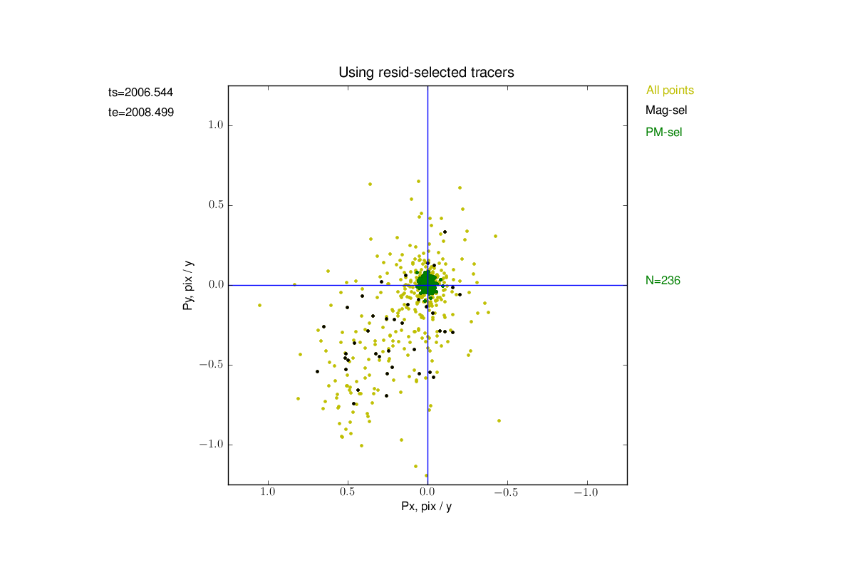
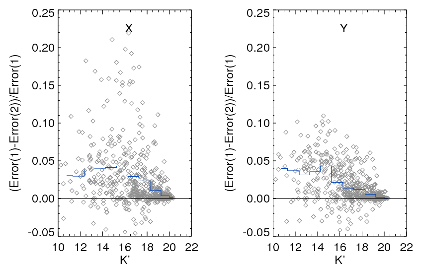
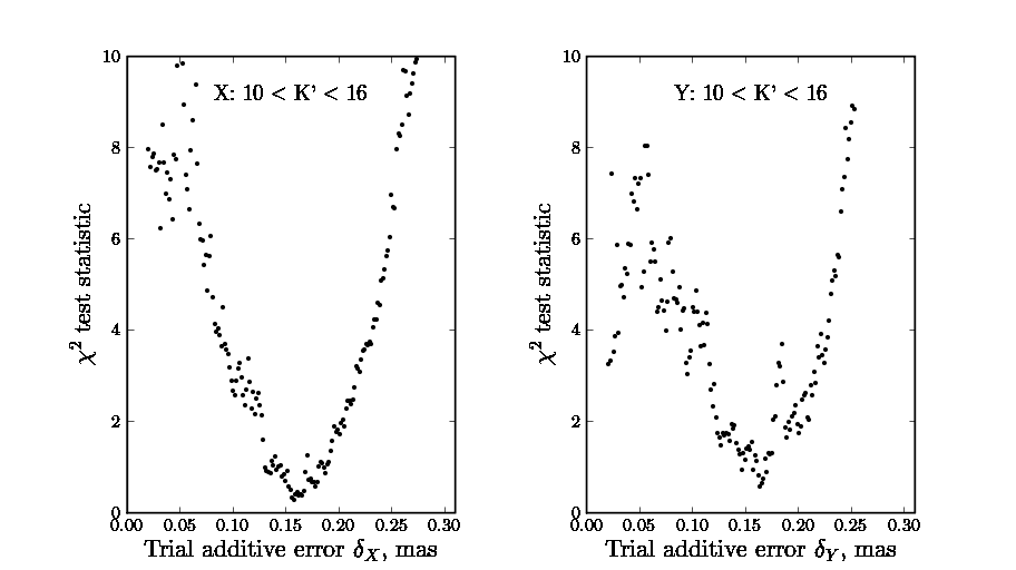
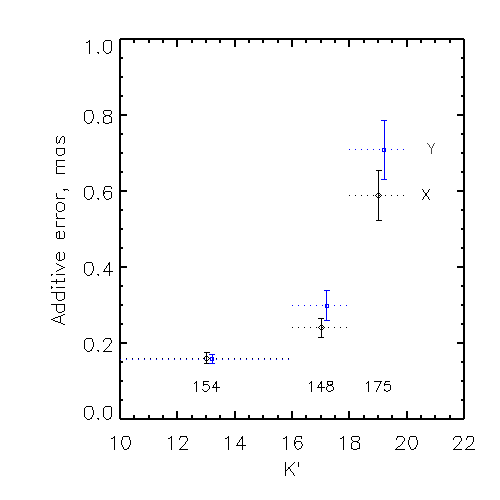
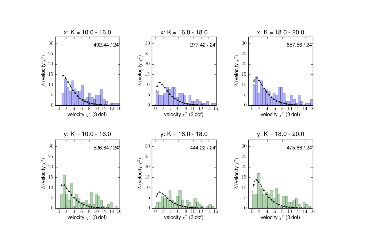
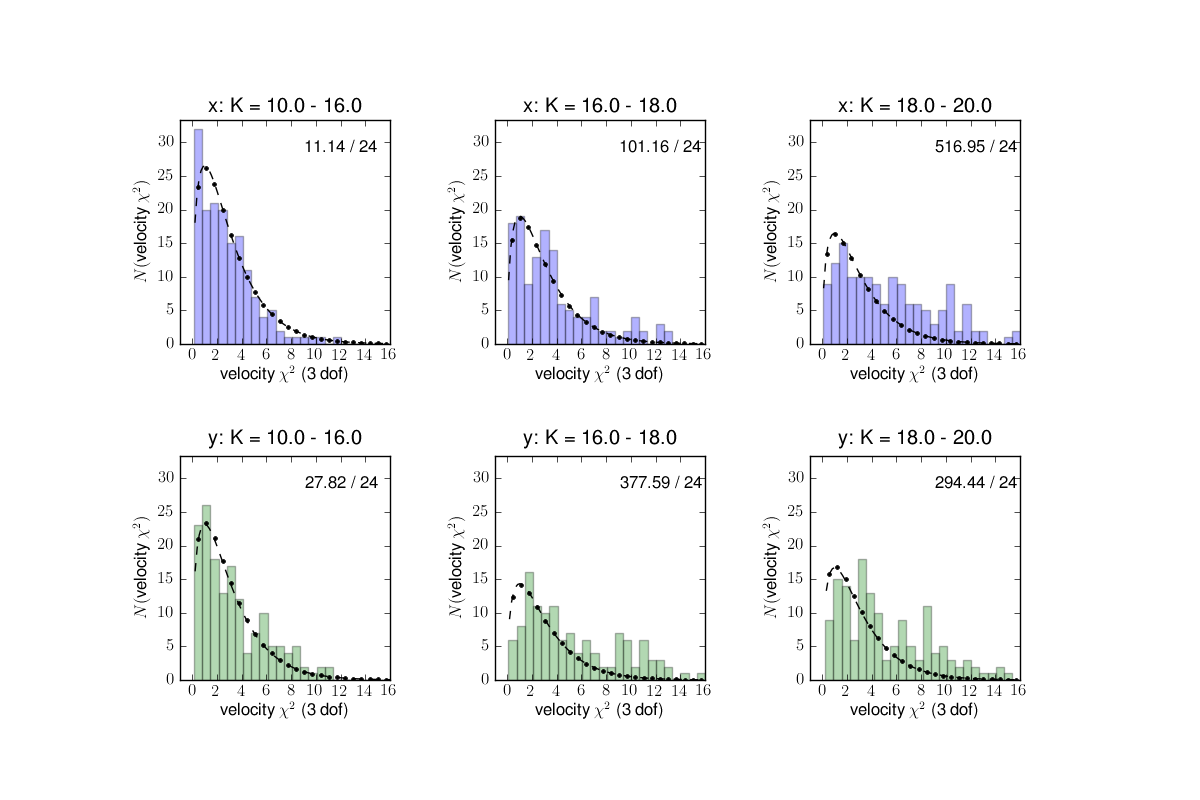
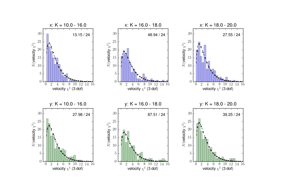
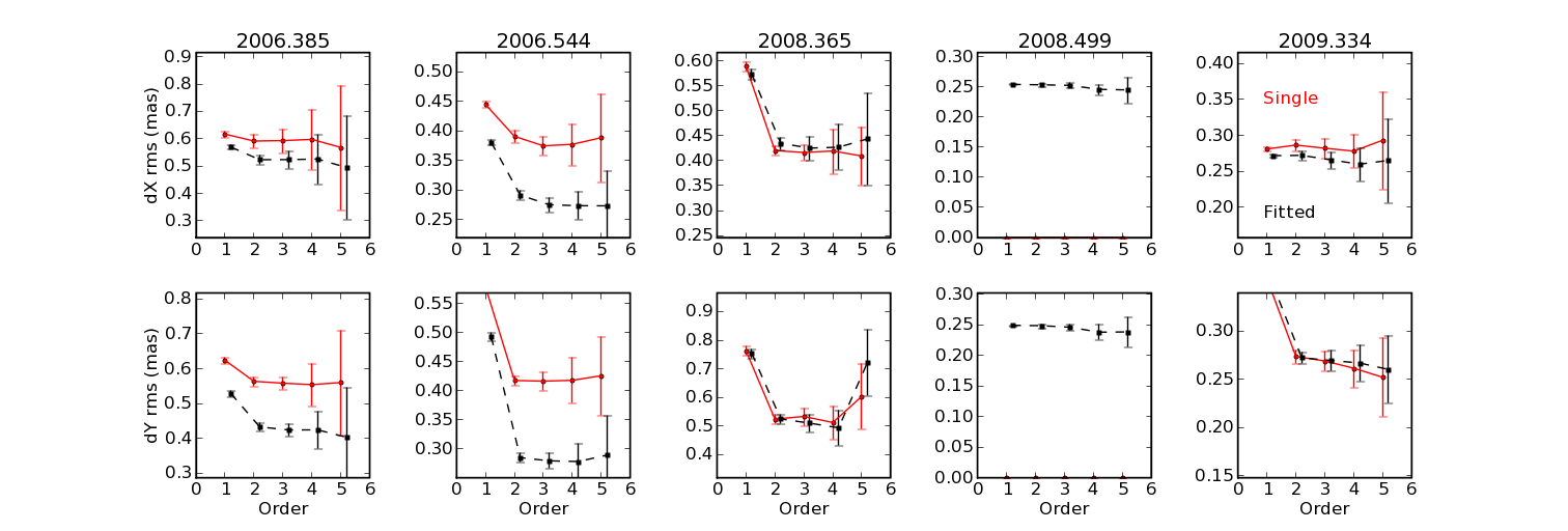
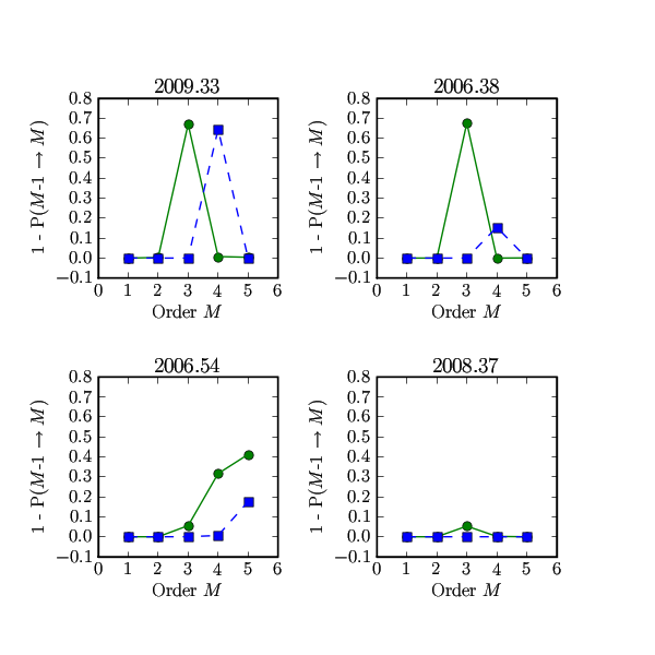
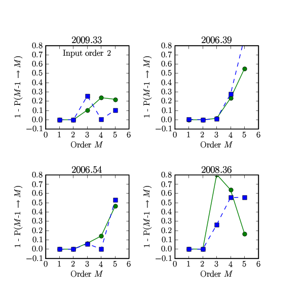
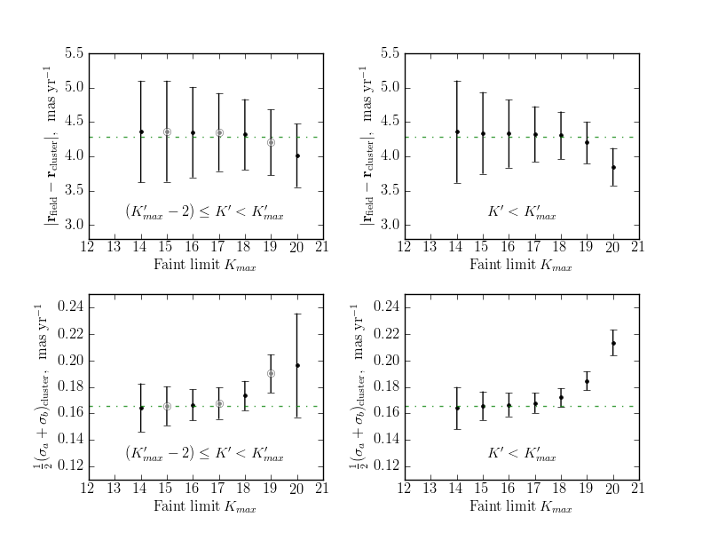
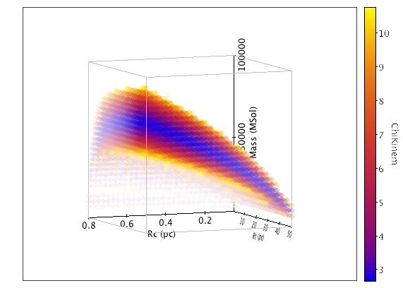
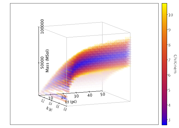
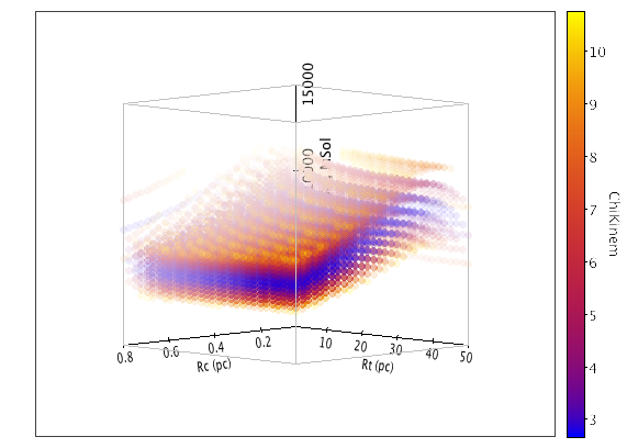
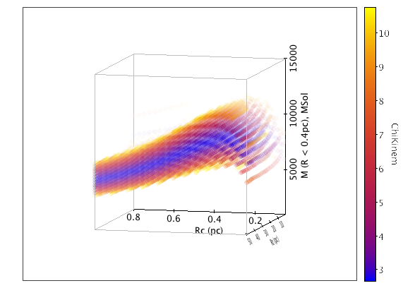
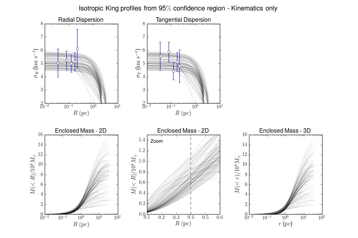
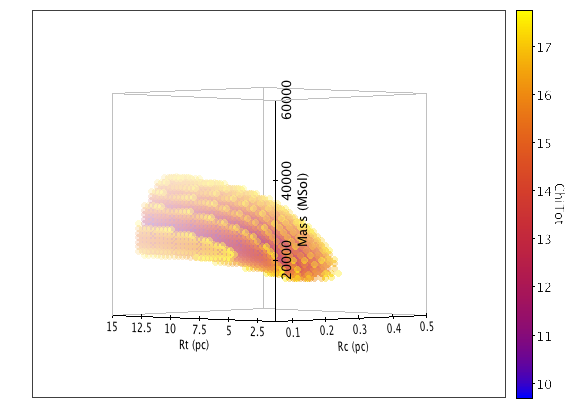
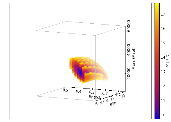
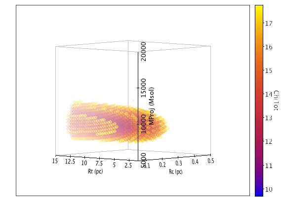
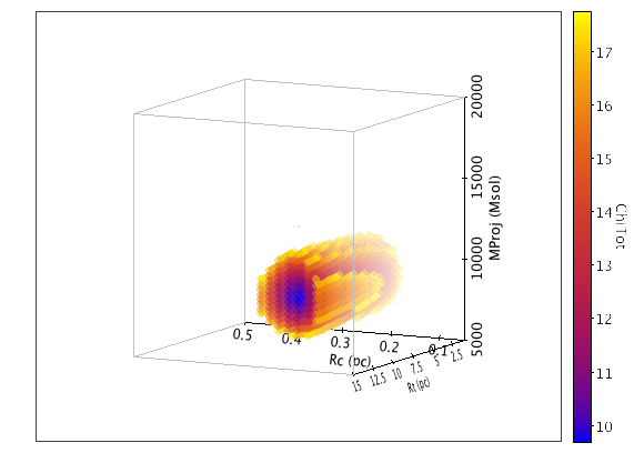
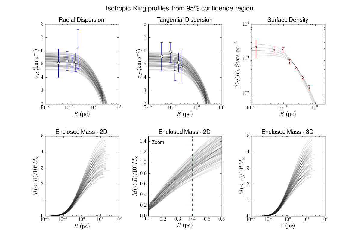
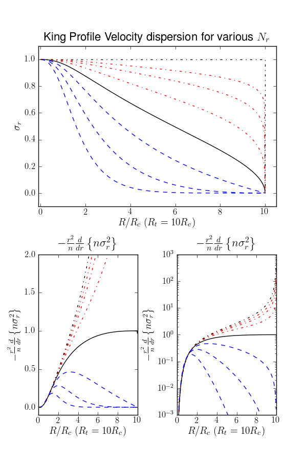
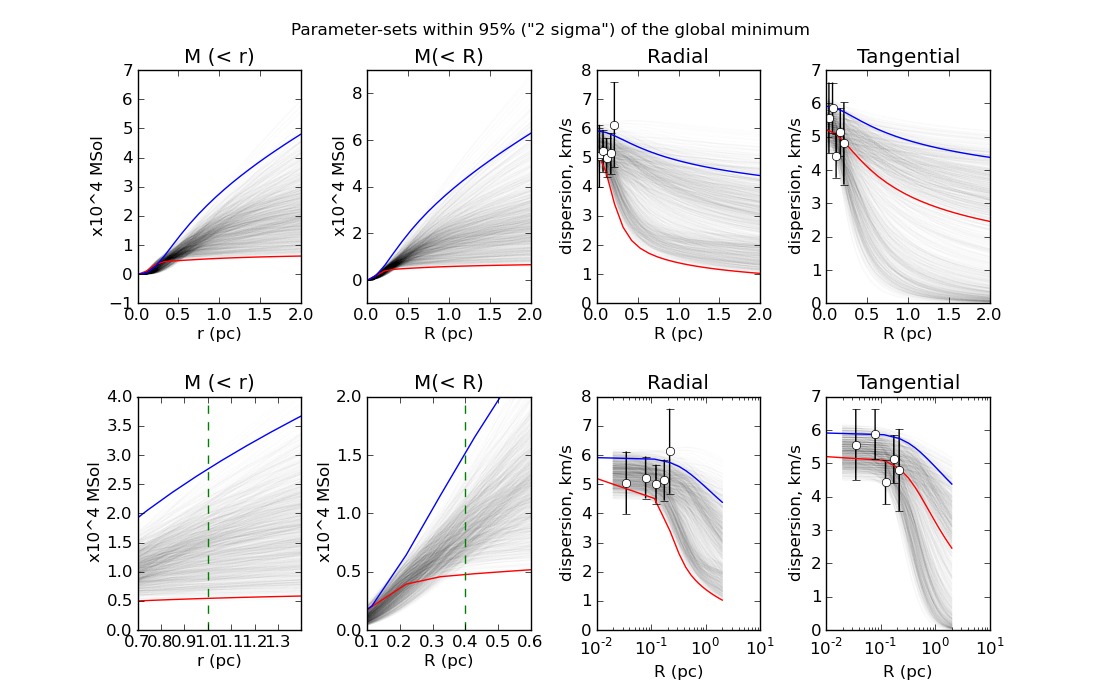
$\Delta\chi^{2}_{kinem}$	3.50	7.82	13.93
Confidence	68%	95%	99.7%
	”$1\sigma$”	”$2\sigma$”	”$3\sigma$”
$M(R<0.40~{}{\rm pc})$	0.40 - 1.10	0.36 - 1.19	0.32 - 1.30
($10^{4}~{}M_{\odot}$)
$M(r<1.0~{}{\rm pc})$	0.74 - 1.98	0.50 - 2.14	0.50 - 2.33
($10^{4}~{}M_{\odot}$)
$\rho_{0}$	0.06 - 30.92	0.05 - 30.92	0.05 - 31.40
($10^{5}M_{\odot}~{}{\rm pc^{-3}}$)
$R_{c}$	0.05 - 0.80	0.05 - 0.80	0.05 - 0.80
(pc)
$R_{t}$	1.00 - 50.00	1.00 - 50.00	1.00 - 50.00
(pc)
$M_{cluster}$	0.83 - 8.36	0.50 - 9.34	0.50 - 10.00
($10^{4}~{}M_{\odot}$)

Table 11: Significance regions for isotropic King modeling of the Arches cluster. Ranges of each parameter corresponding to the stated significance level are given, when $R_{c},R_{t},M_{cluster}$ are all allowed to vary. The quantity $\chi^{2}_{kinem}$ denotes the badness-of-fit when comparing model predictions to the Arches kinematic dataset only.

$\Delta\chi^{2}_{full}$	3.50	7.82	13.93
Confidence	68%	95%	99.7%
	”$1\sigma$”	”$2\sigma$”	”$3\sigma$”
$M(R<0.40~{}{\rm pc})$	0.70 - 1.10	0.62 - 1.20	0.56 - 1.30
($10^{4}~{}M_{\odot}$)
$M(r<1.0~{}{\rm pc})$	1.07 - 1.77	0.96 - 1.92	0.85 - 2.11
($10^{4}~{}M_{\odot}$)
$\rho_{0}$	0.89 - 2.37	0.62 - 3.47	0.44 - 3.91
($10^{5}M_{\odot}~{}{\rm pc^{-3}}$)
$R_{c}$	0.15 - 0.21	0.13 - 0.26	0.13 - 0.33
(pc)
$R_{t}$	3.00 - 30.00	2.00 - 30.00	2.00 - 30.00
(pc)
$M_{cluster}$	1.64 - 3.53	1.26 - 3.91	1.07 - 4.48
($10^{4}~{}M_{\odot}$)
$1000\times\Sigma_{N,0}/\rho_{0}$	0.00 - 0.01	0.00 - 0.06	0.00 - 0.12
(stars pc${}^{-2}/M_{\odot}~{}{\rm pc}^{-3}$)

Table 12: Significance regions for isotropic King modeling of the Arches cluster. Ranges of each parameter corresponding to the stated significance level are given, when $R_{c},R_{t},M_{cluster}$ are all allowed to vary. The quantity $\chi^{2}_{full}$ denotes the badness-of-fit when comparing model predictions to both the Arches kinematic dataset and the surface density dataset of Espinoza et al. (2009), over the mass range ($10\leq M\leq 120$) $M_{\odot}$.

References

- Allison et al. (2009) Allison, R. J., Goodwin, S. P., Parker, R. J., de Grijs, R., Portegies Zwart, S. F. & Kouwenhoven, M. B. N. 2009 ApJ, 700, 99
- Anderson & van der Marel (2010) Anderson, J., & van der Marel, R. P. 2010, ApJ, 710, 1032
- Babusiaux et al. (2010) Babusiaux, C., et al. 2010, A&A, 519, A77
- Bartko et al. (2010) Bartko, H., et al. 2010, ApJ, 708, 834
- Bastian et al. (2008) Bastian, N., Gieles, M., Goodwin, S. P., Trancho, G., Smith, L. J., Konstantopoulos, I. & Efremov, Y. 2008, MNRAS,389, 323
- Bastian et al. (2010) Bastian, N., Covey, K. R., & Meyer, M. R. 2010, ARA&A, 48, 339
- Benjamin et al. (2005) Benjamin, R. A., et al. 2005, ApJ, 630, L149
- Bevington & Robinson (2003) Bevington, P. R., & Robinson, D. K. 2003, Data reduction and error analysis for the physical sciences, 3rd ed., by Philip R. Bevington, and Keith D. Robinson. Boston, MA: McGraw-Hill, ISBN 0-07-247227-8, 2003.
- Bishop (2008) Bishop, C. M. 2006, Pattern Recognition and Machine Learning, 1st ed., by Christopher M. Bishop. New York, NY: Springer, ISBN -10: 0-387-31073-8
- Bonnell et al. (2004) Bonnell, I. A., Vine, S. G., & Bate, M. R. 2004, MNRAS, 349, 735
- Bonnell & Rice (2008) Bonnell, I. A., & Rice, W. K. M. 2008, Science, 321, 1060
- Bovy et al. (2009) Bovy, J., Hogg, D. W., & Roweis, S. T. 2009, arXiv:0905.2979
- Cabrera-Lavers et al. (2007) Cabrera-Lavers, A., Hammersley, P. L., González-Fernández, C., López-Corredoira, M., Garzón, F., & Mahoney, T. J. 2007, A&A, 465, 825
- Cotera et al. (1996) Cotera, A. S., Erickson, E. F., Colgan, S. W. J., Simpson, J. P., Allen, D. A., & Burton, M. G. 1996, ApJ, 461, 750
- Chatterjee et al. (2009) Chatterjee, S., Goswami, S., Umbreit, S., Glebbeek, E., Rasio, F. A., & Hurley, J. 2009, arXiv:0911.1483
- Clarkson et al. (2008) Clarkson, W., et al. 2008, ApJ, 684, 1110
- Crowther et al. (2010) Crowther, P. A., Schnurr, O., Hirschi, R., Yusof, N., Parker, R. J., Goodwin, S. P., & Kassim, H. A. 2010, MNRAS, 408, 731
- Dib (2007) Dib, S. 2007, Journal of Korean Astronomical Society, 40, 157
- Diolaiti et al. (2000) Diolaiti, E., Bendinelli, O., Bonaccini, D., Close, L., Currie, D., & Parmeggiani, G. 2000, A&AS, 147, 335
- Dwek et al. (1995) Dwek, E., et al. 1995, ApJ, 445, 716
- Elmegreen et al. (2008) Elmegreen, B. G., Klessen, R. S., & Wilson, C. D. 2008, ApJ, 681, 365
- Espinoza et al. (2009) Espinoza, P., Selman, F. J., & Melnick, J. 2009, A&A, 501, 563
- Figer et al. (1999) Figer, D. F., Kim, S. S., Morris, M., Serabyn, E., Rich, R. M., & McLean, I. S. 1999, ApJ, 525, 750
- Figer et al. (2002) Figer, D. F., et al. 2002, ApJ, 581, 258
- Figer (2005) Figer, D. F. 2005, Nature, 434, 192
- Fritz et al. (2010) Fritz, T., et al. 2010, MNRAS, 401, 1177
- Fruchter & Hook (2002) Fruchter, A. S., & Hook, R. N. 2002, PASP, 114, 144
- Ghez et al. (2005) Ghez, A. M., et al. 2005, ApJ, 635, 1087
- Ghez et al. (2008) Ghez, A. M., et al. 2008, ApJ, 689, 1044
- Gieles et al. (2010) Gieles, M., Sana, H., & Portegies Zwart, S. F. 2010, MNRAS, 402, 1750
- Gillessen et al. (2009) Gillessen, S., Eisenhauer, F., Trippe, S., Alexander, T., Genzel, R., Martins, F., & Ott, T. 2009, ApJ, 692, 1075
- Harayama et al. (2008) Harayama, Y., Eisenhauer, F., & Martins, F. 2008, ApJ, 675, 1319
- Harfst et al. (2010) Harfst, S., Portegies Zwart, S., & Stolte, A. 2010, MNRAS, 409, 628
- Howard et al. (2009) Howard, C. D., et al. 2009, ApJ, 702, L153
- Jones & Walker (1988) Jones, B. F., & Walker, M. F. 1988, AJ, 95, 1755
- Kim et al. (1999) Kim, S. S., Morris, M., & Lee, H. M. 1999, ApJ, 525, 228
- Kim et al. (2000) Kim, S. S., Figer, D. F., Lee, H. M., & Morris, M. 2000, ApJ, 545, 301
- Kim & Morris (2003) Kim, S. S., & Morris, M. 2003, ApJ, 597, 312
- Kim et al. (2006) Kim, S. S., Figer, D. F., Kudritzki, R. P., & Najarro, F. 2006, ApJ, 653, L113
- King (1962) King, I. 1962, AJ, 67, 471
- King (2008) King, I. R. 2008, IAU Symposium, 246, 131
- Klessen et al. (2007) Klessen, R. S., Spaans, M., & Jappsen, A.-K. 2007, MNRAS, 374, L29
- Kozhurina-Platais et al. (1995) Kozhurina-Platais, V., Girard, T. M., Platais, I., van Altena, W. F., Ianna, P. A., & Cannon, R. D. 1995, AJ, 109, 672
- Kroupa (2002) Kroupa, P. 2002, Science, 295, 82
- Krumholz & McKee (2008) Krumholz, M. R., & McKee, C. F. 2008, Nature, 451, 1082
- Kuijken & Rich (2002) Kuijken, K., & Rich, R. M. 2002, AJ, 124, 2054
- Lampton et al. (1976) Lampton, M., Margon, B., & Bowyer, S. 1976, ApJ, 208, 177
- Lang (2004) Lang, C. C. 2004, The Formation and Evolution of Massive Young Star Clusters, 322, 179
- Launhardt et al. (2002) Launhardt, R., Zylka, R., & Mezger, P. G. 2002, A&A, 384, 112
- Lecureur et al. (2007) Lecureur, A., Hill, V., Zoccali, M., Barbuy, B., Gómez, A., Minniti, D., Ortolani, S., & Renzini, A. 2007, A&A, 465, 799
- Lejeune & Schaerer (2001) Lejeune, T., & Schaerer, D. 2001, A&A, 366, 538
- Leonard & Merritt (1989) Leonard, P. J. T., & Merritt, D. 1989, ApJ, 339, 195
- Leonard et al. (1992) Leonard, P. J. T., Richer, H. B., & Fahlman, G. G. 1992, AJ, 104, 2104
- Lu et al. (2009) Lu, J. R., Ghez, A. M., Hornstein, S. D., Morris, M. R., Becklin, E. E., & Matthews, K. 2009, ApJ, 690, 1463
- Martins et al. (2008) Martins, F., Hillier, D. J., Paumard, T., Eisenhauer, F., Ott, T., & Genzel, R. 2008, A&A, 478, 219
- McCrady et al. (2011) McCrady, N., Lu, J., Clarkson, W., Ghez, A., Morris, M. R., Stolte, A., & Yelda, S. 2011, Astronomical Society of the Pacific Conference Series, 439, 121
- McKee & Ostriker (2007) McKee, C. F., & Ostriker, E. C. 2007, ARA&A, 45, 565
- McWilliam & Rich (1994) McWilliam, A., & Rich, R. M. 1994, ApJS, 91, 749
- McWilliam & Zoccali (2010) McWilliam, A., & Zoccali, M. 2010, ApJ, 724, 1491
- Miller & Scalo (1979) Miller, G. E., & Scalo, J. M. 1979, ApJS, 41, 513
- Morris & Yusef-Zadeh (1989) Morris, M., & Yusef-Zadeh, F. 1989, ApJ, 343, 703
- Morris (1993) Morris, M. 1993, ApJ, 408, 496
- Morris & Serabyn (1996) Morris, M., & Serabyn, E. 1996, ARA&A, 34, 645
- Nagata et al. (1995) Nagata, T., Woodward, C. E., Shure, M. & Kobayashi, N. 1995, AJ, 109, 167
- Najarro et al. (2004) Najarro, F., Figer, D. F., Hillier, D. J., & Kudritzki, R. P. 2004, ApJ, 611, L105
- Platais et al. (2003) Platais, I., Kozhurina-Platais, V., Mathieu, R. D., Girard, T. M., & van Altena, W. F. 2003, AJ, 126, 2922
- Portegies Zwart et al. (2002b) Portegies Zwart, S. F., Makino, J., McMillan, S. L. W., & Hut, P. 2002, ApJ, 565, 265
- Portegies Zwart et al. (2007) Portegies Zwart, S., Gaburov, E., Chen, H.-C., Guerkan, M. A. 2007, MNRAS, 378, L29
- Portegies Zwart et al. (2010) Portegies Zwart, S. F., McMillan, S. L. W., & Gieles, M. 2010, ARA&A, 48, 431
- Press (2002) Press, W. H. 2002, Numerical recipes in C++ : the art of scientific computing by William H. Press. xxviii, 1,002 p. : ill. ; 26 cm. Includes bibliographical references and index. ISBN : 0521750334,
- Robin et al. (2009) Robin, A. C., Marshall, D. J., Reylé, C., & Schultheis, M. 2009, SF2A-2009: Proceedings of the Annual meeting of the French Society of Astronomy and Astrophysics, 221
- Salpeter (1955) Salpeter, E. E. 1955, ApJ, 121, 161
- Sanders (1971) Sanders, W. L. 1971, A&A, 14, 226
- Schödel et al. (2009) Schödel, R., Merritt, D., & Eckart, A. 2009, A&A, 502, 91
- Serabyn et al. (1998) Serabyn, E., Shupe, D., & Figer, D. F. 1998, Nature, 394, 448
- Shen et al. (2010) Shen, J., Rich, R. M., Kormendy, J., et al. 2010, ApJ, 720, L72
- Soto et al. (2007) Soto, M., Rich, R. M., & Kuijken, K. 2007, ApJ, 665, L31
- Stolte et al. (2002) Stolte, A., Grebel, E. K., Brandner, W., & Figer, D. F. 2002, A&A, 394, 459
- Stolte et al. (2005) Stolte, A., Brandner, W., Grebel, E. K., Lenzen, R., & Lagrange, A.-M. 2005, ApJ, 628, L113
- Stolte et al. (2008) Stolte, A., Ghez, A. M., Morris, M., Lu, J. R., Brandner, W., & Matthews, K. 2008, ApJ, 675, 1278
- Stolte et al. (2010) Stolte, A., et al. 2010, ApJ, 718, 810
- van Dam et al. (2006) van Dam, M. A., et al. 2006, PASP, 118, 310
- Wizinowich et al. (2006) Wizinowich, P. L., et al. 2006, PASP, 118, 297
- Yelda et al. (2010) Yelda, S., Lu, J. R., Ghez, A. M., Clarkson, W., Anderson, J., Do, T., & Matthews, K. 2010, ApJ, 725, 331 (Y10)
- Yusef-Zadeh et al. (1984) Yusef-Zadeh, F., Morris, M., & Chance, D. 1984, Nature, 310, 557
- Yusef-Zadeh et al. (2002) Yusef-Zadeh, F., Law, C., Wardle, M., Wang, Q. D., Fruscione, A., Lang, C. C., & Cotera, A. 2002, ApJ, 570, 665
- Zhao et al. (1994) Zhao, H., Spergel, D. N., & Rich, R. M. 1994, AJ, 108, 2154