Observational Constraints on finite scale factor singularities
Abstract
We discuss the combined constraints on a Finite Scale Factor Singularity (FSF) universe evolution scenario, which come from the shift parameter , baryon acoustic oscillations (BAO) , and from the type Ia supernovae. We show that observations allow existence of such singularities in the years in future (at CL) which is much farther than a Sudden Future Singularity (SFS), and that at the present moment of the cosmic evolution, one cannot differentiate between cosmological scenario which allow finite scale factor singularities and the standard CDM dark energy models. We also show that there is an allowed value of within CL, which corresponds to a dust-filled Einstein-de-Sitter universe limit of the early time evolution and so it is pasted ito a standard early-time scenario.
pacs:
98.80.Es; 98.80.Cq; 04.20.DwI Introduction
Finite scale factor singularities (FSF) are one of types of new and exotic singularities which were found first in Ref. BGT . The inspiration to search these new types of singularities was due to the observations of high-redshift type Ia supernovae (SNIa) which provided strong evidence that the expansion of the universe is accelerating due to an unknown form of dark energysupernovaeold phenomenologically behaving as the cosmological constant. Further observational data supernovaenew made cosmologists think of more accelerating universe filled with phantom phantom which violated all energy conditions: the null (), weak ( and ), strong ( and ), and dominant energy (, ) ( is the speed of light, is the mass density in and is the pressure). Phantom-driven dark energy leads to a big-rip singularity (BR or type I according to nojiri ) in which the infinite values of the energy density and pressure (, ) are accompanied by the infinite value of the scale factor () caldwellPRL .
The list of new types of singularities contains: a big-rip (BR), a sudden future singularity (SFS) barrow04 , which can appear in inhomogeneous and anisotropic models too barrow042 ; sfs1 , a generalized sudden future singularity (GSFS), a finite scale factor singularity (FSF) aps , a big-separation singularity (BS). They are characterized by violation of all or some of the energy conditions which results in a blow-up of all or some of the physical quantities: the scale factor, the energy density and the pressure. The finite scale factor singularity, which is the subject of this paper, is a weak singularity according to Tipler’s definition, but strong according to Królak’s definition lazkoz . Apart from mentioned above there are also -singularities wsin , which are not physical singularities, but are singularities of a barotropic index which are present in different cosmological models of gravity star1980 , in scalar field models Setare , and in brane cosmologies Sahni .
For a finite scale factor singularity (FSF) and diverge, while the scale factor remains constant. This means that it is similar to a big-bang singularity with only one exception - the scale factor is a constant const instead of zero . Besides, FSF singularities are stronger than a sudden future singularities (SFS) [10], so they placed themselves in between the big-bang (which is strong and geodesically incomplete) and the SFS. It has been shown that SFS appear in physical theories such as gravity, scalar field cosmologies, brane cosmologies yuri and, in particular, they plague loop quantum cosmology LQC . It seems then that after an appropriate choice of the scalar field, function or brane, FSF will be easily deduced to appear in such physical theories as well.
The paper is organized as follows. In section II we present FSF scenario. In section III we derive the expressions for the observables: baryon acoustic oscillations, distance to the last scattering surface, type Ia supernovae, used to test an FSF scenario. In section IV we give the results and discussion.
II Finite Scale Factor Singularity scenario construction
In order to obtain an FSF singularity one should consider the simple framework of an Einstein-Friedmann cosmology governed by the standard field equations
| (II.1) | |||||
| (II.2) |
where the energy-momentum conservation law
| (II.3) |
is trivially fulfilled due to the Bianchi identity. Here is the scale factor, the dot means the derivative with respect to time , is the gravitational constant, and the curvature index . During further considerations we set and .
Similarly like in the case of SFS, which were tested against the observations in DHD ; GHDD ; DDGH , one is able to obtain an FSF singularity by taking the scale factor in the form
| (II.4) |
with the appropriate choice of the constants . In contrast to an SFS in order to have accelerated expansion of the universe has to be positive (). For we have an SFS, which plagues the loop quantum cosmology LQC . In order to have an FSF singularity instead of SFS, has to lie in the range .
As can be seen from (II.1)-(II.4), for an FSF diverges and we have: for , , , and , where , are constants and .
In a model, expressed in terms of the scale factor (II.4), the evolution begins with the standard big-bang singularity at for , and finishes at a finite scale factor singularity for where is a constant. In terms of the rescaled time we have .
The standard Friedmann limit (i.e. models without a singularity) of
(II.4) is achieved when ; hence is called
the “non-standardicity” parameter. Additionally,
notwithstanding Ref. barrow04 and in agreement with the field
equations (II.1)-(II.2), can be
both positive and negative leading to an acceleration or a
deceleration of the universe,
respectively.
It is important to our discussion that the asymptotic behaviour of the scale factor (II.4) close to the big-bang singularity at is given by a simple power-law , simulating the behaviour of flat barotropic fluid models with .
The FSF singularity scenario consists of two dominating components such as a nonrelativistic matter, and the fluid which is driving the singularity. We consider the case of the noninteracting components from which both of them obey independently their continuity equations as II.3.
The evolution of both ingredients is independent. Nonrelativistic matter scales as
| (II.5) |
and the evolution of the other fluid, which we name here , can be determined by taking the difference between whole energy density, , evolution from Friedmann eq. II.1 and the :
| (II.6) |
this ingredient, , of the content of the Universe is responsible for the singularity in the energy density for .
II.1 Classical stability of FSFS with respect to small perturbations
In Ref. JBSZWL the study of classical stability of sudden singularities and “Big Rip” singularities with respect to small inhomogeneous scalar, vector and tensor perturbations was given. The analysis was made in the framework of gauge-invariant formalism introduced by Mukhanov MUK2 . Characterization of sudden singularities in terms of the series expansion of the scale factor on the approach to a singularity was given, and it was shown that once the density diverges near to a singularity it is unstable under small scalar perturbations. On the other hand, sudden singularities are stable to inhomogeneous vector and (tensor) gravitational-wave perturbations. Taking the Friedmann equations (II.1)-(II.2) with , and the scale factor in terms of the series expansion on the approach to a singularity:
| (II.7) |
| (II.8) |
| (II.9) |
were the , are real constants, with , , in the limit the approximation for the density and pressure was derived JBSZWL :
| (II.10) |
| (II.11) |
The density diverges if and only if , and the pressure diverges, if . Substituting (II.7-II.11) into the gauge-invariant scalar perturbations equation MUK2 :
| (II.12) |
for plane wave perturbations with wave number , where , and further neglecting higher-order terms, and taking the case of we have JBSZWL :
| (II.13) |
where and dots indicate differentiation with respect to . By transformation of the variables, one can express this equation as the Bessel equation, and then obtain its solution to be JBSZWL :
| (II.14) |
where , are constants. For FSFS with , diverges as . Such a result is valid for all wavelengths, and for all values of .
III Observational constraints
We consider three observational constraints, such as luminosity distance moduli to type Ia supernovae, baryon acoustic oscillations, and the shift parameter which is scaled distance to the last scattering surface of the cosmic microwave background. We make use of Markov Chain Monte Carlo technique within the framework of Bayesian statistics to obtain posterior probability distribution as a function of the parameters: , , , , where is the present age of the universe. We employ Metropolis-Hastings algorithm with uniform priors: , , , . The results are marginalised over taken from HST Key Project.
III.1 Supernovae
We proceed within the framework of Friedmann cosmology, and consider an observer located at at coordinate time . The observer receives a light ray emitted at at coordinate time . We then have a standard null geodesic equation
| (III.1) |
with the scale factor given by (II.4). Using (II.4) again, the redshift is given by
| (III.2) |
where and .
The luminosity distance to supernova is given by
| (III.3) |
and the distance modulus is
| (III.4) |
The for the SNIa data is
| (III.5) |
where is the quoted observational error on the Union2 SNIa and is the SNIa intrinsic scatter. Following Amanullah we take .
III.2 Shift parameter
The standard formula for the CMB shift parameter is given by bond97 ; Nesseris:2006er :
| (III.6) |
where is the temperature perturbation CMB spectrum multipole of the first acoustic peak in the model under consideration and corresponds to a reference flat standard Cold Dark Matter (CDM) model. The multipole number is related to an angular scale of the sound horizon at decoupling by PRD41 ; singh03
| (III.7) |
where
| (III.8) |
with being the sound velocity and the angular diameter distance reads as
| (III.9) |
where is the velocity of light and for .
Following Nesseris:2006er we can write, using (III.6) and (III.7) as follows
| (III.10) |
which, by assuming that at decoupling the amount of radiation was the same in both the flat reference standard CDM model and in our FSF model (which we assume to be just the same as a standard matter-radiation model of the early universe, since FSF models do not change the evolution there) we have that
| (III.11) |
On the other hand, for a reference standard CDM model
| (III.12) | |||||
while for our FSF model the angular diameter distance is given by
| (III.13) |
with given by taken at decoupling. Using the above, we may write that for our FSF models the shift parameter is
| (III.14) |
where we have assumed that the function is approximately unity Nesseris:2006er .
Finally, the rescaled shift parameter is
| (III.15) | |||||
where . The WMAP data gives 7y , thus for the shift parameter is the following
| (III.16) |
III.3 Baryon acoustic oscillations
In Ref. eisenstein it was suggested that instead of taking the position of an acoustic peak one should measure the large-scale correlation function at Mpc separation using the sample of 46748 luminous red galaxies (LRG) selected from the SDSS (Sloan Digital Sky Survey) sample. The appropriate quantity to be measured is known as the parameter and reads as
| (III.17) |
According to Ref. eisenstein should have the value
| (III.18) |
where is the spectral index (now taken about ).
We have for BAO
| (III.19) |
Using (II.4) and (III.2) we get the form of for an FSF as follows
| (III.20) |
|
||
|
|
|
|
|
|
IV Results and Conclusions
Overall that has been used is
| (IV.1) |
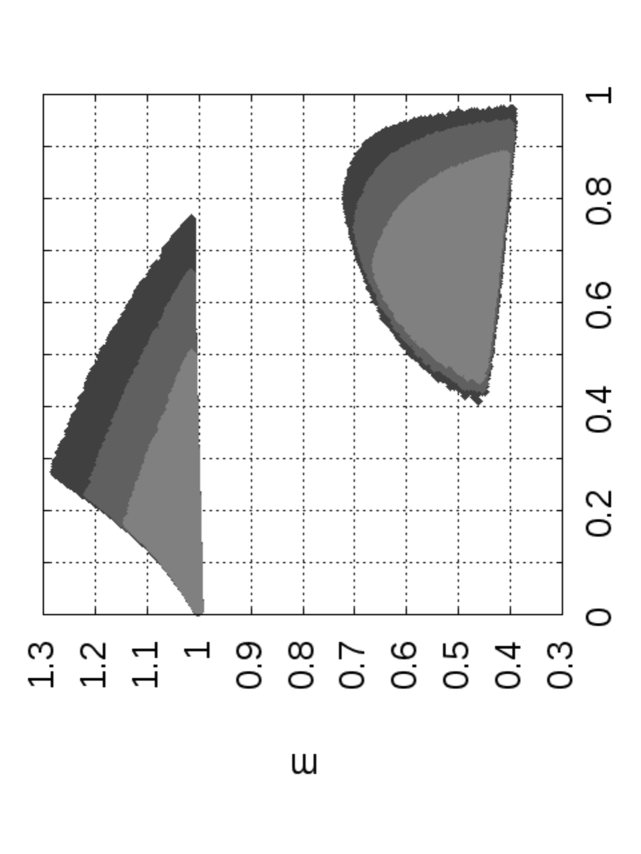
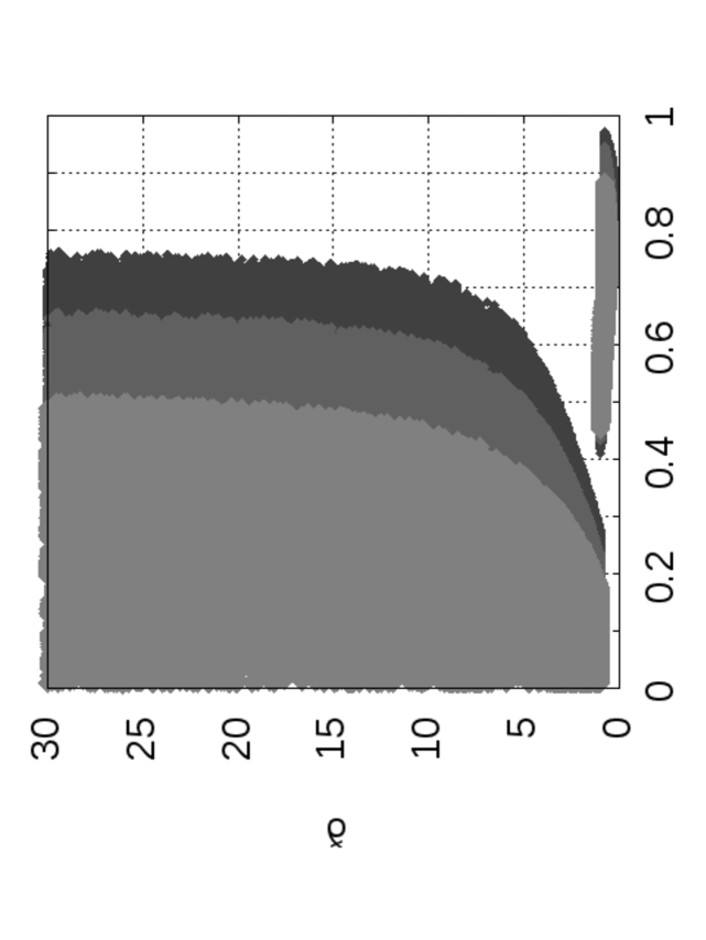
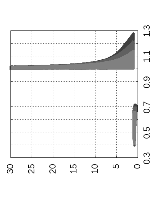
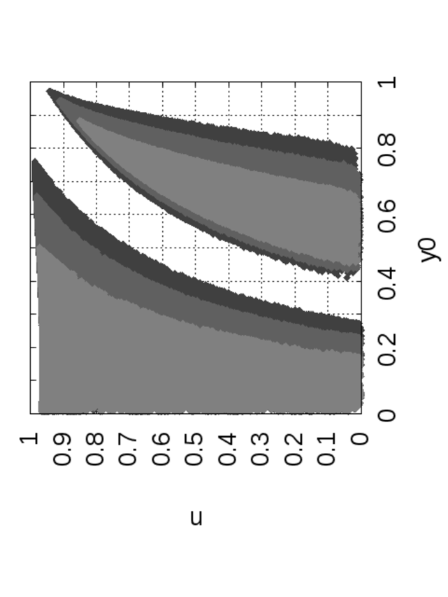
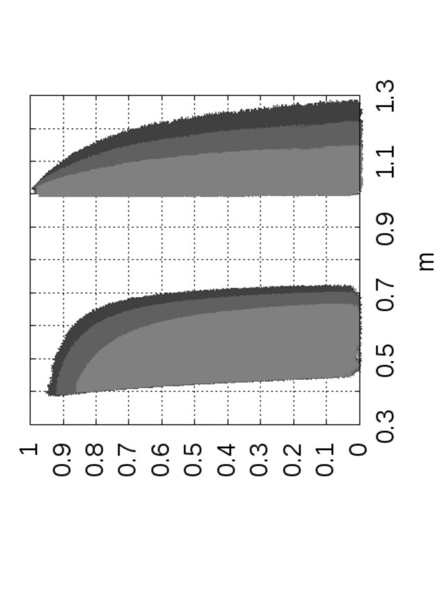
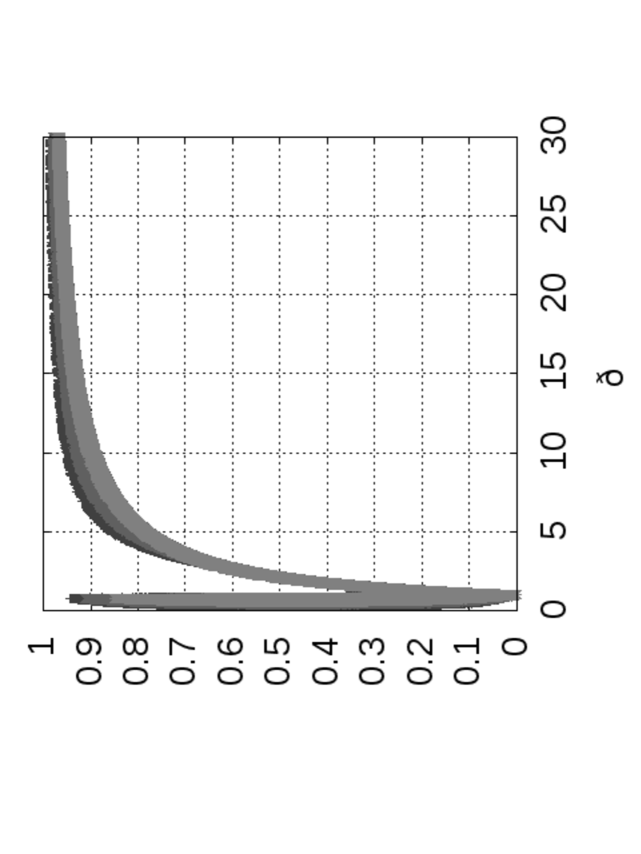
In Fig. 1 we present contour plots showing the joint marginal posterior distribution for each pair of FSF model parameters. Each sub-panel shows three contours, denoting roughly 68%, 95% and 99% (from light gray to dark grey respectively) credible regions.
In Fig. 1 we see that there are two disjoined regions in the parameter space for which FSF singularities are allowed in the universe. is always positive which is not surprising since only for positive there can be an accelerated expansion in the investigated model. Characteristic feature of the picture is that there are two qualitatively different regions divided by the value of the parameter . There are two branches, the first for , and the second for . In the following tables we present ranges of the values of the parameters for three confidence levels. For the case when :
| CL | CL | CL |
|---|---|---|
Below the case of :
| CL | CL | CL |
|---|---|---|
For the case of the branch the maximum value at parameter is , which means that such a singularity can happen later than for the second branch . While approaches , grows stronger and as the value of more grows, becomes better constrained.
What seems to be important is that there is an allowed value of within CL, which could correspond to the dust filled Einstein-de-Sitter universe in a close to big-bang limiting case. What is also interesting for this branch is that while the allowed values of the nonstandarcity parameter are small, i.e. , the parameter approaches unity which means that the singularity may happen in the nearest future for this case. For CL, corresponds to years to the time of the singularity. For CL, corresponds to the present time at years before the time of the singularity.
In conclusion, we have shown that for a finite scale factor singularity there is an allowed value of within CL,
which corresponds to the dust-filled Einstein-de-Sitter universe for the close to big-bang limiting case.
The finite scale factor singularity may
happen within years in future for CL and its prediction at the present moment of cosmic
evolution cannot be distinguished, with current observational data,
from the prediction given by the standard quintessence scenario of
future evolution in the Concordance Model chevallier00 ; linder02 ; linder05 ; koivisto05 ; caldwell07 ; zhang07 ; amendola07 ; diporto07 ; hu07b ; linder09 .
V Acknowledgements
I warmly thank A. Balcerzak, M.P. Da̧browski, M.A. Hendry, and Yu.V. Shtanov for comments and discussions.
I acknowledge the support of the National Science Center grant No N N202 3269 40 (years 2011-2013).
Part of the simulations reported in this work were performed using the HPC cluster HAL9000 of the Computing Centre of the Faculty of Mathematics and Physics at the University of Szczecin.
References
- (1) J.D. Barrow, G.J. Galloway and F.J. Tipler, Mon. Not. Roy. Astr. Soc., 223, 835 (1986);
- (2) S. Nojiri, S.D. Odintsov and S. Tsujikawa, Phys. Rev. D 71,063004 (2005).
- (3) S. Perlmutter et al., Astroph. J. 517, (1999) 565; A. G. Riess et al., Astron. J. 116, 1009 (1998); A.G. Riess et al., Astroph. J. 560, 49 (2001).
- (4) J.L. Tonry et al., Astroph. J. 594, 1 (2003); M. Tegmark et al., Phys. Rev. D69, 103501 (2004); R.A. Knop et al., Astrophys. J. 598, 102 (2003).
- (5) R.R. Caldwell, Phys. Lett. B 545, 23 (2002); M.P. Da̧browski, T. Stachowiak and M. Szydłowski, Phys. Rev. D 68, 103519 (2003); P.H. Frampton, Phys. Lett. B 562 (2003), 139; H. Štefančić, Phys. Lett. B586, 5 (2004); S. Nojiri and S.D. Odintsov, Phys. Lett. B595, 1 (2004).
- (6) R.R. Caldwell, M. Kamionkowski, and N.N. Weinberg, Phys. Rev. Lett. 91, 071301 (2003).
- (7) J.D. Barrow, Class. Quantum Grav. 21, L79 (2004).
- (8) J.D. Barrow and Ch. Tsagas, Class. Quantum Grav. 22, 1563 (2005).
- (9) J. D. Barrow and S. Z. W. Lip, Phys. Rev. D80, 043518 (2009).
- (10) V.F. Mukhanov, Physical Foundations of Cosmology, Cambridge University Press (2005), pp. 289-310.
- (11) V.F. Mukhanov, H.A. Feldman and R.H. Brandenberger, Phys. Rep., 215, 203 (1992)
- (12) M.P. Da̧browski, Phys. Rev. D71, 103505 (2005).
- (13) M.P. Da̧browski and T. Denkiewicz, AIP Conference Proceedings 1241, 561 (2010).
- (14) L. Fernandez-Jambrina and R. Lazkoz, Phys. Rev. D70, 121503(R) (2004); L. Fernandez-Jambrina and R. Lazkoz, Phys. Rev. D74, 064030 (2006).
- (15) M.P. Da̧browski and T. Denkiewicz, Phys. Rev. D79, 063521 (2009).
- (16) A. A. Starobinsky, Phys. Lett. 91B, 99 (1980).
- (17) M. R. Setare and E. N. Saridakis, Phys. Lett. B671, 331 (2009).
- (18) V. Sahni and Yu. Shtanov, Phys. Rev. D 71, 084018 (2005).
- (19) V. Sahni and Yu. Shtanov, Phys. Rev. D 71, 084018 (2005).
- (20) T. Cailleteau, A. Cardoso, K. Vandersloot, D. Wands Phys. Rev. Lett. 101, 251302 (2008); P. Singh, Class. Quantum Grav. 26, 125005 (2009).
- (21) M. P. Dabrowski, T. Denkiewicz, M. A. Hendry, Phys. Rev. D75, 123524 (2007).
- (22) H. Ghodsi, M. A. Hendry, M. P. Dabrowski, T. Denkiewicz, MNRAS, 414: 1517–1525 (2011).
- (23) T. Denkiewicz, M. P. Dabrowski, H. Ghodsi, M. A. Hendry, Phys. Rev. D85, 083527 (2012).
- (24) Amanullah et al. (The Supernova Cosmology Project), Astroph. J. 716, 712 (2010) [arXiv: 1004.1711].
- (25) J.R. Bond, G. Efstathiou, and M. Tegmark, [astro-ph/9702100].
- (26) S. Nesseris and L. Perivolaropoulos, JCAP 0701 (2007) 018 [arXiv:astro-ph/0610092].
- (27) J. Stelmach, R. Byrka, and M. P. Da̧browski, Phys. Rev. D41, 2434 (1990).
- (28) R.G. Vishwakarma and P. Singh, Class. Quantum Grav. 20, 2033 (2003).
- (29) N. Jarosik et al., The Astroph. J. Supplement Series, 192, 2 (2011).
- (30) D.J. Eisenstein, et al., ApJ, 633, 560 (2005) [astro-ph/0501171].
- (31) M. Chevallier and D. Polarski, Int. J. Mod. Phys. D10, 213 (2001).
- (32) E. V. Linder, Phys. Rev. Lett. 90, 091301 (2003).
- (33) E. V. Linder, Phys. Rev. D72, 043529 (2005).
- (34) T. Koivisto and D. F. Mota, Phys. Rev. D73, 083502 (2006).
- (35) R. Caldwell, A. Cooray and A. Melchiorri, Phys. Rev. D76, 023507 (2007).
- (36) P. Zhang, M. Liguori, R. Bean and S. Dodelson, Phys. Rev. Lett. 99, 141302 (2007).
- (37) L. Amendola, M. Kunz and D. Sapone, JCAP 0804, 013 (2008).
- (38) C. Di Porto and L. Amendola, Phys. Rev. D77, 083508 (2008).
- (39) W. Hu and I. Sawicki, Phys. Rev. D76, 104043 (2007).
- (40) E. V. Linder, Phys. Rev. D79, 063519 (2009).