Dynamical fluctuations close to Jamming versus Vibrational Modes : a pedagogical discussion illustrated on hard spheres simulations, colloidal and granular experiments

Abstract

Studying the jamming transition of granular and colloidal systems, has lead to a proliferation of theoretical and numerical results formulated in the language of the eigenspectrum of the dynamical matrix for these disordered system. Only recently however, these modes have been accessed experimentally in colloidal and granular media, computing the eigenmodes of the covariance matrix of the particle positions. At the same time new conceptual and methodological questions have appeared, regarding the interpretation of these results. In the present paper, we first give an overview of the theoretical framework which is appropriate to discuss the interpretation of the eigenmodes and eigenvalues of the correlation matrix in terms of the vibrational properties of these systems. We then illustrate several aspects of the statistical and data analysis techniques which are necessary to extract reliable results from experimental data. Concentrating on the case of hard sphere simulations, colloidal and granular experiments, we discuss how to test the existence of a metastable state, the statistical independence of the sampling, the effect of the experimental resolution, and the harmonic hypothesis underlying the approach, highlighting both its promises and limitations.

I Introduction

Amorphous systems such as structural glasses, colloids, emulsions or granular matter still lack a satisfying description. This is particularly apparent when one considers the low temperature properties of glasses Phillips (1978); Nakayama (2002) or the sometime intriguing rheological properties of athermal amorphous systems, such as foamsKatgert and van Hecke (2010); Tighe (2011) or granular matter van Hecke (2010); Dijksman et al. (2011). Of particular importance is the understanding of what guarantees the mechanical stability of such systems Alexander (1998); Wyart (2005) . The informations about the rigidity of a solid against collective particle motions are contained in the density of the vibrational modes $D(\omega)$: a system is stable – at least linearly – if there are no unstable modes. In a continuous isotropic elastic medium, the invariance by translation implies that the vibrational modes are plane waves and the density of vibrational modes $D(\omega)$ follows the Debye law $D(\omega)\sim\omega^{d-1}$Ashcroft and Mermin (1976), where $d$ is the space dimension. By contrast, disordered solids exhibit common low-frequency vibrational properties that are completely unlike those of crystals. Disordered atomic or molecular solids generically exhibit a “boson peak”, where many more modes appear than expected for sound Chumakov et al. (2004); Wyart et al. (2005a); Xu et al. (2007); Chen et al. (2010). Several empirical facts suggest that the presence of these excess modes is related to many of the original properties of amorphous solids Baldi et al. (2009); Shintani and Tanaka (2008); Nakayama (2002).

The jamming transition of frictionless granular materials lies at the threshold of mechanical stability, also known as the isostatic point. As a result of this equivalence, an excess of low-frequency modes vibrational arises and gives rise to a plateau in the density of states at low frequenciesSilbert et al. (2005). This suggests that the zero-temperature jamming transition may provide a framework for understanding at least some of the properties of amorphous solids. As a result of this an extensive theoretical and experimental effort has been conducted towards the study of the vibrational properties of various amorphous systems close to jamming.

For frictionless repulsive soft spheres, the vibrational modes are obtained by diagonalizing the Hessian $K_{ij}=\frac{\partial^{2}V}{\partial r_{i}\partial r_{j}}$, defined as the matrix of the second derivatives of the pair interaction potential $V(\{r_{i}\})$ with respect to the particles displacements around a given metastable state $\{r_{i}^{0}\}$ obtained numerically through conjugate gradient minimization. Above the jamming transition, it was shown that the onset frequency $\omega^{*}$ of the anomalous modes scales linearly with the distance from isostaticity, and that it is related to the existence of a diverging length scale in the response to an external perturbationWyart et al. (2005b); Ellenbroek et al. (2006). Beyond the frictionless, non-dissipative case, the density of states has also been studied for non-sphericalMailman et al. (2009); Zeravcic et al. (2009); Schreck et al. (2010) and for frictionalSomfai et al. (2007); Henkes et al. (2010) soft particles. In the specific case of hard spheres below jamming, for which the potential is singular, an effective potential is first derived from the transfer of momentum during collisions in order to apply the same procedure Brito and Wyart (2006).

Experimentally, the density of states is traditionally accessed through light scattering techniques Hansen and McDonald (2006); Nakayama (2002); Greaves (2007) or by computing the Fourier transform of the velocity autocorrelation function Keyes (1997), as was recently done in thermal soft sphere simulations Xu (2009) and in some granular experiments Owens and Daniels (2011). Such methods do not give access to the spatial structure of the vibrational modes and only apply for thermally equilibrated systems. This is not the case of many systems of interest such as granular systems, foams and suspensions of large colloidal particles. For such systems, recent advances in experimental techniques now allow tracking the real space dynamics of the individual particlesWeeks et al. (2000). In principal one should thus be able to follow the same procedure as in simulations, namely average the particle positions in order to obtain a reference state and then diagonalizing the Hessian around this state. However, the interaction potential $V(\{r_{i}\})$ is usually unknown. For granular systems or foams, the elastic part of the interaction is well understood but the pairwise dissipation, either static friction or viscous damping, does not derive from a potential. In colloidal suspensions, the presence of hydrodynamics interaction prevent from deriving a simple two-body interaction rule. Also the experimental resolution may be a limiting factor to perform such an analysis.

An alternative approach is to follow the dynamics and perform a Principal Component Analysis (PCA) of the covariance matrix of the positions around the reference state of interest. This technique allows to extract the dominant components of the fluctuations – in the sense that they concentrate most of the correlated motion. It has been applied successfully in a range of fields, from the pathways of protein folding Micheletti et al. (2004); Petitjean et al. (2010) to financial mathematics Laloux et al. (1999). Whatever the underlying dynamics are, the PCA acts as a filter which separates the correlated significant part of the fluctuations from the uncorrelated noise.

For systems at thermal equilibrium, we shall recall that the eigenmodes of the covariance matrix of the positions are identical to those of the Hessian, and that the associated eigenvalues are related through a simple relation. Following this line several teams have recently attempted to extract the density of state from various experimental systems such as hard-sphere colloids Ghosh et al. (2010); Kaya et al. (2010); Yunker et al. (2011a, b) and vibrated granular materials Brito et al. (2010). While contributing to this effort Brito and Wyart (2006); Ghosh et al. (2010); Brito et al. (2010), the authors of the present paper have realized that both the interpretation of the PCA analysis and its practical implementation requires some attention.

In this paper, we would like to discuss both the promise and the limitations of this approach, as well as the set of hypotheses it depends on and the interpretation one can give to the experimental results. We pay particular attention to the influence of the real dynamics on the interpretation of the modes, and also point out the fundamental differences between equilibrium and non-equilibrium systems. We discuss the differences between the idealized spring network to which the eigenfrequencies refer to and the actual physical system by developing the concept of shadow system, first introduced in Ghosh et al. (2010). We illustrate the discussion with simulations of jammed soft spheres obeying an over-damped Langevin dynamics. On the way, we will see that

• (i) whenever the modes can be computed, they indeed closely match those of the Hessian and are meaningful to the description of the dynamics,

• (ii) the eigenspectrum of the covariance matrix of the position allows to compute the density of state only in the long time limit and if equipartition holds,

• (iii) beyond the density of states, the covariance matrix of the positions is a rich source of information regarding the local rigidity properties of the system.

We would also like to provide some practical guidelines, which we hope will spare some time to those who would like to follow the above approach. We again illustrate our purpose with several systems of interest. First, we use hard sphere simulations to address statistical issues, while experiments with granular systems close to jamming illustrate the possible anharmonicity of the dynamics. Finally, two experiments with colloidal suspensions Chen et al. (2010); Ghosh et al. (2010) illustrate convergence and resolution issues, in particular the problems that arise from an insufficient number of samplings Ghosh et al. (2010).

At this point let us state that the present paper is written in a pedagogical spirit. It does not so much contain revolutionary ideas as instead the first reasonably complete and coherent treatment of the conceptual and practical issues surrounding this approach. We hope to have injected some wisdom on the use of PCA applied as to soft matter physics, and also of the broad relevance of the Marc̆enko-Pastur theorem. It is the result of many discussions with those colleagues of ours who pioneered this kind of delicate analysis, and we are grateful to them. It is our best wish that this paper provide an entry point to those entering the game.

II Theoretical background

In this section we present rigorous derivations of the link between the covariance matrix of the positions and the Hessian matrix. Let’s consider a system of $N$ particles following trajectories $|r(t)\rangle$ and let’s assume one can define a statistical reference state $|r^{0}\rangle=\left<|r(t)\rangle\right>$ during a time interval $T$, where $\left<~{}.~{}\right>$ denotes the average over time $T$. One then introduces the displacement vector $|\delta r(t)\rangle=|r(t)\rangle-|r^{0}\rangle$, the Hessian matrix $K_{ij}=\frac{\partial^{2}V}{\partial r_{i}\partial r_{j}}$, defined as the matrix of the second derivatives of the pair interaction potential $V(|r\rangle)$ with respect to the particles displacements around the reference state $|r^{0}\rangle$, and the covariance matrix of these displacements:

$${\bf C_{p}}=\left<~{}|\delta{r(t)}\rangle~{}\langle\delta{r(t)}|~{}\right>.$$ (1)

Although the displacement vector $|\delta r(t)\rangle$ depends on $t$, we will hereafter omit this dependence to simplify the notation. ${\bf C_{p}\,}$is the empirical correlation matrix (i.e. on a given realization of the trajectories), that one must not confuse with the true correlation matrix of the underlying statistical process. While in this first part we will assume that $T$ is much larger than $N$ ensuring the equivalence between time and ensemble averages and thereby the equality between the empirical and the true correlations, we shall see later that this is usually not the case in practical situations. Note that ensemble average here refers to the statistical average over the thermal fluctuations around a given glassy state. We will then have to refer to the Marc̆enko-Pastur theorem Marc̆enko and Pastur (1967) and its generalizations to discuss the convergence properties of the spectrum of ${\bf C_{p}\,}$to the one of the true correlation matrix.

${\bf C_{p}\,}$is a real symmetric matrix, that can always be diagonalized. We will see now how to relate its modes and eigenvalues to those of the Hessian, depending on the underlying microscopic dynamics. We first discuss two important classes of equilibrium dynamics, namely inertial Newtonian and fully over-damped Langevin dynamics. The generalization to the case of an inertial and partially damped dynamics in the presence of a colored noise will allow us to discuss the case of athermal and mechanically excited systems.

II.1 Equilibrium systems

For systems in thermal equilibrium, statistical physics tells us that one can forget the dynamics and replace it by Gibbs statistics. One defines the partition function $Z\propto\int\exp(-\beta V)d|\delta r\rangle$ and in the harmonic approximation $V=\langle\delta r|{\bf K}|\delta r\rangle/2$, so that it is straightforward to compute the correlation functions from the partition function. In particular, the correlation of the displacements reads

$${\bf C_{p}}=k_{B}T~{}{\bf K}^{-1}.$$ (2)

Hence for equilibrium dynamics, the eigenvectors of ${\bf C_{p}\,}$are simultaneously eigenvectors of ${\bf K\,}$, while their eigenvalues are simply inversely proportional. We shall now illustrate how one can recover the above relationship in the cases of Newtonian dynamics and over-damped Langevin dynamics. The goal of this calculation is twofold. First it will point at the underlying hypothesis satisfied by equilibrium dynamics. Second it will provide a simple sketch of the more intricate calculation, which we will have to perform to discuss the case of non equilibrium mechanically excited systems.

II.1.1 Newtonian dynamics

In the harmonic approximation, that is linearizing the dynamics around the reference state $|r^{0}\rangle$, one has for non dissipative dynamics

$$|\delta\ddot{r}\rangle+\frac{\bf K}{m}|\delta{r}\rangle=0.$$ (3)

This is the first and crucial approximation underlying the whole approach. Since the reference state is supposed to be mechanically stable, the eigenvalues $\kappa_{q}$ of ${\bf K\,}$are positive. Introducing ${\bf D}={\bf K}/m$, also called the dynamical matrix, and where for simplicity we have supposed that all particles have a same mass $m$. The eigenmodes of ${\bf D}$, also called the vibrational modes of the system, are then defined by ${\bf D}|\lambda_{q}\rangle=\omega_{q}^{2}|\lambda_{q}\rangle$, where $\omega_{q}=\sqrt{\kappa_{q}/m}$ are the vibrational frequencies.

The solution of Eq.(3) is given by:

$$|\delta{r}\rangle=e^{-i\sqrt{\bf D}t}|\delta{r(0)}\rangle,$$ (4)

where $|\delta{r(0)}\rangle$ is the displacement field at time zero. Replacing this solution in Eq.(1) and writing $|\delta{r(0)}\rangle$ in the eigenbasis of ${\bf D\,}$, $\{|\lambda_{q}\rangle\}$, one easily shows (see appendix VII.1 for derivation) that in the long time limit (long compared to the inverse of the minimal gap between adjacent frequencies), ${\bf C_{p}\,}$is diagonal in the eigenbasis of ${\bf D\,}$:

$${\bf C_{p}}|\lambda_{q}\rangle=\alpha_{q}^{2}~{}|\lambda_{q}\rangle,$$ (5)

where $\alpha_{q}=\langle\lambda_{q}|\delta{r(0)}\rangle$ is the amplitude of the initial condition on the mode $|\lambda_{q}\rangle$.

Now comes the third key ingredient: at equilibrium, the initial condition is thermalized and the energy is equally distributed among the modes. Each mode of frequency $\omega_{q}$ and amplitude $\alpha_{q}$ carries an energy $m\alpha_{q}^{2}\omega_{q}^{2}/2=k_{B}T/2$. Hence the eigenvalues $\lambda_{q}$ of ${\bf C_{p}\,}$and the vibrational frequencies $\omega_{q}$ of the dynamical matrix are related through

$$\lambda_{q}=\alpha_{q}^{2}=\frac{k_{B}T}{m\omega_{q}^{2}};\quad\omega_{q}=\sqrt{\frac{k_{B}T}{m\lambda_{q}}}$$ (6)

Practically, we have seen that for a Newtonian dynamics at equilibrium, the diagonalization of ${\bf C_{p}\,}$does provide the vibrational modes of the system, the frequencies of which are proportional to the square root of the inverse of the eigenvalues of ${\bf C_{p}\,}$. The largest eigenvalues of ${\bf C_{p}\,}$, that is the most coherent motion corresponds to the softest modes of the system.

II.1.2 Overdamped Langevin dynamics

Again, in the harmonic approximation, one obtains the following Langevin equation for an over-damped dynamics:

$$|\delta\dot{r}(t)\rangle=-\frac{{\bf K}}{\mu}|\delta{r}\rangle+\frac{1}{\mu}|\eta(t)\rangle,$$ (7)

where $\mu$ is the viscous damping and $|\eta(t)\rangle$ is a white noise of amplitude $\Gamma$: $\langle\eta(t^{\prime})|\eta(t^{\prime\prime})\rangle=\Gamma\delta(t^{\prime}-t^{\prime\prime})$, with $\Gamma=2\mu k_{B}T$ since we consider equilibrium dynamics, for which the fluctuation-dissipation relation holds.

To discuss this case, we introduce the operator ${\cal L}={\bf K}/\mu$ whose eigenvalue equation is ${\cal L}|\lambda_{q}\rangle=\kappa_{q}/\mu|\lambda_{q}\rangle$. The eigenvalues have the dimension of an inverse time, which one interprets as the relaxation time $\tau_{q}=\mu/\kappa_{q}=\mu/(m\omega_{q}^{2})$ of the system along the eigenmode $|\lambda_{q}\rangle$.

The solution of eq.(7) can be written as

$$|\delta{r}\rangle=e^{-{\cal L}t}|\delta{r(0)}\rangle+\frac{1}{\mu}\int_{0}^{t}e^{-{\cal L}(t-t^{\prime})}|\eta(t^{\prime})\rangle dt^{\prime}$$ (8)

Following the same path as for the Newtonian dynamics, we show in the appendix VII.2 that ${\bf C_{p}\,}$is diagonal in the eigenbasis of ${\cal L\,}$:

$$C_{p}|\lambda_{q}\rangle=\left[\left(\alpha_{q}^{2}-\frac{\Gamma\tau_{q}}{2\mu^{2}}\right)e^{-2t/\tau_{q}}+\frac{\Gamma\tau_{q}}{2\mu^{2}}\right]|\lambda_{q}\rangle,$$ (9)

where $\alpha_{q}=\langle\lambda_{q}|\delta{r(0)}\rangle$ is the amplitude of the initial condition on the mode $|\lambda_{q}\rangle$. To derive the above relation, it is assumed that the initial conditions as well as the noise components on the modes are both uncorrelated. Note that under such assumptions, ${\bf C_{p}\,}$is diagonal in the basis of $\cal L$, even for finite time. However it is only in the long time limit $t>>\tau_{q}$ for the largest $\tau_{q}$ that one recovers the simpler expression

$$\lambda_{q}=\frac{\Gamma\tau_{q}}{2\mu^{2}}=\frac{k_{B}T}{m\omega_{q}^{2}},$$ (10)

where we have used the fluctuation-dissipation theorem $\Gamma=2\mu k_{B}T$.

Practically, we have seen that for an overdamped Langevin dynamics, the diagonalization of ${\bf C_{p}\,}$again allows us to compute the vibrational modes of the system. The eigenvalues $\lambda_{q}$ are related to the relaxation time $\tau_{q}$ of the dynamics in each mode, which are themselves related to the oscillating frequencies $\omega_{q}$ of the undamped system.

II.2 Athermal systems

For many systems of interest, such as grains, foams, suspensions of large particles, the thermal fluctuations are orders of magnitude too weak to drive the dynamics. Such systems are thus generically out of equilibrium, the interactions lead to dissipation and some external forcing must be provided to drive the dynamics. The central thermal equilibrium relation equation (2) is based on assuming both ergodicity of the fluctuations around the reference state during the observation period, and an underlying thermal canonical ensemble. Both assumptions are a priori violated in a non-equilibrium system. Also we have seen above that several hypothesis are necessary to derive a relation between the eigenvalues of ${\bf C_{p}\,}$and those of the Hessian. Most of these hypotheses are related to the correlation properties of the noise. These could be extended to non equilibrium situations. However, one key assumption is the equipartition of the energy on the modes. This property is very specific to equilibrium. It is well known that in out of equilibrium situations driven by a macroscopic forcing, the energy is in general not equi-distributed. On the contrary, the generic situation is that non linearities drive a cascade of energy from the large scale to the dissipative scale. For most systems, the spectrum of the energy fluctuations is not even known theoretically.

Here we conduct the same kind of analysis as above for a homogeneously driven dissipative system. Vibrated grains experiments are typical realizations of this situation. To generalize from the two equilibrium cases of Newtonian dynamics and Langevin dynamics, we now consider a non-equilibrium system with both inertia and damping and a colored noise spectrum. We choose to stick to a Langevin type description of the dynamics, where the damping is linear and single particle, as appropriate for particles in a newtonian fluid bath, but not necessarily for a large scale mechanical excitation. The generic equations of motion for the linearized dynamics around a reference state $|r^{0}\rangle$ is then:

$$m|\delta\ddot{r}(t)\rangle+\mu|\delta\dot{r}(t)\rangle=-{\bf K}|\delta r(t)\rangle+|\eta(t)\rangle$$ (11)

where $\mu$ is the viscous damping and $|\eta(t)\rangle$ is a colored noise defined in the basis of the modes as

$$|\eta(t)\rangle=\sum_{q}\eta_{q}(t)|\lambda_{q}\rangle\quad$$

$$\text{with}\quad\langle\eta_{q}(t)\eta_{k}(t^{\prime})\rangle=\Gamma_{q}\delta_{qk}\delta(t-t^{\prime}).$$ (12)

We assume that the noise correlations are fully described by their first and second moments, i.e. a normal distribution. Here $\Gamma_{q}$ is the amount of energy which flows into the system through non-equilibrium processes along this mode. It should be emphasized that in general this function is unknown and difficult to determine.

Solving the dynamics projected on the modes of ${\bf K\,}$, using the same notation as for the Langevin case, ${\bf K}|\lambda_{q}\rangle=\kappa_{q}|\lambda_{q}\rangle$ (see appendix VII.3), we find that ${\bf C_{p}\,}$is diagonal in the eigenbasis of ${\bf K\,}$. At finite time one obtains complicated eigenvalues where the damping and the oscillatory component of the dynamics interplay and one must distinguish the low ($(\mu/m)^{2}<4\kappa_{q}/m$) versus the strong ($(\mu/m)^{2}>4\kappa_{q}/m$) damping limits (equations 40 and 41 of the appendix). We have also assumed that noise and initial conditions do not cross-correlate, and that in ensemble-average, the initial conditions of different modes are independent of each other. These conditions are in principle not so easy to satisfy if the noise is produced by a regular external excitation with a well-defined coupling to the modes. Fortunately, in the long time limit the system loses memory of its initial conditions and one recovers an expression similar to that of the equilibrium result

$$C_{p}|\lambda_{q}\rangle=\frac{\Gamma_{q}}{2\mu\kappa_{q}}|\lambda_{q}\rangle$$ (13)

However one does not get rid of the violation of equipartition: the eigenvalues of ${\bf C_{p}\,}$are the ratio of two amplitudes, one being the amount of energy the external forcing has put on the mode, the other being proportional to the mode stiffness. Hence the eigenvalues of ${\bf C_{p}\,}$do not give access to the density of states of the system.

III Interpretation

We have seen in the above section that for systems in thermal equilibrium, one can in principle safely use the covariance matrix ${\bf C_{p}\,}$of the positions around an equilibrium state in order to obtain the stiffness matrix ${\bf K\,}$, or equivalently the dynamical matrix ${\bf D\,}$, and the eigenfrequencies of the system using the relations:

$${\bf K} = k_{B}T\,{\bf Cp}^{-1}$$ (14)

$$\omega_{q}^{2} = \frac{k_{B}T}{m\lambda_{q}}.$$ (15)

However, real systems can be vastly more complicated than the idealized Newtonian or Langevin equilibrium systems described above. Even a model system of jammed harmonic frictionless soft spheres obeying either Newtonian dynamics or treated with a conjugate gradient algorithm exhibits strong nonlinearities when approaching the jamming transition van Hecke (2011); Schreck et al. (2011). The description of purely repulsive soft or hard spheres below jamming requires the introduction of an effective potential as defined by the transfer of momentum among the particles Brito and Wyart (2006). In colloidal systems, electrostatic charges and the effect of solvent can significantly alter the pair interaction potential including the development of long range interactions. Finally, we have seen that for out of equilibrium systems the possible violation of the equipartition relation prevents us from using relations (14) and (15).

It is thus of primary importance to clarify the physical interpretation one can give to the eigenmodes and eigenvalues of ${\bf C_{p}\,}$. As we shall see below, there are two strategies. One may introduces a “shadow system”, which is by definition the thermally equilibrated system of which $k_{B}T\,{\bf Cp}^{-1}$ is the rigidity matrix. As long as the hypothesis underlying relations (14) and (15) remains reasonable for the system of interest, this shadow system should in principle have the same eigenspectrum as the real one.

If these hypotheses are not valid, in particular if the harmonic approximation or the equipartition are strongly violated, one should alternatively stick to Principal Component Analysis without expecting to relate the eigenvalues of ${\bf C_{p}\,}$to the vibrational properties. Note that the comparison with thermal systems of reference can still be done, but computing the spectrum of ${\bf C_{p}\,}$from the density of states of the thermal system instead of trying to compute the density of state of the athermal system from ${\bf C_{p}\,}$. It can also be of interest, as we will illustrate below, to define, on the basis of the experimental data, a system of reference, the correlations of which have been suppressed.

III.1 The “Shadow system”: vibrational modes and density of states

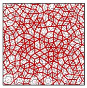
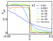
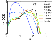
Figure 1: (color online) Left: Shadow system for a brownian system composed of soft harmonic spheres slightly above jamming at $\phi=0.86$ and $kT=10^{-8}$. The contacts are plotted with widths proportional to their effective stiffness $k_{\text{eff}}$, red with positive $k_{\text{eff}}$ and blue with negative $k_{\text{eff}}$. Center: Dependence of the effective stiffnesses $k_{\text{eff}}$ on the interparticle gap for different temperatures $kT$ and $\phi=0.86$; compare to the step function for the harmonic potential set in the simulation. Right: Density of states $D(\omega)$ computed from the eigenspectrum of ${\bf C_{p}\,}$for the same range of temperatures, compared to the one derived from the Hessian of the soft sphere potential.

Let us define the shadow system explicitly. Suppose some experimental system of colloidal particles moving around a metastable configuration ${|r^{0}\rangle}$. Once computed the effective spring constants $k_{ij}^{\text{eff}}$ between particles from the empirical inverse stiffness matrix K ${}^{\text{eff}}=kT{\bf C_{p}}^{-1}$, the shadow system is defined as the Hamiltonian system of harmonic springs with stiffnesses $k_{ij}^{\text{eff}}$, strung between particles of mass $m$ sitting in the metastable configuration ${|r^{0}\rangle}$. Note that the shadow system must not be confused with the model system the physicist has in mind when discussing his observations on the experimental system. In the present case, despite possible complicated electrostatic and hydrodynamic interactions, the colloidal system is considered as a good experimental realization of over-damped soft spheres in a thermal bath - the model system the physicist has in mind. Whereas the model system obeys an overdamped dynamics, the shadow system obeys the Hamiltonian dynamics of perfectly harmonic springs.

For thermal systems at equilibrium, the spectrum of ${\bf C_{p}\,}$can be interpreted as the vibrational modes of the shadow system and both the shadow system and the model system share the same density of states. However one must remember that the vibrational properties of the model system are still different from those of the shadow system. First, even in the linear regime, it is well known that resonance frequencies of a system of springs are shifted by damping and eventually completely eliminated in the over-damped limit. Second, the model system may well escape the linear regime. This is what happens for frictionless disks close to jamming, because of the vanishing range of linear response, as was shown recently Schreck et al. (2011). In the following we illustrate this last remark with two computational “experimental systems”. The first system consists of poly-disperse packings of thermal frictionless soft spheres interacting through a harmonic potential, and simulated with over-damped Langevin dynamics Allen and Tildesley (1999) close to the jamming transition. The second one consists of thermal hard sphere packings simulated with event-driven Newtonian molecular dynamics just below the jamming transition. Initial states are obtained by shrinking simulated packings at jamming by a factor $\delta\in[10^{-6}-10^{-2}]$ which controls the distance from jamming Brito and Wyart (2006).

Figure 1 displays the effective stiffnesses obtained for the soft sphere simulations slightly above jamming, at a very low temperature. We find effective stiffnesses consistent with the original connectivity and the original stiffness, which is a constant, here set to $1$ for the harmonic potential. The only exceptions are occasional weak interactions with cage neighbors which are not contacts. As can be seen in Figure 1 center, at low temperatures, the stiffness as a function of overlap remains close to the $T=0$ step function. At low temperatures, as one would have expected for soft spheres above jamming, the shadow system is reasonably close to the “experimental” one. As a result the density of states D $(\omega)$ computed from the Hessian matrix and the one computed from the spectrum of ${\bf C_{p}\,}$closely match (see figure 1, right).

When the temperature is increased, still remaining deeply within the glassy regime, we find that the stiffness as a function of the overlap broadens away from the $T=0$ step function, see Figure 1 bottom left. Equally, we find that the density of states obtained from ${\bf C_{p}\,}$begins to differ substantially from the Hessian density of states. The larger temperatures allow the system to explore the potential beyond the range of linear response.

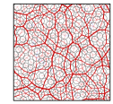
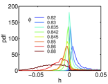
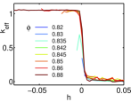
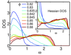
Figure 2: Top Left: Shadow system for a packing of thermal soft sphere just below jamming at $\phi=0.835$ and $kT=10^{-6}$. The contacts are plotted with widths proportional to their effective stiffness $k_{\text{eff}}$, red with positive $k_{\text{eff}}$ and blue with negative $k_{\text{eff}}$. Top right: interparticle gap distribution for a range of packing fractions; with a negative mean gap above jamming and a positive gap below jamming. Bottom left: Dependence of the effective stiffnesses $k_{\text{eff}}$ on the interparticle gap for different $\phi$; the different densities sample different regions of the stiffness curve. Bottom right: Density of states $D(\omega)$ computed from the eigenspectrum of ${\bf C_{p}\,}$compared to the one derived from the Hessian of the soft sphere potential with an added log-potential (inset; see text). All curves for $kT=10^{-6}$.

The differences between the shadow system and the model system become strongly apparent if we cross the jamming transition at finite temperature. Figure  2 shows different aspects of the shadow system as a function of packing fraction $\phi$ at finite (low) temperature $kT=10^{-6}$. From the plot of the shadow system at $\phi=0.835$, it is clear that the stiffnesses now deviate significantly from a step function. The gap distribution (top right) moves from distributions with only negative gaps (overlaps) above jamming, to a situation with only positive gaps below jamming. Around jamming, we find both over- and underlaps within the same packing, and both contribute to the effective stiffness. Even though the stiffness-gap function has only slightly broadened from a step function, the different packing fractions sample different parts of the curve (bottom left), and the resulting shadow system is significantly different from the model system. At high densities, we do recover a shadow system density of states which resembles the Hessian of the soft sphere potential (bottom right, compare to inset). At lower densities, the similarity breaks down, most clearly below jamming, where the soft sphere density of states has a large number of zero modes, and it is mechanically unstable, unlike the shadow system one.

In the inset to the bottom right figure, we compare the shadow system density of states to the simplest effective model for thermal soft spheres: $V_{eff}=V_{harm}+kTV_{log}$, that is we have added an effective logarithmic potential for hard spheres to the soft sphere potential (see below for a disscussion of the log-potential). While $V_{eff}$ captures part of the shift of the density of states to lower frequencies below jamming, it is not a good fit: all the shadow system density of states have a peak at intermediate frequencies, unlike the density of states obtained through $V_{eff}$.

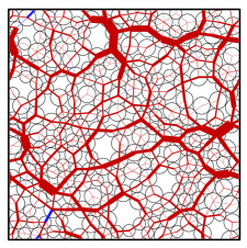
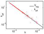
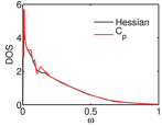
Figure 3: Top: Shadow system for a packing of $N=256$ thermal hard spheres just below jamming ($\phi=0.83878$, $\phi_{J}=0.83894$). The contacts are plotted with widths proportional to their effective stiffness $k_{\text{eff}}$, red with positive $k_{\text{eff}}$ and blue with negative $k_{\text{eff}}$. Bottom Left: effective stiffnesses as a function of the gaps separating the particles: in black the effective stiffnesses derived from the effective logarithmic potential; in red those extracted from the inversion of ${\bf C_{p}\,}$. Bottom right : Density of states $D(\omega)$ computed from the eigenspectrum of ${\bf C_{p}\,}$compared to the one derived from the Hessian of the effective potential.

The effective log-potential we just used was first introduced for hard spheres slightly below jamming where the situation is again not so clear: the hard spheres potential is singular and, as for the soft spheres case, the system is a priori not mechanically stable anymore. On one hand one can derive an effective pair potential and effective stiffnesses by computing the forces amongst the particles via the exchange of momentum during the collisions Brito and Wyart (2006). This potential scales like the logarithm of the interparticle gap. On the other hand, one can compute the effective stiffnesses derived from the inversion of ${\bf C_{p}\,}$. Figure 3 compares both effective stiffnesses for a system of $N=256$ hard disks just below jamming ($\phi=0.83878$, $\phi_{J}=0.83894$). We indeed find an effective connectivity of the packing even though in their mean positions, the particles are not touching. This is consistent with the effective potential approach and we also find $k_{\text{eff}}\sim 1/h^{2}$, where $h$ is the interparticle gap, consistent with a logarithmic potential. Hence the shadow system remains a good approximation in this case too. As a consequence one can again compare the density of state $D(\omega)$ computed from ${\bf C_{p}\,}$and the one derived from the Hessian of the effective potential. One observes on figure 3 that they match pretty well. Given the singular character of the hard sphere potential and the fact that the reference state is only a metastable state, this is a non trivial result which validates in a self consistent way both the approach in terms of an effective potential introduced in Brito and Wyart (2006) and the use of ${\bf C_{p}\,}$as a tool for extracting the density of states for slightly unjammed systems.

Before closing this section, let us mention that we have followed the same analysis in the case of a real experimental system composed of NIPA colloidal particles above jamming Chen et al. (2010). Conceptually, it is very similar to the soft sphere simulation we have just discussed. However, as already mentioned, the presence of a solvent and electrostatic interactions could alter the description in terms of a simple repulsive pair potential. We found that the effective stiffness is far above the noise for adjacent particles only. This tells us that elastic interactions between neighboring particles dominate the data, as they should. Furthermore, the effective stiffnesses as a function of the interparticle separation could be measured and is compatible with an harmonic or Herzian interaction. Hence also here the shadow system captures the essence of the vibrational properties of the real system under consideration. The reader interested by this experimental study should refer to the original paper.

III.2 Principal component analysis

So far we have discussed how to interpret the eigenmodes and eigenvalues of ${\bf C_{p}\,}$for thermally equilibrated systems. We have seen in section II.2 that for non equilibrium systems, the distribution of the energy on each mode must be known before extracting the density of state. This in general is not the case. However the spectrum of ${\bf C_{p}\,}$and the associated modes still convey a lot of information about the dominant modes of relaxations.

Such a path has been followed in analyzing different systems for which the underlying microscopic dynamics is unknown. In Laloux et al. (1999), the price fluctuations in financial markets are analyzed by comparing the spectrum of eigenvalues of the covariance matrix with the results of random matrix theory. The deviations from the purely random case contains the true information about the prices. In Micheletti et al. (2004) the protein near-native motion is characterized. Although molecular dynamics simulations based on all-atom potential allows the identification of a protein functional motion on a wide range of timescales, the very large time scales are not easily accessible in simulations. A way to bypass this problem is to study the correlations of the fluctuations of the deviation of the protein backbone from its native configuration. The principal components of this matrix correspond to the collective modes of the protein which happen on larger time scales.

Two of the present authors have used a similar approach in the case of vibrated granular media Brito et al. (2010). The experimental system consists in a 1:1 bidisperse monolayer of brass cylinders. Mechanical energy is injected in the bulk of the system by horizontally vibrating the glass plate on which the grains stand and dissipated by solid friction. The experimental protocol produces very dense steady states with a packing fraction up to $\phi=0.8457$. The stroboscopic motion of a set of $1500$ grains is tracked in the center of the sample. The set-up, the quench protocols and the main properties of the system, are described in detail in Lechenault et al. (2008a, b).

We now briefly illustrate the methodology adapted in Brito et al. (2010) to discuss the spectral properties of ${\bf C_{p}\,}$. We have considered a subset of $N=350$ grains acquired during $T=100$ time steps at a packing fraction $\Phi=0.844$ so that the metastable state of reference is well defined (no rattler, no structural rearrangement). Because $r=dN/T$, where $d$ is the space dimension, is larger than one, strictly zero eigenvalues appear in the spectrum of ${\bf C_{p}\,}$. We shall come back to this practical issue in the next section and restrict the discussion to the positive eigenvalues. The fluctuations of each grain $i$ around its metastable position are Gaussian but the width, $\sigma_{i}$, of the distribution is widely distributed amongst the particles. according to the fat tail distribution $\rho(\sigma)\sim\sigma^{-(1+\mu)}$ plotted on figure 4-top-left , where $\mu\approx 6$.

The Marc̆enko-Pastur theorem, the purpose of which is to relate the spectrum computed at finite $r$ to the one of the true correlation matrix could be used to obtain predictions but no explicit analytic form for the shape of the eigenvalue spectrum of ${\bf C_{p}\,}$. Please see appendix  VII.4 for details. One alternative strategy is to define a Random Model of uncorrelated Gaussian variables the width $\sigma_{i}$ of which are the experimental ones. We will refer to this model as the $RM_{\sigma}$ case. The eigenmodes extracted from the real dynamics with eigenvalues larger than the largest one of the $RM_{\sigma}$ model contain the relevant information about the correlations.

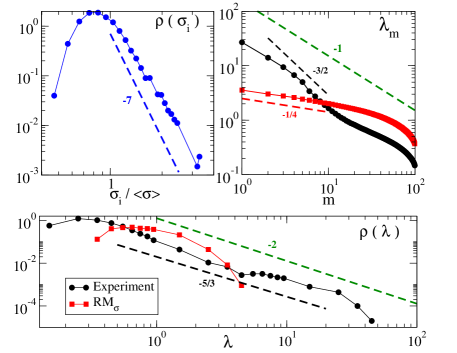
Figure 4: Eigenvalues of ${\bf C_{p}\,}$for jammed grains under horizontal vibration above jamming. Top-left : Probability density of the rms displacement of each grain around it average position in the metastable state. Top-right : positive eigenvalues sorted in decreasing order. Bottom : probability density of the positive eigenvalues. On the center and right plots the black dots correspond to the real dynamics and the red square to the $RM_{\sigma}$ model; the dotted line correspond to the expected distribution for a crystal according to the Debye law

.

Figure 4-top-right, respectively figure 4-bottom, displays the eigenvalues $\lambda_{m}$ sorted in decreasing order, respectively the probability density $\rho(\lambda)$ extracted from the real dynamics as compared to those obtained for the $RM_{\sigma}$ model. Note that there is a straightforward correspondence between these two curves since $\frac{1}{N}m(\lambda)$ is exactly the inverse cumulated distribution of $\lambda$ and a power-law behavior $\lambda_{m}\sim m^{-1/\alpha}$ translates into a density $\rho(\lambda)\sim\lambda^{-(1+\alpha)}$. The five largest eigenvalues for the experimental system are clearly larger than the largest one obtained for the $RM_{\sigma}$ model. This comparison shows unambiguously that the top eigenvalues of ${\bf C_{p}\,}$contain useful information about the dynamics of the system, and are not drowned in noise. It also demonstrates the existence of strong spatial correlations: by moving together, particles achieve large collective fluctuations that would not develop otherwise.

If one should not try to convert these eigenspectrum into density of states, it is however always possible to convert the expected density of states of a thermal crystal into the the spectrum of its dynamical matrix. Here, a 2d crystal, with a density of states $\rho(\omega)\sim\omega^{d-1}=\omega$, with $\omega\propto\lambda^{1/2}$, has $\rho(\lambda)\sim\lambda^{-2}$, that is $\alpha=1$ and $\lambda_{m}\sim m^{-1}$ as indicated on the figures by the green dotted line. The experimental data are consistent with an estimated $\alpha\approx 2/3$, that is a slower decay of the spectrum than for the crystal case. One can interpret this result saying that there is a larger fraction of modes participating in the dynamics than in the crystalline case.

One can also analyze the structure of the most significant modes. This was done in Brito et al. (2010) for this system of bi-disperse grains when approaching jamming from above, and it could be demonstrated quantitatively that there is a redistribution of spectral weight towards larger eigenvalues corresponding to softer modes and that the softest mode becomes more coherent and spatially organized. However, as it was discussed above, for such a system where the energy is not distributed evenly over the modes, one cannot convert this information into the vibrational properties and the density of states of the system. The results presented here as well as in Brito et al. (2010) illustrate well how the PCA of the dynamics remains a fruitful tool of analysis without referring to the vibrational properties.

IV Practical guideline

In the previous section, we have assumed that the data at hands were “perfect”in the sense that neither statistical limitations nor resolution issues came into play. Also we did not consider the possibility of a strong anharmonicity of the dynamics and we have not discussed the way, one should get rid of the rattlers, those particles which do not participate in the collective motion but instead “rattle” in their cages.

Measuring ${\bf C_{p}\,}$to a sufficient level of precision to extract reliable information from it is not a simple affair. The goal of this section is to disentangle all the possible sources of practical problems that one faces when computing ${\bf C_{p}\,}$and to propose methods and alternatives to obtain a faithful information from its spectrum.

In subsection IV.1, we start by discussing a way to test the metastability of the reference state. Indeed all the approach is based on the fact the displacement field is purely composed of vibration around a steady reference state. We illustrate this issue in the case of hard spheres, which by definition sit below jamming, where metastable states only have a finite lifetime. It is thus of crucial importance to control that the system does not escape the metastable state during the time window of the analysis. In subsection IV.2, we then illustrate on the case of vibrated granular media, how one can observe anhamonicity setting in when approaching the jamming transition from above. The reader may also refer to Schreck et al. (2011), where the same issue is discussed in the case of numerical simulations of soft spheres. As an immediate consequence of the above effects, the time window of the analysis may be seriously shortened as compared to the full duration of the numerical or real experiment. Hence statistical issues come into play. More specifically, we shall see in sections IV.3 and  IV.4 how to deal with statistical independence of the data as well as convergence issues. In the case where the data sets have been obtained experimentally, resolution issues may also alter the analysis. We thus consider in subsection IV.5 a NIPA colloidal experiments to illustrate how convergence and experimental resolution interplay to affect the computation of the density of states. Finally, identifying rattlers is usually a challenging matter. It emerges that calculating the eigenspectrum itself is a good “filter” for rattlers: their motion appears only in a few low energy eigenvalues which do not mix with the remainder of the motion. This is discussed in section IV.6.

IV.1 Metastability

Before starting any of the analysis discussed in the previous section, one must have checked that the dynamics is purely composed of fluctuations around a well defined reference state. This can be done both a priori, in order to select a good time window to perform the analysis, and a posteriori on the basis of the properties of ${\bf C_{p}\,}$. A natural tool to characterize the dynamics is the self-intermediate correlation function, defined as

$$C_{q}(t_{0},t)=\langle~{}\cos(\vec{q}~{}.\Delta\vec{r}_{i}(t,t_{0})~{}\rangle_{j},$$ (16)

where the average is made on the particles but not on the initial time. $\Delta\vec{r}_{i}(t,t_{0})=\vec{r}_{j}(t)-\vec{r}_{j}(t_{0})$ is the displacement of the particle $j$ between $t_{0}$ and $t+t_{0}$, $\vec{q}$ is a vector whose amplitude is given by $q=\pi/a$ and $a$ is a length scale which sets the amplitude of the displacement above which the particle motion induces a change of metastable state. There is obviously a large part of arbitrariness in such a definition and traditionally $a$ is set to a fraction of the particles diameter, so that a metastable state more or less corresponds to a given configuration of neighbors.

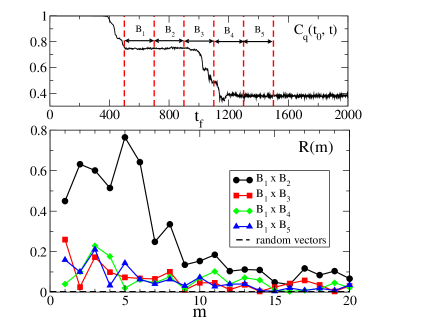
Figure 5: Probing metastability. Top : $C_{q}(t_{0},t)$ for a system of hard spheres below jamming ($N=1024$ and $\phi=0.841947$; $\phi_{J}=0.841959$). The time unit is $t_{f}$, the time interval at which particle positions are stored, and corresponds to $800$ collisions per particle. Each interval delimited by dashed lines has $200$ snapshots, during which we compute ${\bf C_{p}\,}$and its basis $B_{i}$ of eigenvectors $\{|\lambda_{m}\rangle\}$. Bottom : Robustness of the first $20$ modes as defined in Eq.(17) between pairs of intervals $B_{i}\times B_{j}$ as indicated in the legend. The dashed line indicates the value of $R(m)$ for purely random eigenvectors.

Figure 5-top displays $C_{q}(t_{0},t)$ computed for a system of $N=1024$ bidisperse hard discs the dynamics of which has been simulated using molecular dynamics slightly below jamming ($\phi=0.841947$; $\phi_{J}=0.841959$)  Brito and Wyart (2006, 2007). Here $a$ has been set to the radius of the smaller particles. One observes very well defined plateaus, during which the system is trapped in a metastable state, separated by a quick relaxation event that we call crack. Typically, the size of the plateau defines $T$, the interval of time available to compute ${\bf C_{p}\,}$. There are however some cases where one cannot identify the plateaus so easily. As a matter of fact this will happen each time the system size is large as compared to the typical size of a crack. When this is the case, one can always cut the system into smaller subsystems and do the analysis in each subsystem as illustrated in Brito et al. (2010).

As long as the system remains in the same state of reference, the basis of eigenvectors should essentially remain unchanged. This can be checked by dividing the time interval of duration $T$ in smaller subintervals and computing an indicator of the modes robustness, defined as Brito et al. (2010):

$$R(m)=\sum_{j=-M}^{j=+M}\langle\lambda_{m}|\lambda^{\prime}_{m+j}\rangle^{2},$$ (17)

where $\langle\lambda_{m}|\lambda^{\prime}_{m+j}\rangle$ is the scalar product between the modes computed during two successive observation windows of duration $T^{\prime}<T$. Setting $M$ to a small but strictly positive value allows neighboring modes to possibly exchange their rank. As long as the largest eigenvalues are concerned, we could check that the results are basically independent of $M$ for $M\geq 2$ and we fixed $M=2$. Figure 5-bottom displays $R(m)$ for the twenty largest eigenvalues computed between intervals defined as indicated on figure 5-top by vertical dashed lines. The robustness of the the first modes is higher when computed amongst intervals belonging to the same plateau. As soon as one compute the modes on an interval including the crack, the robustness decreases sharply and rapidly reaches the baseline level $R(m)=(2M+1)/2N$, one would obtained for purely random vectors. Note also that the robustness is not restored when the two intervals belong to different plateaus indicating that the system has indeed relaxed from one metastable state to another.

IV.2 Harmonicity of the dynamics

In the previous section, we have identified a metastable state and checked a posteriori that the basis of eigenvectors remains unchanged during the lifetime of this state. As a matter of fact, one must also check that the dynamics around this state is purely harmonic. For an equilibrium system close to jamming, the structure of the packing is frozen and fluctuations of the particles are thermal, so that assuming Gaussian fluctuations around the metastable state sounds reasonable. However it was recently claimed that repulsive contact interactions make jammed particles systems inherently anharmonic Schreck et al. (2011). The authors argue that at very low temperature the breaking and forming of inter-particles contact is responsible for anharmonicity in the sense that the response does not remain confine to the original mode of excitation. Such a definition of harmonicity is very strict, and how the result depends on system size, temperature and distance to jamming is still a matter of debate. It is clear that for mechanically excited athermal and dissipative systems, such as shaken macroscopic grains, there is no reason why the dynamics should be harmonic.

While studying horizontally shaken grains, two of the present authors proposed to check the harmonicity of the dynamics in a naive but experimentally accessible way, namely by computing the distribution of the individual fluctuations: $\rho(\delta x_{i}/\sigma_{i})$, where $\delta x_{i}$ is the position fluctuation along a given direction and $\sigma_{i}$ is the root mean square displacement of particle $i$. Figure 6 presents such distributions obtained for a system of $N=1550$ brass disks shaken horizontally on a oscillating plate just above jamming ($\phi_{J}=0.8417$, see Lechenault et al. (2008a) for details on the experimental set up and protocol). The distributions are computed for four different packing fractions $\phi$ and four durations $T$ of the window of observation. They are then ensemble averaged over the $10^{4}/T$ intervals provided by the full dataset.

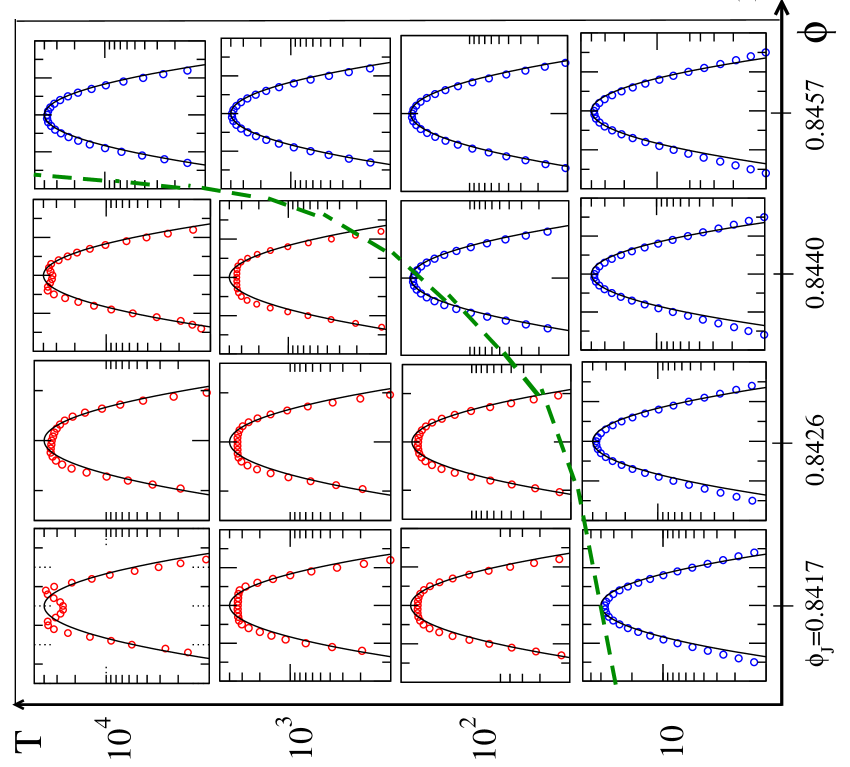
Figure 6: Distributions of the position fluctuations $\rho(\delta x_{i}/\sigma_{i})$ for four values of the packing fraction and four durations of observation $T$. We focus on the top of the distribution, which is compared to a Gaussian (continuous black line). The green hatched line separates the distributions well described by a Gaussian from those deviating from this harmonic description

The distributions shown in figure 6 highlight some important characteristics of the dynamics. The parameter space $(\phi,T)$ can be divided into two regions, as illustrated by the green hatched line: for small enough observation duration $T$ or large enough packing fractions, the distributions are unimodal with a Gaussian core: particles jiggle around a well defined average position; for longer $T$ or smaller densities, the distribution starts developing a flat top, with a poorly defined maximum. This suggest that on these longer observation times, the average position of a significant part of the particles is not well defined anymore. Particles either drift slowly or even find (collectively) another metastable position, as suggested by the double peak observed in the case $\phi=0.8417$ and $T=10^{4}$, i.e. for the loosest packing fraction and the longest observation time. This means that over long time scales, the evolution of the average position becomes comparable or even larger than the fluctuations, and it becomes meaningless to describe the system in terms of small vibrations around a fixed metastable state. For an infinite size system, some rearrangement always happens somewhere, and the covariance matrix ${\bf C}_{p}$ is always ill-defined. The “allowed” time scale $T_{\max}(\phi,L)$ is expected to scale inversely with the system size $L$.

IV.3 Statistical independence

Once a reference state is identified during a time window of duration $T$, one needs to know whether the particle positions stored on successive snapshots are independent, or at least sufficiently uncorrelated to compute ${\bf C_{p}\,}$. Again computing the robustness of the basis of eigenmodes is a good way to check the validity of the analysis: if the particle positions are not independent the correlator ${\bf C_{p}\,}$is badly estimated and the eigenmodes are mostly composed of noise. To illustrate this point we use again the hard discs system just below jamming ($\phi=0.83878$; $\phi_{J}=0.838865$), now with $N=256$, for which we could identify a long lasting metastable state the total duration of which, $T$, corresponds to $1.6\times 10^{6}$ collisions per particles.

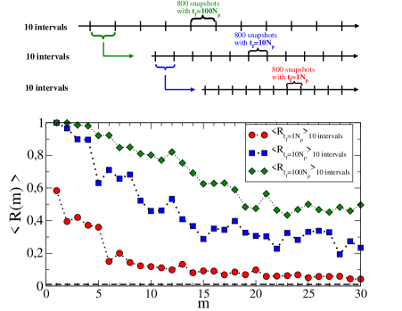
Figure 7: Testing statistical independence during a given metastable state for a system of $N=256$ hard disks below jamming ($\phi=0.83878$; $\phi_{J}=0.838865$). Top : sketch of the time discretization procedure (see text for details). Bottom : $\langle R(m)\rangle$ for the three discretization scheme as indicated by the legend.

Figure 7-top sketches the procedure. The total acquisition is divided in $10$ intervals. Each of them contains $800$ snapshots of the positions, separated by $t_{f}=200$ collisions per particle. ${\bf C_{p}\,}$is computed and diagonalized on each interval, and the average robustness among successive intervals $\langle R(m)\rangle$ is evaluated for the first $20$ largest eigenvalues. To preserve the same statistics, together with a reduced interval of time between the snapshots, we then subdivide each interval in $10$ subintervals, each of them containing again $800$ snapshots of the positions, but now separated by $t_{f}=20$ collisions per particle. And the procedure is iterated once more leading to $800$ snapshots of the positions separated by $t_{f}=2$ collisions per particle in each interval. Figure 7-bottom compares $\langle R(m)\rangle$ for the three successive level of time discretization. Although the system remains in the same metastable state, the number of snapshots and the averaging used to compute ${\bf C_{p}\,}$are identical in all three cases, one clearly observes the convergence of $\langle R(m)\rangle$ towards larger values when the snapshots are well separated. In the present case the finest discretization is obviously irrelevant and a separation of successive snapshots larger then about $50$ collisions per particle is necessary.

Altogether, whether it comes from experimental limitations of the acquisition rate or from a microscopic timescale inherent to the dynamics, there is always a minimal timescale separating the accessible and useful snapshots of the particle positions. Since we have also seen that the analysis is confined to the lifetime of the reference state, we are now in the position to face the convergence issue of the eigenspectrum as discussed by the Marc̆enko Pastur theorem.

IV.4 Convergence of the spectrum (small sample limit)

The Marc̆enko-Pastur (M-P) theorem Marc̆enko and Pastur (1967); Silberstein and Bai (1995); Karoui (2008); Laloux et al. (1999) applies to the ensemble of Wishart random matrices; that is the ensemble of $p\times p$-matrices constructed by the addition of $n$ independent samples $x_{i}x_{j}$, where the $x_{i}$ ($i\in 1...p$) are distributed according to either a multivariate Gaussian distribution or a distribution with finite higher moments, similar to the conditions of the central limit theorem. The M-P theorem then predicts the eigenvalue distribution of such matrices in the limit $n\rightarrow\infty$, $p\rightarrow\infty$, $r=p/n$ finite. However, as one can see in appendix VII.4, there is no explicit form for the distribution. Also, the theorem tells nothing about the convergence of the eigenmodes. This is why we concentrate here on the numerical characterization of the convergence in a specific and well controlled situation. This will allow us to discuss both the shape of the spectrum and the relevance of the modes themselves. Also, it will allow us to examine the case where $r>1$, when a finite part of the spectrum is strictly zero. The reader interested in analytical predictions may refer to the original papers  Marc̆enko and Pastur (1967); Silberstein and Bai (1995); Karoui (2008); Laloux et al. (1999), as well as to appendix VII.4.

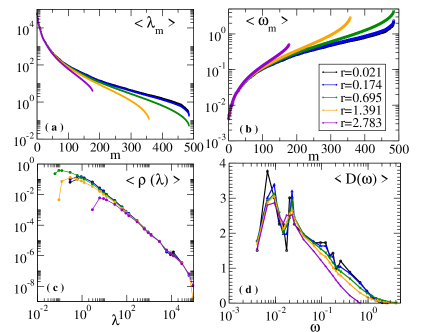
Figure 8: Convergence of the spectrum of eigenvalues of ${\bf C_{p}\,}$for a system of $N=256$ hard disks below jamming ($\phi=0.83878$; $\phi_{J}=0.838865$) for decreasing values of $r=2N/n$ as indicated in the legend. Top: Eigenvalues (left) and corresponding eigenfrequencies (right) sorted in decreasing, respectively increasing order. Bottom: Eigenvalues spectra (left) and corresponding density of states (right).

We consider the same system as above, with $N=256$ hard disks just below jamming ($\phi=0.83878$; $\phi_{J}=0.838865$) within a long lasting metastable state of total duration $T=4.6\,10^{6}$ collisions per particles and we choose to retain as independent particle positions separated by $200$ collisions per particle, so that $n=23000$. In section III.1, we have shown that the spectrum of ${\bf C_{p}\,}$and that of the effective dynamical matrix match when the whole set of data is used to compute ${\bf C_{p}\,}$. Here we discuss how much the spectrum and the modes of ${\bf C_{p}\,}$deviate from their asymptotic behavior when the time interval used to compute ${\bf C_{p}\,}$is artificially reduced such that $r=2N/n$ varies in the range $[0.021-2.28]$.

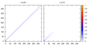
Figure 9: Matrices of the scalar product between the modes of ${\bf C_{p}\,}$and the modes of the dynamical matrix for a system of $N=256$ hard disks below jamming ($\phi=0.83878$; $\phi_{J}=0.838865$). The rows are the indices of the modes in increasing order of their frequency and the colorbar indicates the value of the scalar product. Left: $r=2N/n=0.021$ Right: $r=2N/n=2.78$.

Figure 8 displays the spectral properties of ${\bf C_{p}\,}$for increasing values of $r$. As soon as $r>0.5$, the smallest eigenvalues are seriously underestimated, respectively the largest frequencies are overestimated. For $r>1$, strictly zero eigenvalues replace the lowest eigenvalues. On the contrary, the largest eigenvalues, respectively the lowest eigenfrequencies, are surprisingly robust, even in the cases $r>1$. Because of this robustness, when one is interested in the low frequency part of the density of states, it is recommended to normalize the density such that the area under the curve equals the fraction of non-zero eigenvalues. As a result, the density of states $D(\omega)$ conserves its shape as long as $r<1.5$ and only for larger $r$ the large frequencies part of the density of states starts to be significantly depleted.

Finally figure 9 illustrates the robustness of the modes themselves. To do so, we define the matrix of scalar product between the two eigenbasis: the modes of ${\bf C_{p}\,}$and the modes of the effective dynamical matrix. If the modes were strictly the same, this matrix should be the identity matrix. Figure 9-left shows the matrix of the scalar products for $r=0.021$, from where we observe that the modes of ${\bf C_{p}\,}$project on a very small number of modes of the effective dynamical matrix, as already pointed at in section III.1. We see that even for $r=2.78$, the modes of ${\bf C_{p}\,}$associated with the largest eigenvalues still project on a small number of modes of the effective dynamical matrix, while the modes of ${\bf C_{p}\,}$with a higher frequency are spread across the whole spectrum of the effective dynamical matrix.

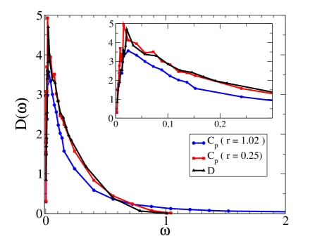
Figure 10: Density of states for a system of hard disks below jamming ($\phi=0.841947$; $\phi_{J}=0.841959$) extracted from ${\bf C_{p}\,}$either computed using the whole system of $N=1024$ hard disks (in blue) or cutting the system in 4 sub-systems with $N_{p}^{sub}=256$ each (in red) as compared to the density of states obtained from the effective dynamical matrix computed for the whole system (in black). Inset: zoom on the lowest frequency part of the density of states.

Altogether, as long as $r<1.5$, the most significant eigenmodes and eigenvalues of the dynamic matrix as well as the qualitative features of the density of states are well captured by the analysis of ${\bf C_{p}\,}$. Practically speaking, when very long lasting metastable states are available it is thus often advantageous to average the spectrum or the density of states on successive time windows, provided that the duration of each of them satisfies $r\approx 1$.

When there is no enough snapshots to recover the whole spectrum of modes, an alternative strategy is to reduce the system size in order to increase $r$. In principle one can divide the system in smaller subsystems, and compute the density of states in each of them. This strategy allows to better access the low frequency part of the density of states, although the lowest accessible frequency increases as the inverse of the system size. Figure 10 and figure 11 illustrate the application of such a strategy to a system of $N=1024$ particles below jamming ($\phi=0.841947$; $\phi_{J}=0.841959$). In this example, the metastable state has a total duration of $T=1.6\times 10^{5}$ collisions per particles and we store independent particle positions separated by $80$ collisions per particle. This means that $n=2000$ snapshots and $r=1.02$. From figure 8 we know that for this value of $r$ the large frequencies are underestimated. By cutting the system in 4 boxes, each one has $r=0.25$ and we are now able to recover the whole spectrum. In figure 10 we compare the density of states $D(\omega)$ extracted from ${\bf C_{p}\,}$either using the whole system of $N=1024$ hard disks $(r=1.02)$ or cutting the system in 4 sub-systems with $N_{p}^{sub}=256$ each $(r=0.25)$ to the density of states obtained from the effective dynamical matrix computed for the whole system. Whereas the spectrum obtained from ${\bf C_{p}\,}$computed with the whole system only captures the very low frequencies, the one computed for the sub-systems matches the spectrum from the dynamical matrix on the whole range of frequencies.

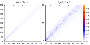
Figure 11: Matrices of the scalar products between the modes of ${\bf C_{p}\,}$and the modes of the dynamical matrix for a system of $N=1024$ hard disks below jamming. Left: Modes of ${\bf C_{p}\,}$computed on the whole system. Right: Modes of ${\bf C_{p}\,}$reconstructed from the modes computed separately in four sub-systems of size $N_{p}^{s}ub=256$. The horizontal (resp. the vertical) indices label the modes of the dynamical (reps. the covariance) matrix. The color bar indicates the value of the scalar product.

Concerning the robustness of the modes, once the modes have been computed in each subsystem, we first reconstruct artificial modes for the whole system by pasting together the modes of each subsystem. Note that the number of modes in these 2 basis is not the same: for the whole system there are $2N_{p}=2048$ modes while in each subsystem has $2N_{p}^{sub}=512$ modes. Figure 11 shows the matrices of the scalar products between the modes of the dynamical matrix and those of ${\bf C_{p}\,}$, either computed on the whole system (left) or reconstructed as described above from the modes computed on the subsystems (right). Despite the artificial nature of the modes obtained from the computation of ${\bf C_{p}\,}$in each subsystem, their projection on the modes of the dynamical matrix remains rather concentrated, especially when one remembers that each mode of ${\bf C_{p}\,}$in this case projects approximately on four modes of the dynamical matrix.

Let us end this section by quoting a recent work Schindler and Maggs (2011) which shows that in general the modes are modified by the truncation of the full real-space correlations and proposes windowing strategies to best avoid these boundary conditions artifacts. Implementing such strategies on top of the segmentation proposed here would certainly deserve proper attention.

IV.5 Convergence and experimental resolution (large sample limit)

Even in the most favorable case of all experimental situations discussed above, we have not yet addressed the issue of the experimental resolution. As detailed in appendix VII.4, the Marc̆enko-Pastur theorem allows us to compute the impact of a finite resolution on the spectral properties of ${\bf C_{p}\,}$at a finite $r=2N/n$, where $n$ is again the number of independent snapshots of the particle positions.

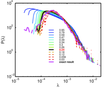
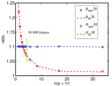
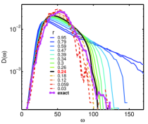
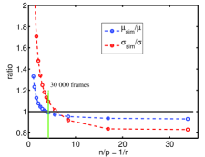
Figure 12: Statistical convergence analysis for the NIPA system Chen et al. (2010), using the ‘random vector’ model (see text). Top left: Numerical eigenvalue distribution for different values of $r$ as indicated in the legend. The distribution associated with the experimental value $r=0.24$ is plotted in black and the asymptotic $r\rightarrow 0$ one is plotted in pink. Bottom left: Same for the density of states. Top right: Numerical (dots, subscript ‘sim’) and theoretical (dashed lines, subscript ‘th’) results for the mean and variance of $P(\lambda)$ normalized by the exact result. The experimental value of $r=0.24$ is indicated by a green line. Bottom right: Same for the density of states, numerical result only (dots and dashed lines, subscript ‘sim’). The green line marked ‘30 000 frames’ corresponds to the number of samples in the experimental NIPA system Chen et al. (2010).

To do so we assume that the applicability conditions of the theorem detailed in appendix VII.4 are met. The finite moments condition corresponds broadly speaking to a long-lived metastable state with short-time fluctuations of the particles in well-defined cages. The metastability condition can be tested through the methods of the section IV.1. For an equilibrium system, the short-time fluctuations of the particles in their cages are thermal and can hence well be approximated as gaussian within the range of linear response. For a non-equilibrium system such as shaken granular systems, this condition needs to be verified experimentally. The independence of the different samplings of the system can be tested through the methods of section IV.3.

If we have now constructed ${\bf C_{p}\,}$in these conditions, how does the experimental resolution affect the properties of the matrix and how does it interplay with the finiteness of $r$? How does it modify the spectral properties of the true correlation matrix, the one would obtain in the limits of infinite resolution and $r\rightarrow 0$? We model the resolution as an additive Gaussian noise of variance $\epsilon^{2}$, where $\epsilon$ is the resolution-induced uncertainty of the particle positions. If $C_{0}$ is the true correlation matrix, i.e. the one of the shadow system, one easily shows that for Gaussian fluctuations of the particle positions, the finite resolution correlation matrix is $\tilde{C}_{0}=C_{0}+\epsilon^{2}I$, where $I$ is the identity matrix. Then the measured ${\bf C_{p}\,}$is $\tilde{C}_{r}$, such that ${\rm lim}_{n\rightarrow\infty}\tilde{C}_{r}=\tilde{C}_{0}$. The Marc̆enko Pastur theorem is still valid and one finally relates the eigenvalues distribution of $\tilde{C}_{r}$ and the true correlation matrix $C_{0}$.

As for the case without noise, there is no explicit form for the distributions, but we show in appendix VII.4 that the mean and variance of the eigenvalue distribution of ${\bf C_{p}\,}$converge with $r\rightarrow 0$ and $\epsilon/\mu_{0}\rightarrow 0$ in the following way:

$$\tilde{\mu}_{r}=\mu_{0}+\epsilon^{2}$$

$$\tilde{\sigma}^{2}_{r}=\sigma^{2}_{0}+r\mu_{0}^{2}+r\epsilon^{4},$$ (18)

where the quantities labeled $0$ refer to the exact eigenvalue distribution and the ones labeled $r$ to the measured quantities. Note that for uncorrelated particles $\mu_{0}$, would be the typical cage size squared, i.e. the value of the plateau in the mean square displacement curves, preceding the onset of diffusive behavior. Interestingly, while the resolution directly impacts the mean, it only changes the width at $\mathcal{O}(\epsilon^{4})$, and the correction is moreover multiplied by $r$. As a result the noise dependence of the eigenvalue distribution is in fact much weaker than one might have expected.

We now present the results of a statistical model specifically developed to test the validity of the experimental results for colloidal NIPA particles Chen et al. (2010). In the experiment, $N=3600$ particles forming quasi two dimensional packings deep in the glassy phase were imaged with a confocal microscope, yielding $n=30000$ independent samples of their positions per run. In the language of the Marc̆enko-Pastur theorem, this corresponds to $r=0.24$. The combination of optical resolution and sub-pixel accuracy particle tracking led to an estimated uncertainty in the particle positions of $\epsilon=0.007\mu m$.

We build a ‘random vector’ model by constructing a model ${\bf C_{p}\,}$where we repeatedly sample from an uncorrelated multivariate normal distribution coresponding to the experimentally measured cages sizes, and with added noise at the experimental amplitude. The covariance matrix of the model is then $\tilde{C}_{ij}=(\lambda_{i}+\epsilon^{2})\delta_{ij}$, where the $\lambda_{i}$ are the diagonal elements of one of the measured ${\bf C_{p}\,}$from  Chen et al. (2010). While this model resembles the ‘Random Model’ introduced in section  III.2 detailing PCA, our aim here is different: we only intend to illustrate equation 18 with a model where we know the exact eigenvalue distribution in the absence of noise and for $r\rightarrow 0$. By construction, this is just $P(\lambda_{i})$, the distribution of diagonal elements or cage sizes which enter the model.

Figure 12 (top-left) shows the convergence of the numerical eigenvalue distribution $\tilde{P}_{r}(\lambda)$ as $r\rightarrow 0$ at fixed noise. The eigenvalue distribution corresponding to the experimental value $r=0.24$ is shown in black. It appears to be relatively close to the exact distribution shown in pink. The numerically obtained first two moments of the distributions exactly match the theoretical result from equation (18) (fig. 12(top-right). The curves ndicate that for the experimental value of $r$ (green vertical line), the error made compared to the true converged noiseless distribution is of the order of $10\%$.

For equilibrium systems, one is mostly interested in the density of states. Unfortunately, when performing the change of variables $\omega=\sqrt{k_{B}T/m\lambda}$, there is no straightforward and reliable way to calculate the moments of the distribution and we have to rely mostly on numerical results. Only the asymptotic values in the limit $r\rightarrow 0$ could be obtained (see appendix VII.4). In the bottom row of figure 12 we have applied the transformation $\omega=1/\sqrt{\lambda}$ numerically to obtain the density of states and its first two moments for the ‘random vector’ model. The density of states obtained for the experimental value of $r=0.24$ again matches pretty well the asymptotic one. Note that we find a fortitous compensation in the moments of the distributions: in the limit $r\rightarrow 0$, one can show that a finite resolution systematically leads to an underestimation of both the mean and the variance. Since working at finite $r$ always leads to an overestimation of these moments, it compensates the above underestimation. In the present case, the experimental value of $r$ (green line) is very close to the point where the compensation is perfect. Note that this is pure coincidence related to the specific values of the moments of the true distribution, and that even so it does not validate the detailed shape of the distribution.

In the case of the experimental data obtained with NIPA particles Chen et al. (2010), and for which correlations are present, the authors tested convergence of the density of states based on the methods outlined here and found scaling of mean and width consistent with our example. The error from experimental and statistical resolution was estimated in the $10\%$ range at $r=0.24$.

We can make a similar comparison for the hard sphere colloid setup of Ghosh et al. Ghosh et al. (2010). For this experiment, the estimated number of particles is $N=2000$, and approximately $n=4000$ samples at a resolution of $\epsilon=0.03\mu m$ were taken to obtain the DOS. While the resolution effect is comparable to the NIPA setup, we obtain $r\approx 1$. This introduces a large error into the measurement of the DOS, similar to the $r=0.95$ curves in the left panels of Figure 12. We estimate an error of $40\%$ and $200\%$ on the mean and the width of the DOS, respectively. However, as detailed in the previous section, even at this $r$ it is still possible to obtain the relevant low energy modes Ghosh et al. (2011).

IV.6 Rattlers

Close to jamming, there are few particles, the so called rattlers, which do no participate to the rigidity of the structure: removing them does not alter mechanical stability. When computing for instance the average coordination of the packing, these rattlers need to be identified and excluded. For simulations of soft spheres, the procedure is straightforward. The number of contact is known for each particle and those which have less than two contacts are considered as rattlers. For simulations of hard spheres just below jamming, the contacts are defined by computing the transfer of momentum during successive collisions. Again the particles with less than two contacts are defined as rattlers, but also those which have a significant smaller momentum transfer per contact as compared to the average. Such a criterion was proposed in Brito and Wyart (2009), where it was shown that particles with momentum transfer per contact smaller than $2\%$ of the average value could safely be considered as rattlers. Varying this threshold in the range $0.5-5\%$ did not alter the results.

We now offer an alternative way to identify rattlers in experiments by using the Principal Component Analysis (PCA) itself and compare it to the above method used for hard spheres. As a matter of fact, the PCA diagonalizes the dynamics on its dominant features. Since the rattlers are not tightly confined by their neighbors, they move significantly more than other particles. Also such motion are by definition localized on a single particle. Hence rattlers correspond to very singular kind of excitation and thereby tend to jeopardize the modes structure. Diagonalizing ${\bf C_{p}\,}$and analyzing the modes with high eigenvalues and a very high participation ratio is thus a good strategy to identify rattlers. Here the participation ratio of a given mode $m$ is simply defined as $P(m)=\sum_{i=1}^{N}(\delta r_{i}^{m})^{4}$, where $\delta r_{i}^{m}$ is the displacement of the particle $i$ on the mode $m$. Given that the modes are normalized, $\sum_{i=1}^{N}(\delta r_{i}^{m})^{2}=1$ so that a perfectly delocalized mode has a participation ratio of $1/N$, whereas a mode fully localized on a single particle would have a participation ratio of order one.

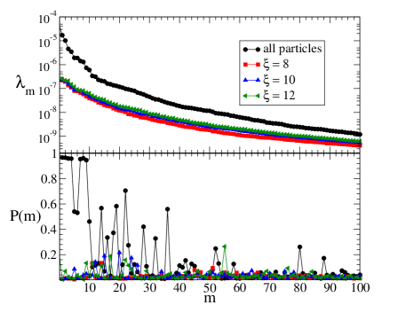
Figure 13: Eigenvalues of ${\bf C_{p}\,}$and participation ratio as defined in the text for a system of $N=256$ hard disks below jamming ($\phi=0.83878$; $\phi_{J}=0.838865$) with its rattlers (black curves) and having removed them according to different values of the thresholding criteria $\xi$ as indicated in legend. See text for the definition of $\xi$.

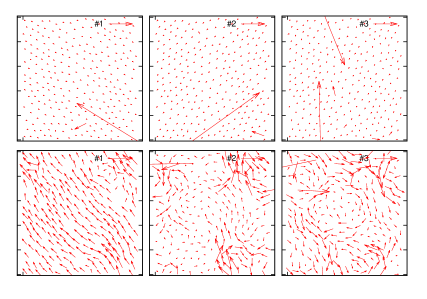
Figure 14: Eigen modes of ${\bf C_{p}\,}$for a system of $N=256$ hard disks below jamming ($\phi=0.83878$; $\phi_{J}=0.838865$) with its rattlers (top row) and having removed them (bottom row).

The method is illustrated in the case of a system of $N=256$ hard disks just below jamming ($\phi=0.83878$; $\phi_{J}=0.838865$) within a long lasting metastable state of total duration $T=4.6\times 10^{6}$ collisions per particles with $n=23000$ independent snapshots and $r=0.021$. Figure 13 shows the spectrum and the participation ratio of the modes of ${\bf C_{p}\,}$computed with and without rattlers. One easily identifies the modes with a simultaneously large eigenvalue and high participation ratio. Three of these modes are plotted on figure 14-top. Here also, one immediately identifies the rattlers with huge displacements as compared to the other particles. The rattlers in each modes are then defined as the particles having a displacement amplitude larger than $\xi$ times the average displacement inside the mode: $\delta r_{j}^{m}\geq\langle\delta r^{m}\rangle+\xi\sigma_{\delta r}^{m}$, with $\sigma_{\delta r}^{m}$ being the standard deviations of the displacement on the mode $m$. One must fix a threshold; however because the modes selected by the procedure concentrate most of the motion on the rattlers, it is very easy to fix the threshold and the results are robust to the choice of $\xi$, as it can verified in the figure 13. Once the rattlers are identified – sometime in several modes –, one eliminates them and recompute ${\bf C_{p}\,}$. One then easily checks that the extremely localized modes have disappeared, together with the rattlers, figure 14-bottom. Note that most of the particles identified as rattlers using this criterion are identical to those identified with the previous criterion used in Brito and Wyart (2009). The mismatch between both criteria is of the order of $10\%$ of the rattlers identified.

V Conclusions

We have reviewed various situations for which the study of ${\bf C_{p}\,}$, the covariance matrix of the positions of a system of particles can be used to infer dynamical properties of the system. It has been emphasized that for systems without equipartition of the energy, or without an independent knowledge of the energy repartition amongst the modes, the spectrum of ${\bf C_{p}\,}$cannot be transposed into the density of states of the system. Still, it conveys relevant informations about the dynamics and physicists would gain in exploring the path already followed. We have also insist on the physical interpretation of the modes obtained via the analysis in terms of the vibrational properties of the ‘shadow system’, which must not be confused with the experimental system, even an idealized one.

We then have seen the numerous steps one has to go through in implementing the analysis. Metastability of the reference state, harmonicity of the dynamics, statistical independence, convergence and experimental resolutions are all key elements to care of. How to deal with rattlers was finally discussed. Following the whole procedure requires as always a bit of physical insights, a good knowledge of the system of interest and patience. We have not discussed the new physics one can finally extract from the analysis. It certainly depends on the specificity of each system, but in any case one should remember that the analysis remains linear in essence.

We hope that in this light the present review of the methods associated to the correlation matrix approach will be useful to the community.

VI Acknowledgements

We would like to thank J.-P. Bouchaud and G. Biroli for inspiring the correlation matrix approach and pointing to the Marc̆enko-Pastur theorem and acknowledge the soft matter groups at U Penn for collaborating and sharing their data on the NIPA system. None of the present work would have been done without the numerous discussions, we have had at various level with those involved in the analysis in terms of vibrational modes of experimental and numerical data. In particular we thank Wouter Ellenbroek, Andrea Liu and Corey O’Hern for helpful discussions on the interpretation of modes. A special thought to Wim van Sarloos and Martin Van Hecke who hosted us in Leiden and always encouraged us to persevere in this delicate game, the rules and traps of which we have tried to expose in this paper.

VII Appendix

VII.1 Newtonian dynamics

Starting from the Newton equations linearized around the reference state $|r^{0}\rangle$,

$$|\delta\ddot{r}\rangle+{\bf D}|\delta{r}\rangle=0,$$ (19)

where ${\bf D}={\bf K}/m$ is called the dynamical matrix, the eigenmodes of ${\bf D}$, also called the vibrational modes of the system are defined by ${\bf D}|\lambda_{q}\rangle=\omega_{q}^{2}|\lambda_{q}\rangle$, where $\omega_{q}$ are the vibrational frequencies. The solution of Eq.(19) is given by:

$$|\delta{r}\rangle=e^{-i\sqrt{\bf D}t}|\delta{r(0)}\rangle,$$ (20)

where $|\delta{r(0)}\rangle$ is the displacement field at time zero. Replacing this solution in Eq.(1), one has

$$C_{p}=\left<~{}e^{i\sqrt{\bf D}t}|\delta r(0)\rangle\langle\delta r(0)|e^{i\sqrt{\bf D}t}\right>;$$ (21)

then writing $|\delta{r(0)}\rangle$ in the eigenbasis of ${\bf D\,}$, $\{|\lambda_{q}\rangle\}$:

$$|\delta{r(0)}\rangle=\sum_{q}\alpha_{q}|\lambda_{q}\rangle,$$ (22)

where $\alpha_{q}=\langle\lambda_{q}|\delta r(0)\rangle$, is the amplitude of the initial condition on the mode $|\lambda_{q}\rangle$, one obtains

$${\bf C_{p}}=\left<~{}\sum_{q,k}\alpha_{q}\alpha_{k}^{*}e^{-i(\omega_{q}-\omega_{k})t}|\lambda_{q}\rangle\langle\lambda_{k}|~{}\right>$$ (23)

Provided that the time average $\langle.\rangle$ is performed on a large enough interval, large as compared to the inverse of the minimal gap between adjacent frequencies $(\omega_{q}-\omega_{m})$, one has

$$\left<~{}e^{-i(\omega_{q}-\omega_{m})t}\right>=\delta_{q,m},$$ (24)

and

$${\bf C_{p}}=\sum_{k}\alpha_{k}^{2}|\lambda_{k}\rangle\langle\lambda_{k}|.$$ (25)

Using the orthogonality of the eigenvectors $\{|\lambda_{q}\rangle\}$, $\langle\lambda_{k}|\lambda_{m}\rangle=\delta_{k,m}$, one finally obtains the eigenvalue equation of ${\bf C_{p}\,}$:

$${\bf C_{p}}|\lambda_{q}\rangle=\alpha_{q}^{2}|\lambda_{q}\rangle.$$ (26)

At equilibrium, the initial condition is thermalized and the energy is equally distributed among the modes. Each mode of frequency $\omega_{q}$ and amplitude $\alpha_{q}$ carries an energy $m\alpha_{q}^{2}\omega_{q}^{2}/2=k_{B}T/2$. Hence the eigenvalues $\lambda_{q}$ of ${\bf C_{p}\,}$and the vibrational frequencies $\omega_{q}$ of the dynamical matrix are related through

$$\lambda_{q}=\alpha_{q}^{2}=\frac{k_{B}T}{m\omega_{q}^{2}}.$$ (27)

VII.2 Overdamped Langevin dynamics

Starting from the Langevin equation for an overdamped linearized dynamics around the reference state $|r^{0}\rangle$:

$$|\delta\dot{r}(t)\rangle=-\frac{{\bf K}}{\mu}|\delta{r}\rangle+\frac{1}{\mu}|\eta(t)\rangle,$$ (28)

where $\mu$ is the viscous damping and $|\eta(t)\rangle$ is a white noise of amplitude $\Gamma$: $\langle\eta(t^{\prime})|\eta(t^{\prime\prime})\rangle=\Gamma\delta(t^{\prime}-t^{\prime\prime})$, one introduces the operator ${\cal L}={\bf K}/\mu$ whose eigenvalue equation is : ${\cal L}|\lambda_{q}\rangle=m\omega_{q}^{2}/\mu|\lambda_{q}\rangle$. $\tau_{q}=\mu/\kappa_{q}=\mu/(m\omega_{q}^{2})$ is the relaxation time of the system along the eigenmode $|\lambda_{q}\rangle$.

The solution of the Eq.(28) can be written as

$$|\delta{r}\rangle=e^{-{\cal L}t}|\delta{r(0)}\rangle+\frac{1}{\mu}\int_{0}^{t}e^{-{\cal L}(t-t^{\prime})}|\eta(t^{\prime})\rangle dt^{\prime}$$ (29)

Replacing this solution 29 in Eq.(1) one obtains an expression with four terms, only two of which are not zero because the noise $|\eta(t)\rangle$ is assumed not to be correlated with the position field $|\delta{r(0)}\rangle$. One ends up with:

$$C_{p}=\left<~{}e^{-{\cal L}t}|\delta r(0)\rangle\langle\delta r(0)|e^{-{\cal L}t}\right>+$$

$$\frac{1}{\mu^{2}}\left<~{}\int_{0}^{t}dt^{\prime\prime}\int_{0}^{t}dt^{\prime}e^{-{\cal L}(t-t^{\prime})}|\eta(t^{\prime})\rangle\langle\eta(t^{\prime\prime})|e^{-{\cal L}(t-t^{\prime\prime})}\right>$$

Expressing $|\delta{r(0)}\rangle$ and $|\eta(t)\rangle$ in the eigenbasis $\{|\lambda_{q}\rangle\}$ of ${\cal L\,}$$|\delta r(0)\rangle=\sum_{q}\alpha_{q}|\lambda_{q}\rangle$ and $|\eta(t)\rangle=\sum_{q}\beta_{q}(t)|\lambda_{q}\rangle$, with $\alpha_{q}=\langle\lambda_{q}|\delta r(0)\rangle$ and $\beta_{q}=\langle\lambda_{q}|\eta(t)\rangle$, the first term of the previous equation, which we note $T_{1}$ turns into:

$$T_{1} = \left<~{}\sum_{q,k}e^{-(1/\tau_{q}+1/\tau_{k})t}\alpha_{q}\alpha_{k}^{*}|\lambda_{q}\rangle\langle\lambda_{k}|\right>$$

$$= \sum_{k}e^{-2t/\tau_{k}}\alpha_{k}^{2}|\lambda_{k}\rangle\langle\lambda_{k}|,$$

where the last equality is justified by the fact that the components on each mode of the initial conditions are uncorrelated $\left<~{}\alpha_{q}\alpha_{k}^{*}\right>=\alpha_{q}\alpha_{k}^{*}\delta_{k,q}$.

We now turn our attention to the second term in the Eq.(VII.2), referred to as $T_{2}$:

$$T_{2} = \frac{1}{\mu^{2}}\left<\int_{0}^{t}dt^{\prime\prime}\int_{0}^{t}dt^{\prime}\sum_{q,k}e^{-1/\tau_{q}(t-t^{\prime})}\beta_{q}(t^{\prime})|\lambda_{q}\rangle\langle\lambda_{k}|\beta_{k}(t^{\prime\prime})e^{-1/\tau_{k}(t-t^{\prime\prime})}\right>$$

$$= \int_{0}^{t}dt^{\prime\prime}\int_{0}^{t}dt^{\prime}\sum_{q,k}e^{-(t-t^{\prime})/\tau_{q}-(t-t^{\prime\prime})/\tau_{k}}\left<~{}\beta_{q}(t^{\prime})\beta_{k}(t^{\prime\prime})\right>|\lambda_{q}\rangle\langle\lambda_{k}|$$

Now assuming that the components of the noise on the modes are also uncorrelated $\left<~{}\beta_{q}(t^{\prime})\beta_{k}(t^{\prime\prime})\right>=\Gamma\delta_{q,k}\delta(t^{\prime}-t^{\prime\prime})$ one obtains for $T_{2}$:

$$T_{2} = \frac{\Gamma}{\mu^{2}}\sum_{k}\int_{0}^{t}dt^{\prime}e^{-2(t-t^{\prime})/\tau_{k}}|\lambda_{k}\rangle\langle\lambda_{k}|$$

$$= \frac{\Gamma}{\mu^{2}}\sum_{k}\frac{\tau_{k}}{2}(1-e^{-2t/\tau_{k}})|\lambda_{k}\rangle\langle\lambda_{k}|$$

Finally applying $C_{p}$ on the eigenvector $|\lambda_{q}\rangle$ one obtains the eigenvalue equation for ${\bf C_{p}\,}$:

$$C_{p}|\lambda_{q}\rangle=\left[\left(\alpha_{q}^{2}-\frac{\Gamma\tau_{q}}{2\mu^{2}}\right)e^{-2t/\tau_{q}}+\frac{\Gamma\tau_{q}}{2\mu^{2}}\right]|\lambda_{q}\rangle$$ (31)

VII.3 Out of Equilibrium Stochastic Forcing

To generalize on the two equilibrium cases of Newtonian dynamics and Langevin dynamics, we now consider a non-equilibrium system with both inertia and damping and a colored noise spectrum. We choose to stick to a Langevin type description of the dynamics, where the damping is linear and single particle, as appropriate for particles in a newtonian fluid bath, but not necessarily for a large scale mechanical excitation. The generic equations of motion will then be:

$$m|\delta\ddot{r}(t)\rangle+\mu|\delta\dot{r}(t)\rangle=-{\bf K}|\delta r(t)\rangle+|\eta(t)\rangle$$ (32)

We now expand in the modes of $K$, using the same notation as for the Langevin case, ${\bf K}|\lambda_{q}\rangle=\kappa_{q}|\lambda_{q}\rangle$, and $|\delta r(t)\rangle=\sum_{q}\alpha_{q}(t)|\lambda_{q}\rangle$ . We define the colored noise in the basis of the modes as

$$|\eta(t)\rangle=\sum_{q}\eta_{q}(t)|\lambda_{q}\rangle\quad$$

$$\text{with}\quad\langle\eta_{q}(t)\eta_{k}(t^{\prime})\rangle=\Gamma_{q}\delta_{qk}\delta(t-t^{\prime}).$$ (33)

In the eigenbasis of the modes, the equations of motion are:

$$\ddot{\alpha}_{q}(t)+\frac{\mu}{m}\dot{\alpha}_{q}(t)+\frac{\kappa_{q}}{m}\alpha_{q}(t)=\eta_{q}(t).$$ (34)

We first solve the homogeneous equation, in the absence of noise. The solutions are either oscillatory or overdamped depending on the relative importance of inertia and damping.

For $(\mu/m)^{2}<4\kappa_{q}/m$, i.e. the low damping limit, we find two oscillating solutions

$$\alpha_{q}^{s}(t)=\alpha_{q}^{s}(0)e^{-\frac{\mu t}{2m}}\sin\left[\frac{1}{2}\tilde{\Omega}_{q}t\right]$$

$$\alpha_{q}^{c}(t)=\alpha_{q}^{c}(0)e^{-\frac{\mu t}{2m}}\cos\left[\frac{1}{2}\tilde{\Omega}_{q}t\right]$$

$$\tilde{\Omega}_{q}=\sqrt{4\frac{\kappa_{q}}{m}-\left(\frac{\mu}{m}\right)^{2}}$$ (35)

Clearly, the limit $\mu/m\rightarrow 0$ corresponds to newtonian dynamics.

For $(\mu/m)^{2}>4\kappa_{q}/m$, i.e. the strong damping limit, we obtain two decaying solutions

$$\alpha_{q}^{\pm}(t)=\alpha_{q}^{\pm}(0)\exp\left\{\frac{1}{2}\left[\frac{-\mu}{m}\pm\Omega_{q}\right]t\right\}$$

$$\Omega_{q}=\sqrt{\left(\frac{\mu}{m}\right)^{2}-4\frac{\kappa_{q}}{m}}$$ (36)

It can be shown that in the limit $m/\mu\rightarrow 0$, the ‘$+$’-solution corresponds to the Langevin homogeneous solution $\alpha_{q}(t)=\alpha_{q}^{+}(0)e^{-\kappa_{q}t/\mu}$, while the ‘$-$’-solution decays infinitely fast.

To solve the inhomogeneous equation, we find a particular solution $\alpha_{q}^{p}(t)$ through the method of variation of constants based on the homogeneous solutions. In the oscillatory regime, we find

$$\alpha_{q}^{p}(t)=\int_{0}^{t}\frac{\eta_{q}(t^{\prime})}{m\tilde{\Omega}_{q}}e^{\frac{\mu}{2m}(t-t^{\prime})}2\sin\left(\frac{\tilde{\Omega}_{q}}{2}(t-t^{\prime})\right)$$ (37)

while for the damped regime, the particular solution is given by:

$$\alpha_{q}^{p}(t)=\int_{0}^{t}dt^{\prime}\frac{\eta_{q}(t^{\prime})}{m\Omega_{q}}e^{\frac{\mu}{2m}(t-t^{\prime})}2\sinh\left(\frac{\Omega_{q}}{2}(t-t^{\prime})\right)$$ (38)

Both solutions are similar in spirit to the particular solution of the Langevin equation: the source of continued motion in the system is the colored noise, and in the long time limit, only the motion due to the noise remains. From this point of view, the memory a non-dissipative system such as the Newtonian case retains of the initial conditions is singular.

We can now calculate $C_{p}$ by performing an ensemble average over initial conditions and the noise. In particular, we assume that we can replace the noise correlations by their expectation value $\langle\eta_{q}(t)\eta_{k}(t^{\prime})\rangle=\Gamma_{q}\delta_{qk}\delta(t-t^{\prime})$. We also assume that noise and initial conditions do not cross-correlate, and that in ensemble-average, the initial conditions of different modes are independent of each other. Then only the diagonal terms in the modes remain and, schematically, $C_{p}$ is given by:

$$C_{p}(t)=\sum_{q}\langle\alpha_{q}^{1}(t)^{2}\rangle+\sum_{q}\langle\alpha_{q}^{2}(t)^{2}\rangle+\sum_{q}\langle\alpha_{q}^{p}(t)^{2}\rangle$$ (39)

For the oscillatory case, we obtain

$$C_{p}=\sum_{q}e^{-\mu t/m}\left[\langle(\alpha_{q}^{s}(0))^{2}\rangle\sin^{2}(\tilde{\Omega}_{q}t/2)\right.$$

$$+\left.\langle(\alpha_{q}^{c}(0))^{2}\rangle\cos^{2}(\tilde{\Omega}_{q}t/2)\right]+\frac{\Gamma_{q}}{2\mu\kappa_{q}}-\frac{2\Gamma_{q}e^{-\mu t/m}}{m\mu\tilde{\Omega}_{q}^{2}}$$

$$-\frac{\mu}{m}\frac{\Gamma_{q}e^{-\mu t/m}}{2\mu\kappa_{q}\tilde{\Omega}_{q}^{2}}\left[\tilde{\Omega}_{q}\sin\left(\tilde{\Omega}_{q}t\right)-\frac{\mu}{m}\cos\left(\tilde{\Omega}_{q}t\right)\right]|\lambda_{q}\rangle\langle\lambda_{q}|$$ (40)

For the damped case, we find

$$C_{p}=\sum_{q}e^{-\mu t/m}\left[\langle(\alpha_{q}^{+}(0))^{2}\rangle e^{\Omega_{q}t}+\langle(\alpha_{q}^{-}(0))^{2}\rangle e^{-\Omega_{q}t}\right]$$

$$+\frac{\Gamma_{q}}{2\mu\kappa_{q}}\left(1+e^{-\mu t/m}\right)-\frac{\mu}{m}\frac{\Gamma_{q}e^{-\mu t/m}}{4\mu\kappa_{q}\Omega_{q}^{2}}\left[\Omega_{q}\left(e^{\Omega_{q}t}-e^{-\Omega_{q}t}\right)\right.$$

$$+\left.\frac{\mu}{m}\left(e^{\Omega_{q}t}+e^{-\Omega_{q}t}-2\right)\right]|\lambda_{q}\rangle\langle\lambda_{q}|$$ (41)

which in the over-damped limit $m/\mu\rightarrow 0$, defaults to the result for Langevin dynamics if we assume equilibrium noise $\Gamma_{q}=\Gamma$, $\forall q$.

In both cases, in the long time limit we recover the an expression similar to that of the equilibrium result

$$C_{p}|\lambda_{q}\rangle=\frac{\Gamma_{q}}{2\mu\kappa_{q}}|\lambda_{q}\rangle$$ (42)

where the initial conditions cease to matter.

VII.4 Sampling, Resolution and the Marc̆enko-Pastur theorem

We derive relations which characterize the deviation induced by finite sampling and finite resolution on the spectral properties of ${\bf C_{p}\,}$. For a system of $N$ particles the positions of which are sampled independently $n$ times with a resolution $\epsilon$, we will establish an adapted form of the Marc̆enko-Pastur theorem, which then allows to derive relations between the moments of the experimentally measured eigenvalue distribution and the moments of the eigenvalue distribution of the true correlation matrix. The sampling number $r=Nd/n$, is defined as the total number of degrees of freedom $(Nd)^{2}$ divided by the number of measurements $n\times Nd$.

In its most general form, the Marc̆enko-Pastur theorem Marc̆enko and Pastur (1967); Silberstein and Bai (1995); Karoui (2008); Burda et al. (2004) is valid on the ensemble of Wishart random matrices, that is matrices constructed as $C_{r}=X^{*}X$, where $X$ is a $n\times p$ matrix which can be written as $X=YC_{0}^{1/2}$ where the elements of the $n\times p$ matrix $Y$ are identically independently distributed (i.i.d), with mean 0, variance 1 and a finite fourth moment and $C_{0}$ is a $p\times p$ positive definite matrix. In the following, we shall use the slightly more specialized derivation for Gaussian distributions found in Burda et al. Burda et al. (2004). We thus assume that $C_{r}$ is the average of $n$ samplings of $x_{i}x_{j}$, where the variables $\{x_{i}\},$ $i=1...p$ are identically and independently distributed according to a multivariate normal distribution:

$$P(x_{1},...x_{p})=\left[(2\pi)^{p}\text{det}(C_{0})\right]^{-1/2}\exp\left[-\frac{1}{2}x_{i}C_{0ij}^{-1}x_{j}\right].$$ (43)

In the limit $n\rightarrow\infty$, at fixed $p$, one then clearly has from equation (43) $\lim_{r\rightarrow 0}C_{r}=C_{0}$.

For a given correlation matrix $C$, define the (negative) moment generating function of the eigenvalue spectrum $P(\lambda)$

$$m(z)=\sum_{k=1}^{\infty}\frac{m_{k}}{z^{k}},$$ (44)

where $m_{k}=\langle\lambda^{k}\rangle$. Also define the Stieltjes transform of the eigenvalue distribution $P(\lambda)$ written as a sum over the poles of $(C-zI)^{-1}$ at the eigenvalues

$$s(z)=\frac{1}{p}\text{Tr}\left((C-zI)^{-1}\right),\quad z\in\mathfrak{C}^{+}.$$ (45)

Both are related by

$$m(z)=-zs(z)-1.$$ (46)

To see this, note that in the eigenbasis of $C$, we can write the Laurent series of the right hand side as

$$\sum_{k=1}^{\infty}\frac{1}{p}\sum_{l=1}^{p}\frac{\lambda^{k}_{l}}{z^{k}}.$$ (47)

Let us denote $P_{0}(\lambda)$ , $m_{0}(z)$, $s_{0}(z)$ the eigenvalue spectrum, the generating function and the Stieljes transform of the true correlation matrix $C_{0}$, and $P_{r}(\lambda)$, $m_{r}(z)$, $s_{r}(z)$ the corresponding quantities for the experimental $C_{r}$. Then the Marc̆enko Pastur theorem stated in Burda et al. Burda et al. (2004) provides an explicit conformal transformation relating $m_{r}(z)$ to $m_{0}(z)$:

$$m_{r}(z_{r})=m_{0}(z_{0})\quad\text{where}\quad z_{0}=\frac{z_{r}}{1+rm_{r}(z_{r})}.$$ (48)

Burda et al. then derive relations between the moments $m_{k}^{r}$ and $m_{k}^{0}$ through writing the Laurent series in $z_{r}$ on both sides, and then equating the coefficients of the powers of $z_{r}^{-k}$.

We can adapt this approach to include an experimental gaussian noise term as follows. If $C_{0}$ is the true correlation matrix, let $y_{i}=\delta x_{i}+\xi_{i}$ be the particle fluctuations with the resolution-induced noise included, so that we have $P(\xi_{i})=[2\pi\epsilon^{2}]^{-1/2}\exp(-\xi^{2}/\epsilon^{2})$. The probability distribution of a sum of two random variables is obtained through a convolution of their respective probability distributions, so that we have

$$P(y_{i},...,y_{p})=\prod_{i=1}^{p}\int d\xi_{i}P(\xi_{i})P(y_{1}-\xi_{1},...,y_{p}-\xi_{p}).$$ (49)

This integral can be calculated by completing the square in the eigenbasis of $C_{0}$, and the resulting distribution is simply Gaussian with variance matrix $\tilde{C}_{0}=C_{0}+\epsilon^{2}I$.

Then the correlation matrix which determines the probability distribution in our system is $\tilde{C}_{0}=C_{0}+\epsilon^{2}I$ and what is measured is $\tilde{C}_{r}$, such that $\lim_{n\rightarrow\infty}\tilde{C}_{r}=\tilde{C}_{0}$. The Marc̆enko-Pastur theorem is still valid and we have $\tilde{m}_{r}(z_{r})=\tilde{m}_{0}(z_{0})$. We can then relate the modified moment generating function $\tilde{m}_{0}(z_{0})$ to the real moment generating function ${m}_{0}(\tilde{z}_{0})$ through a change of variables $\tilde{z}_{0}=z_{0}-\epsilon^{2}$. The Stieltjes transform of the new eigenvalue distribution becomes:

$$\tilde{s}(z)=\frac{1}{p}\text{Tr}(\tilde{C}-zI)^{-1}=\frac{1}{p}\text{Tr}(C-\tilde{z}I)^{-1}=s(\tilde{z}).$$ (50)

We can then derive the moment generating function:

$$\tilde{m}(z)=-\left(z\tilde{s}(z)\right)-1=-(\tilde{z}s(\tilde{z}))-1-\epsilon^{2}s(\tilde{z}).$$ (51)

The first two terms are nothing but $m(\tilde{z})$, while one can show through a Laurent expansion that the last term is given by $\frac{\epsilon^{2}}{\tilde{z}}[1+m(\tilde{z})]$. The relation between the moment generating functions becomes then

$$\tilde{m}(z)=m(\tilde{z})\left[1+\frac{\epsilon^{2}}{\tilde{z}}\right]+\frac{\epsilon^{2}}{\tilde{z}},$$ (52)

from which we derive an adapted form of the Marc̆enko-Pastur theorem:

$$\tilde{m}_{r}(z_{r})=m_{0}(\tilde{z}_{0})\left[1+\frac{\epsilon^{2}}{\tilde{z}_{0}}\right]+\frac{\epsilon^{2}}{\tilde{z}_{0}},$$ (53)

$$\text{where}\quad\>\>\>\>\>\tilde{z}_{0}=\frac{z_{r}}{1+rm_{r}(z_{r})}-\epsilon^{2}$$

Finally, this allows us to derive relations between the moments $\tilde{m}^{k}_{r}$ of the experimentally measured eigenvalue distribution and the moments of the eigenvalue distribution of the shadow system $m^{k}_{0}$. This can be done through a Laurent expansion in $z_{r}$ on both sides, together with a Taylor expansion in $\epsilon^{2}$. After a considerable amount of algebra we find to second order in $\epsilon^{2}$:

$$\tilde{m}^{1}_{r}=m^{1}_{0}+\epsilon^{2}$$

$$\tilde{m}^{2}_{r}=m^{2}_{0}+2m^{1}_{0}\epsilon^{2}+r(m^{1}_{0})^{2}+\epsilon^{4}$$ (54)

The central moments, i.e. the mean $\mu$ and the variance $\sigma^{2}$, are more convenient and we find

$$\tilde{\mu}_{r}=\mu_{0}+\epsilon^{2}$$

$$\tilde{\sigma}^{2}_{r}=\sigma^{2}_{0}+r\mu_{0}^{2}$$ (55)

To this order, the second moment does not depend on the noise, however it comes in at higher orders. For a system with pure noise equation 55 gives $\mu_{n}=\epsilon^{2}$ and $\sigma_{n}^{2}=r\epsilon^{4}$ (note that for $r\rightarrow 0$, the second moment of the noise eigenvalue distribution vanishes as it should). Since for large enough $\epsilon$, this has to be consistent with (55), we obtain:

$$\tilde{\mu}_{r}=\mu_{0}+\epsilon^{2}$$

$$\tilde{\sigma}^{2}_{r}=\sigma^{2}_{0}+r\mu_{0}^{2}+r\epsilon^{4}$$ (56)

To convert these relations into useful relations for the density of states one needs to perform the change of variable $\omega\propto\lambda^{-1/2}$. Unfortunately, we could not find a straightforward and reliable way to calculate the moments of this distribution and we had to rely mostly on numerical results. However in the limit $r\rightarrow 0$, the relation $\tilde{C}_{0}=C_{0}+\epsilon^{2}I$ directly translates to the eigenvalues, i.e. $\tilde{\lambda}_{j}^{0}=\lambda_{j}^{0}+\epsilon^{2}$, and we recover equation 56 for $r=0$. Here we can perform the change of variables explicitly, and we find to order $\epsilon^{2}$ (written in the most convenient mixture of direct and central moments):

$$\tilde{\mu}_{0}^{\omega}=\mu_{0}^{\omega}-\frac{\epsilon^{2}}{2}\langle\omega^{3}\rangle_{0}$$

$$\left(\tilde{\sigma}^{2}_{0}\right)^{\omega}=\left(\sigma^{2}_{0}\right)^{\omega}-\epsilon^{2}\left(\langle\omega^{4}\rangle_{0}-\langle\omega^{3}\rangle_{0}\langle\omega\rangle_{0}\right)$$ (57)

It can be shown that the factor multiplying $\epsilon^{2}$ in the equation for $\sigma^{2}$ is strictly positive, so that in the limit $r\rightarrow 0$, both mean and variance are reduced proportional to $\epsilon^{2}$.

References

- Phillips (1978) W. Phillips, J. Non-Cryst. Solids 31, 267 (1978), ISSN 0022-3093, proceedings of the Topical Conference on Atomic Scale Structure of Amorphous Solids.
- Nakayama (2002) T. Nakayama, Reports on Progress in Physics 65, 1195 (2002).
- Katgert and van Hecke (2010) G. Katgert and M. van Hecke, Europhys. Lett. 92, 34002 (2010).
- Tighe (2011) B. P. Tighe, Phys. Rev. Lett. 107, 158303 (2011).
- van Hecke (2010) M. van Hecke, J. Phys. Condens. Matter 22, 033101 (2010).
- Dijksman et al. (2011) J. A. Dijksman, G. H. Wortel, L. T. H. van Dellen, O. Dauchot, and M. van Hecke, Phys. Rev. Lett. 107, 108303 (2011).
- Alexander (1998) S. Alexander, Phys. Rep. 296, 65 (1998), ISSN 0370-1573.
- Wyart (2005) M. Wyart, Annales de Physique 30 (2005).
- Ashcroft and Mermin (1976) N. W. Ashcroft and N. D. Mermin, Solid State Physics (Brooks Cole, 1976).
- Chumakov et al. (2004) A. I. Chumakov, I. Sergueev, U. van Bürck, W. Schirmacher, T. Asthalter, R. Rüffer, O. Leupold, and W. Petry, Phys. Rev. Lett. 92, 245508 (2004).
- Wyart et al. (2005a) M. Wyart, S. Nagel, and T. Witten, EPL (Europhysics Letters) 72, 486 (2005a).
- Xu et al. (2007) N. Xu, M. Wyart, A. J. Liu, and S. R. Nagel, Phys. Rev. Lett. 98, 175502 (2007).
- Chen et al. (2010) K. Chen, W. G. Ellenbroek, Z. Zhang, D. T. N. Chen, P. J. Yunker, S. Henkes, C. Brito, O. Dauchot, W. van Saarloos, A. J. Liu, et al., Phys. Rev. Lett. 105, 025501 (2010).
- Baldi et al. (2009) G. Baldi, A. Fontana, G. Monaco, L. Orsingher, S. Rols, F. Rossi, and B. Ruta, Phys. Rev. Lett. 102, 195502 (2009).
- Shintani and Tanaka (2008) H. Shintani and H. Tanaka, Nature Materials 07, 870 (2008).
- Silbert et al. (2005) L. E. Silbert, A. J. Liu, and S. R. Nagel, Phys. Rev. Lett. 95, 098301 (2005).
- Wyart et al. (2005b) M. Wyart, L. E. Silbert, S. R. Nagel, and T. A. Witten, Phys. Rev. E 72, 051306 (2005b).
- Ellenbroek et al. (2006) W. G. Ellenbroek, E. Somfai, M. van Hecke, and W. van Saarloos, Phys. Rev. Lett. 97, 258001 (2006).
- Mailman et al. (2009) M. Mailman, C. F. Schreck, C. S. O’Hern, and B. Chakraborty, Phys. Rev. Lett. 102, 255501 (2009).
- Zeravcic et al. (2009) Z. Zeravcic, N. Xu, A. J. Liu, S. R. Nagel, and W. van Saarloos, Europhys. Lett. 87, 26001 (2009).
- Schreck et al. (2010) C. F. Schreck, N. Xu, and C. S. O’Hern, Soft Matter 6, 2960 (2010).
- Somfai et al. (2007) E. Somfai, M. van Hecke, W. G. Ellenbroek, K. Shundyak, and W. van Saarloos, Phys. Rev. E 75, 020301 (2007).
- Henkes et al. (2010) S. Henkes, M. van Hecke, and W. van Saarloos, Europhys. Lett. 90, 14003 (2010).
- Brito and Wyart (2006) C. Brito and M. Wyart, Europhys. Lett. 76, 149 (2006).
- Hansen and McDonald (2006) J.-P. Hansen and I. R. McDonald, Theory of Simple Liquids (Academic Press, Amsterdam, 2006), 3rd ed.
- Greaves (2007) G. Greaves, Adv. Phys. 56, 1 (2007).
- Keyes (1997) T. Keyes, J. Phys. Chem. A 101, 2921 (1997).
- Xu (2009) N. Xu, Structural signature of jamming transition in thermal amorphous systems (2009), arXiv:0911.1576v1.
- Owens and Daniels (2011) E. Owens and K. Daniels, in 2011 March Meeting, Dallas, TX (2011).
- Weeks et al. (2000) E. R. Weeks, J. C. Crocker, A. C. Levitt, A. Schofield, and D. A. Weitz, Science 287, 627 (2000).
- Micheletti et al. (2004) C. Micheletti, P. Carloni, and A. Maritan, Proteins Struct. Funct. Bioinf. 55, 635 (2004), ISSN 1097-0134.
- Petitjean et al. (2010) L. Petitjean, M. Reffay, E. Grasland-Mongrain, M. Poujade, B. Ladoux, A. Buguin, and P. Silberzan, Biophys. J. 98, 1790 (2010), ISSN 0006-3495.
- Laloux et al. (1999) L. Laloux, P. Cizeau, J.-P. Bouchaud, and M. Potters, Phys. Rev. Lett. 83, 1467 (1999).
- Ghosh et al. (2010) A. Ghosh, V. K. Chikkadi, P. Schall, J. Kurchan, and D. Bonn, Phys. Rev. Lett. 104, 248305 (2010).
- Kaya et al. (2010) D. Kaya, N. L. Green, C. E. Maloney, and M. F. Islam, Science 329, 656 (2010).
- Yunker et al. (2011a) P. J. Yunker, K. Chen, Z. X. Zhang, and A. G. Yodh, Phys. Rev. Lett. 106, 225503 (2011a).
- Yunker et al. (2011b) P. J. Yunker, K. Chen, Z. X. Zhang, W. G. Ellenbroek, A. J. Liu, and A. G. Yodh, Phys. Rev. E 83, 011403 (2011b).
- Brito et al. (2010) C. Brito, O. Dauchot, G. Biroli, and J.-P. Bouchaud, Soft Matter 6, 3013 (2010).
- Marc̆enko and Pastur (1967) V. A. Marc̆enko and L. A. Pastur, Math. USSR Sb. 1, 457 (1967).
- van Hecke (2011) M. van Hecke, in 2011 March Meeting, Dallas, TX (2011).
- Schreck et al. (2011) C. F. Schreck, T. Bertrand, C. S. O’Hern, and M. D. Shattuck, Phys. Rev. Lett. 107, 078301 (2011).
- Allen and Tildesley (1999) M. P. Allen and D. J. Tildesley, Computer simulation of liquids (Clarendon Press, 1999).
- Lechenault et al. (2008a) F. Lechenault, O. Dauchot, G. Biroli, and J.-P. Bouchaud, Europhys. Lett. 83, 46003 (2008a).
- Lechenault et al. (2008b) F. Lechenault, O. Dauchot, G. Biroli, and J.-P. Bouchaud, Europhys. Lett. 83, 46002 (2008b).
- Brito and Wyart (2007) C. Brito and M. Wyart, J. Stat. Mech: Theory Exp. 2007, L08003 (2007).
- Silberstein and Bai (1995) J. W. Silberstein and Z. D. Bai, J. Multivar. Anal. 54, 175 (1995).
- Karoui (2008) N. E. Karoui, Ann. Statist. 36, 2757 (2008).
- Schindler and Maggs (2011) M. Schindler and A. C. Maggs, Truncated correlations in video microscopy of colloidal solids (2011), arXiv:1111.1419v1.
- Ghosh et al. (2011) A. Ghosh, V. Chikkadi, P. Schall, and D. Bonn, Phys. Rev. Lett. 107, 188303 (2011).
- Brito and Wyart (2009) C. Brito and M. Wyart, J. Chem. Phys. 131, 024504 (2009).
- Burda et al. (2004) Z. Burda, A. Görlich, A. Jarosz, and J. Jurkiewicz, Physica A 343, 295 (2004).