Number of relevant directions in Principal Component Analysis and Wishart random matrices.

Abstract

We compute analytically, for large $N$, the probability $\mathcal{P}(N_{+},N)$ that a $N\times N$ Wishart random matrix has $N_{+}$ eigenvalues exceeding a threshold $N\zeta$, including its large deviation tails. This probability plays a benchmark role when performing the Principal Component Analysis of a large empirical dataset. We find that $\mathcal{P}(N_{+},N)\approx\exp(-\beta N^{2}\psi_{\zeta}(N_{+}/N))$, where $\beta$ is the Dyson index of the ensemble and $\psi_{\zeta}(\kappa)$ is a rate function that we compute explicitly in the full range $0\leq\kappa\leq 1$ and for any $\zeta$. The rate function $\psi_{\zeta}(\kappa)$ displays a quadratic behavior modulated by a logarithmic singularity close to its minimum $\kappa^{\star}(\zeta)$. This is shown to be a consequence of a phase transition in an associated Coulomb gas problem. The variance $\Delta(N)$ of the number of relevant components is also shown to grow universally (independent of $\zeta)$ as $\Delta(N)\sim(\beta\pi^{2})^{-1}\ln N$ for large $N$.

Large datasets, such as financial or climate data, typically contain a mixture of relevant fluctuations responsible for hidden inherent patterns and irrelevant minor fluctuations. Compressing the data by filtering out the irrelevant fluctuations, while retaining the relevant ones, is crucial for many practical applications. The most commonly used technique for such data compression is the ”Principal Component Analysis” (PCA) with an impressive list of applications including image processing [1, 2, 3], biological microarrays [4, 5], population genetics [6, 7], finance [8, 9], meteorology and oceanography [10]. The basic idea of PCA is rather simple. Consider for instance an experiment where a set of $N$ observables is recorded $M$ times. The collected data can be arranged into a rectangular $M\times N$ matrix $\mathbf{X}$ and adjusted to have zero mean. For example, $(\mathbf{X})_{ij}$ might represent examination marks of the $i$-th student ($1\leq i\leq M$) in the $j$-th subject (physics, mathematics, chemistry, etc.), or the recorded temperatures of the $i$-th largest American city on the $j$-th measurement day. The product symmetric $(N\times N)$ square matrix $\mathbf{C}=\mathbf{X}^{T}\mathbf{X}$ represents the empirical covariance (unnormalized) matrix of the data that encodes all correlations.

In PCA, one collects eigenvalues and eigenvectors of $\mathbf{C}$. The eigenvector (principal component) associated with the largest eigenvalue $\lambda_{1}$ gives the direction along which the data are maximally scattered and correlated. The scatter and correlations progressively reduce as one considers lower and lower eigenvalues. Next one retains only the top $N_{+}$ eigenvalues (out of $N$) and their corresponding eigenvectors, while discarding all the lower eigenvalues and eigenvectors. Subsequently, the data can be re-expressed in a new basis with the following desirable features (i) the dimension of the new basis is smaller (i.e. redundant information has been wiped out), and (ii) the total variance of data captured along the new eigendirections is larger (i.e. only the most important patterns present in the initial data have been retained).

While this procedure is well defined in principle, one immediately faces a practical problem, namely: what is the optimal number of eigenvalues $N_{+}$ to retain in a given data set? Unfortunately, a sound prescription for the choice of $N_{+}$ is generally lacking, and one has to resort to any of the ad hoc stopping criteria available in the literature [11]. For instance, in the commonly used Kaiser-Guttman type rule [12] one keeps the eigenvalues greater than a threshold value $\zeta N$, where the threshold may represent, e.g, the average variance of the empirical dataset.

However, this simple operational rule has attracted some criticism [13] since randomly generated data (with no underlying pattern whatsoever) may also produce eigenvalues exceeding any empirical threshold, just by statistical fluctuations. It is thus compelling to define a statistical criterion able to discriminate whether the observed number of eigenvalues $N_{+}$ exceeding a chosen threshold $\zeta N$ retain inherent patterns of the data or just reflect random noise.

A Bayesian approach provides a possible answer to this problem [14]. Suppose we observe a number $N_{+}$ of eigenvalues of $\mathbf{C}$ exceeding a fixed threshold decided by some stopping rule. We need to estimate the probability $P(M_{i}|N_{+})$ that the data are extracted from a certain model $M_{i}$ (out of a set of possible $\{M_{j}\}$), given the observed event $N_{+}$. According to Bayes’ rule:

$$P(M_{i}|N_{+})=\frac{P(N_{+}|M_{i})P(M_{i})}{\sum_{j}P(N_{+}|M_{j})P(M_{j})}$$ (1)

where $P(M_{i})$ is the prior, i.e. the probability that the data come from model $M_{i}$ without the knowledge of the observed event $N_{+}$, while $P(N_{+}|M_{i})$ is called the likelihood of drawing the value $N_{+}$ if the data are taken from the model $M_{i}$. Assuming that one has some apriori knowledge of the priors, the most crucial ingredient in Bayesian analysis is the estimate of the likelihood $P(N_{+}|M_{i})$ for a model $M_{i}$. The most natural ‘null’ model to compare data with, in our context, is the random model where the ’data’ $X_{ij}$ are replaced by pure noise, say from a Gaussian distribution with zero mean and unit variance. In that case, the corresponding covariance matrix $\mathbf{W}=\mathbf{C}=\mathbf{X^{\dagger}X}$ is called the Wishart matrix [15]. Thus, the natural and important question that one faces is: what is the likelihood $P(N_{+}|\mathbf{W})$ of $N_{+}$ associated with the Wishart matrix model?

In this Letter, by suitably adapting a Coulomb gas method recently used [16, 17] to compute the distribution of the number of positive eigenvalues of Gaussian random matrices, we are able to compute analytically this likelihood $P(N_{+}|\mathbf{W})$ for arbitrary $\zeta$ and large $N$. To make the $N$ dependence explicit, henceforth we use the notation $P(N_{+}|\mathbf{W})\equiv{\mathcal{P}}(N_{+},N)$ where ${\mathcal{P}}(N_{+},N)$ then denotes the full probability distribution of the number of eigenvalues of an $(N\times N)$ Wishart matrix exceeding a fixed threshold $\zeta N$. In addition to serving as a crucial benchmark for the Bayesian analysis of the number of retained components in PCA, we show that the distribution ${\mathcal{P}}(N_{+},N)$ also has a very rich and beautiful structure.

Let us first summarize our main results. We consider Wishart matrices $\mathbf{W}=\mathbf{X^{\dagger}X}$ where $\mathbf{X}$ is in general a rectangular $M\times N$ matrix ($M\geq N$) with independent entries (real, complex or quaternions, labelled by the Dyson index $\beta=1,2,4$) drawn from a standard Gaussian distribution of zero mean and unit variance. We focus, for convenience, on the case when $M-N\sim\mathcal{O}(1)$. The matrix $\mathbf{W}$ has $N$ non-negative random eigenvalues. We compute the distribution ${\mathcal{P}}(N_{+},N)$ for large $N$ where $N_{+}$ is the number of eigenvalues of $\mathbf{W}$ exceeding the threshold $\zeta N$. Setting $N_{+}=\kappa N$, we show that ${\mathcal{P}}(N_{+}=\kappa N,N)$ behaves for large $N$ as [18]

$$\mathcal{P}(N_{+}=\kappa N,N)\approx\exp\left[-\beta N^{2}\psi_{\zeta}(\kappa)\right],\quad 0\leq\kappa\leq 1$$ (2)

where the rate function $\psi_{\zeta}(\kappa)$ (independent of $\beta$) is computed analytically for arbitrary $\zeta$ (see Eq. (18)) and plotted in Fig. 2 for $\zeta=1$. The rate function has a minimum (zero) at the critical value $\kappa=\kappa^{\star}(\zeta)$ where $\kappa^{\star}(\zeta)=(4\ \mathrm{arcsec}(2/\sqrt{\zeta})-\sqrt{\zeta(4-\zeta)})/2\pi$. Thus the distribution is peaked around $N_{+}=\kappa^{\star}(\zeta)N$ which is precisely its mean value $\langle N_{+}\rangle=\kappa^{\star}(\zeta)N$. Around this critical value, the rate function is non-analytic and displays a quadratic behavior modulated by a universal ($\zeta$-independent) logarithmic singularity

$$\psi_{\zeta}(\kappa^{\star}(\zeta)+\delta)\sim-(\pi^{2}/2)\delta^{2}/\log|\delta|\,.$$ (3)

The physical origin of this non-analytic behavior is traced back to a phase transition in the associated Coulomb gas problem when $\kappa$ crosses the critical value $\kappa^{\star}(\zeta)$. Inserting this expression in (2), one finds that, for small fluctuations of $N_{+}$ around its mean $\langle N_{+}\rangle$ on a scale $\sqrt{\ln N}$, the distribution has a Gaussian form, ${\mathcal{P}}(N_{+},N)\sim\exp\left[-\left(N_{+}-\kappa^{\star}(\zeta)\,N\right)^{2}/{2\Delta(N)}\right]$ where the variance

$$\Delta(N)=N^{2}\langle(\kappa-\kappa^{\star}(\zeta))^{2}\rangle\sim\frac{1}{\beta\pi^{2}}\ln N+\mathcal{O}(1)$$ (4)

This leading behavior is also universal, i.e., independent of $\zeta$ and is the same as the variance of the number of positive eigenvalues in the Gaussian ensembles [16, 17]. We thus conclude that on a scale $\sim\mathcal{O}(\sqrt{\ln N})$, the distribution $\mathcal{P}(N_{+},N)$ is Gaussian with mean $N_{+}=\kappa^{\star}(\zeta)$ and variance in (4), but with non-Gaussian large deviation tails that are described by the general formulae (2) and (18).

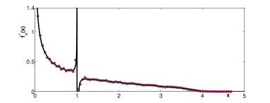
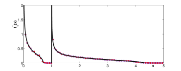
Figure 1: Equilibrium density of the Coulomb fluid, Eq. (15) for $\zeta=1$ (black solid line). The density in general has a disconnected support and exists in two different phases, depending on whether $\kappa$ is smaller (top panel) or larger (bottom panel) than $\kappa^{\star}(\zeta)$. Red dots correspond to Montecarlo simulations of a Coulomb gas of $20$ charges, where $7$ charges (top) and $12$ charges (bottom) were constrained to the right of $\zeta=1$ [26]. The corresponding values of the edge point $a$ are $a=1.04815>\zeta$ (top) and $a=0.701721<\zeta$ (bottom). The area under the leftmost blob is $1-\kappa$ and under the rightmost blob is $\kappa$.

We start by recalling some well known spectral properties of Wishart matrices (also known as Laguerre or chiral ensemble) defined earlier. The $N$ non-negative eigenvalues $\{\lambda_{i}\}$’of the Wishart matrix ${\mathbf{W}}$ are distributed via the joint probability density law [19]

$$\mathcal{P}(\lambda_{1},\ldots,\lambda_{N})=\frac{1}{Z_{N}}e^{-\frac{\beta}{2}\sum_{i=1}^{N}\lambda_{i}}\prod_{i=1}^{N}\lambda_{i}^{\frac{\beta}{2}\alpha}|\Delta(\mbox{\boldmath$\lambda$})|^{\beta}$$ (5)

where $\Delta(\mbox{\boldmath$\lambda$})=\prod_{j<k}(\lambda_{j}-\lambda_{k})$, $\alpha=(1+M-N)-2/\beta$ and $Z_{N}$ is the normalization constant. It is also known that for large $N$, $Z_{N}\simeq\exp[-\beta\Omega_{0}N^{2}]$ where $\Omega_{0}=3/4$ [20, 21]. This joint law (5) can be conveniently recast in the Boltzmann form

$$\mathcal{P}(\lambda_{1},\ldots,\lambda_{N})\propto\exp(-(\beta/2)E[\{\mbox{\boldmath$\lambda$}\}])$$ (6)

where the energy of a configuration $\{\mbox{\boldmath$\lambda$}\}$ is

$$E[\{\mbox{\boldmath$\lambda$}\}]=\sum_{i=1}^{N}\lambda_{i}-\alpha\sum_{i=1}^{N}\ln\lambda_{i}-\sum_{j\neq k}\ln|\lambda_{j}-\lambda_{k}|$$ (7)

Here, $\beta/2$ stands for the inverse temperature and for simplicity we focus here on almost-square matrices with $M-N$ (and thus $\alpha$) of $\mathcal{O}(1)$ for large $N$. This thermodynamical analogy, originally due to Dyson [22], allows to treat the system of eigenvalues as a Coulomb gas, i.e., a fluid of charged particles confined to the positive half-line by two competing interactions: the external linear + logarithmic potential (the first two terms) in (7) tends to push the charges towards the origin, while the third term representing mutual logarithmic repulsion between any pair of charges tends to spread them apart. It is useful first to estimate the typical scale of an eigenvalue $\lambda$ for large $N$. The first two terms typically scale for large $N$ as $\lambda_{\rm typ}N$ and $\ln(\lambda_{\rm typ})\,N$. In contrast, the pairwise Coulomb repulsion (the third term) typically scales as $N^{2}$ for large $N$. Balancing the first and the third term indicates $\lambda_{\rm typ}\sim N$ for large $N$. Consequently, as long as $\alpha\sim\mathcal{O}(1)$, the second term becomes smaller ($\sim\mathcal{O}(N)$) compared to the other two terms ($\sim\mathcal{O}(N^{2})$) and hence can be neglected. One then expects the average spectral density (normalized to unity) $\rho(\lambda)={N^{-1}}\sum_{i}\langle\delta(\lambda-\lambda_{i})\rangle$ to have the scaling form for large $N$: $\rho(\lambda)=N^{-1}\,f_{\mathrm{mp}}(\lambda/N)$. The scaling function $f_{\mathrm{mp}}(x)=(2\pi)^{-1}\sqrt{(4-x)/x}$ is the celebrated Marčenko-Pastur (MP) distribution on the compact support $x\in(0,4)$ [23].

Given the joint distribution in (5), our goal is to compute the statistics of $N_{+}$ denoting the number of eigenvalues greater than a fixed threshold value $\zeta N$, i.e., $N_{+}=\sum_{i=1}^{N}\theta(\lambda_{i}-\zeta N)$ where $\theta(x)$ is the Heaviside step function. The average value of $N_{+}$ can be easily estimated from the MP spectral density, $\langle N_{+}\rangle=N\,\int_{\zeta}^{4}f_{\mathrm{mp}}(x)dx=\kappa^{\star}(\zeta)N$ where $\kappa^{*}(\zeta)=(4\ \mathrm{arcsec}(2/\sqrt{\zeta})-\sqrt{\zeta(4-\zeta)})/2\pi$. The full probability distribution of $N_{+}$ can be written as the $N$-fold integral

$$\mathcal{P}(N_{+},N)\propto\int\prod_{i=1}^{N}d\lambda_{i}e^{-\beta E[\{\mbox{\boldmath$\lambda$}\}]}\delta\left(N_{+}-\sum_{i=1}^{N}\theta(\lambda_{i}-\zeta N)\right)$$ (8)

which we evaluate next for large $N$ by extending the Coulomb gas analogy mentioned above.

The evaluation of the $N$-fold integral (8) in the large $N$ limit consists of the following steps: first, we introduce an integral representation for the $\delta$ function, $\delta(x)=(2\pi)^{-1}(\beta N/2)\int dp\exp(\mathrm{i}\beta Npx/2)$. Then, we cast again the integrand in the Boltzmann form $\exp\left[-(\beta/2)E_{\kappa}(\{\mbox{\boldmath$\lambda$}\})\right]$ with $E_{\kappa}(\{\mbox{\boldmath$\lambda$}\})=E(\{\mbox{\boldmath$\lambda$}\})+A_{1}N\left(\sum_{i}\theta(\lambda_{i}-\zeta N)-\kappa N\right)$, where $A_{1}=\mathrm{i}p$ can be interpreted as a Lagrange multiplier. Written in this form, the integral has again a natural thermodynamical interpretation as the canonical partition function of a Coulomb gas in equilibrium at inverse temperature $\beta/2$. This time, however, in addition to the linear confinement and the logarithmic repulsion, the fluid particles (eigenvalues) are subjected to another (discontinuous) external potential. This external term involving $A_{1}$ in the new energy function $E_{\kappa}(\{\mbox{\boldmath$\lambda$}\})$ has the effect of constraining a fraction $\kappa$ of the fluid charges to the right of the point $x=\zeta N$.

In the large $N$ limit, the Coulomb gas with $N$ discrete charges becomes a continuous gas which can be described by a continuum (normalized to unity) density function $\varrho(\lambda)=N^{-1}\sum_{i=1}^{N}\delta(\lambda-\lambda_{i})$. Consequently, one can replace the original multidimensional integral in (8) by a functional integral over the space of $\varrho(\lambda)$. This procedure, originally introduced by Dyson [22], has recently been used successfully in a number of different contexts (see [24, 25, 21, 16, 17] and references therein). Noting further that the density $\varrho(\lambda)$ is expected to have the scaling form $\varrho(\lambda)=N^{-1}f_{\kappa}(\lambda/N)$ for large $N$, each term in the energy $E_{\kappa}(\{\mbox{\boldmath$\lambda$}\})$ is of the same order $\sim\mathcal{O}(N^{2})$ and is expressed as an integral over the function $f_{\kappa}(x)$ (see eq. (10) below). The scaled density $f_{\kappa}(x)$ satisfies the overall normalization condition $\int_{0}^{\infty}dxf_{\kappa}(x)=1$ and the constraint $\int_{0}^{\zeta}dxf_{\kappa}(x)=1-\kappa$ arising from the theta-function term in $E_{\kappa}(\{\mbox{\boldmath$\lambda$}\})$.

The probability (8) can now be rewritten as $\mathcal{P}(N_{+}=\kappa N,N)=Z_{\kappa}(N)/Z_{N}$, where the numerator $Z_{\kappa}(N)$ is the following functional integral over $f_{\kappa}(x)$, supplemented by two additional integrals over auxiliary variables $A_{1}$ and $A_{2}$ enforcing the two constraints mentioned above:

$$Z_{\kappa}(N)=\int dA_{1}\ dA_{2}\ \mathcal{D}[f_{\kappa}(x)]\exp\left\{-\frac{\beta}{2}N^{2}\mathcal{S}[f_{\kappa}(x)]\right\}.$$ (9)

The action $\mathcal{S}[f_{\kappa}(x)]$ is given by:

$$\mathcal{S}[f_{\kappa}(x)]=\int_{0}^{\infty}dxxf_{\kappa}(x)-\int_{0}^{\infty}\int_{0}^{\infty}dxdx^{\prime}f_{\kappa}(x)f_{\kappa}(x^{\prime})\ln|x-x^{\prime}|+A_{1}\left(\int_{0}^{\zeta}dxf_{\kappa}(x)-(1-\kappa)\right)+A_{2}\left(\int_{0}^{\infty}dxf_{\kappa}(x)-1\right)$$ (10)

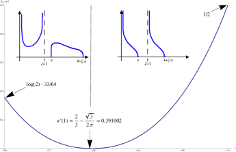
Figure 2: The rate function $\psi_{\zeta}$ as a function of $\kappa\in[0,1]$ from Eq. (18) for $\zeta=1$. In the two insets, a sketch of the corresponding Coulomb gas equilibrium densities (Eq. (15)) in the two regimes $\kappa<\kappa^{\star}(1)$ (left) and $\kappa>\kappa^{\star}(1)$ (right). Only at $\kappa=\kappa^{\star}(1)$ the two disconnected blobs of particles on both sides of the barrier at $\zeta=1$ merge into a single continuous density (the usual Marčenko-Pastur distribution $f_{\mathrm{mp}}(x)$).

Eq. (9) is indeed amenable to a saddle point analysis:

$$Z_{\kappa}(N)\approx\exp\left(-\frac{\beta}{2}N^{2}\mathcal{S}[f_{\kappa}^{\star}(x)]\right),\quad Z_{N}\approx\exp(-\beta\Omega_{0}N^{2})$$ (11)

where $\Omega_{0}=3/4$ and $f_{\kappa}^{\star}(x)$ is obtained from $\frac{\delta\mathcal{S}[f_{\kappa}(x)]}{\delta f_{\kappa}}=0$. This gives

$$x+A_{1}\theta(\zeta-x)+A_{2}=2\int dx^{\prime}f_{\kappa}^{\star}(x^{\prime})\log|x-x^{\prime}|$$ (12)

for all $x\in\mathsf{supp}(f_{\kappa}^{\star}(x))$ where $\mathsf{supp}$ denotes the region when charges exist, i.e., $f_{\kappa}^{\star}(x)$ is positive. Varying the action with respect to $A_{1}$ and $A_{2}$ just reproduces the two constraints. The function $f_{\kappa}^{\star}(x)$ obtained in this way is the rescaled equilibrium density of a Coulomb fluid where a fraction $\kappa$ of particles are constrained to lie to the right of a barrier at $x=\zeta$. It is easy to show [26] that $f_{\kappa}^{\star}(x)$ reduces to the unconstrained MP density $f_{\mathrm{mp}}(x)$ when $\kappa=\kappa^{\star}(\zeta)$.

Thus, for large $N$, the saddle point analysis precisely predicts the result in (2) with the rate function given by

$$\psi_{\zeta}(\kappa)=\frac{1}{2}\mathcal{S}[f_{\kappa}^{\star}(x)]-\Omega_{0}\,.$$ (13)

It then remains to solve the saddle-point equation (12). Taking one more derivative with respect to $x$ ($x\neq 0$):

$$\frac{1}{2}=\mathrm{Pr}\int\frac{f_{\kappa}^{\star}(x^{\prime})}{x-x^{\prime}}dx^{\prime}$$ (14)

where $\mathrm{Pr}$ denotes Cauchy’s principal value, supplemented with the constraints $\int_{0}^{\infty}dxf_{\kappa}^{\star}(x)=1$ and $\int_{0}^{\zeta}dxf_{\kappa}^{\star}(x)=1-\kappa$.

To invert the singular integral equation (14) is a nontrivial challenge. One often needs to guess the solution and verify it a posteriori. To get a feeling how the solution may look like, we first did a Monte Carlo simulation of the Coulomb gas which brought out the following very interesting features. For $\kappa\neq\kappa^{\star}(\zeta),0$ and $1$, the equilibrium charge density $f_{\kappa}^{\star}(x)$ (i) generally consists of two disconnected supports: a blob of $(1-\kappa)N$ eigenvalues to the left of $\zeta$ separated from a second blob of $\kappa N$ eigenvalues to the right of $\zeta$ (see Fig. 1), and (ii) the actual shapes of the two blobs depend on whether $\kappa<\kappa^{\star}(\zeta)$ (top panel of Fig. 1) or $\kappa>\kappa^{\star}(\zeta)$ (bottom panel of Fig. 1), i.e. the fluid undergoes a phase transition as $\kappa$ is varied across the critical point $\kappa^{\star}(\zeta)$. When $\kappa\to\kappa^{\star}(\zeta)$, the two blobs merge into a single support solution which is precisely the MP spectral density $f_{\mathrm{mp}}(x)$.

Extracting this two-support solution for a generic $\kappa\neq\kappa^{\star}(\zeta),0,1$ from the singular integral equation (14) poses the main technical challenge that we have succeeded in solving. There exists a well known Riemann-Hilbert method [27] for solving such singular integral equations when the solution has a single support [28]. For two disjoint supports, this method [27] was recently generalized in a number of different problems [16, 17, 29, 30, 31]. Adapting this generalized method to our problem (for details see [26]), we find that the two-support solution of (14) satisfying the two constraints is given explicitly by the expression

$$f_{\kappa}^{\star}(x)=\frac{1}{2\pi}\sqrt{\frac{(x-a)(4+\zeta-a-x)}{x(x-\zeta)}}.$$ (15)

The edge point $a$, depending on $\kappa$, is to be determined as the unique solution of the constraint $\int_{0}^{\zeta}dxf_{\kappa}^{\star}(x)=1-\kappa$, which can be rewritten in terms of generalized hypergeometric functions [26]. We have $a>\zeta$ for $\kappa<\kappa^{\star}(\zeta)$, $a<\zeta$ for $\kappa>\kappa^{\star}(\zeta)$ and $a=\zeta$ for $\kappa=\kappa^{\star}(\zeta)$. The density $f_{\kappa}^{\star}(x)$ is supported on the union of two disconnected intervals for $\kappa\neq\kappa^{\star}(\zeta)$, $[0,\zeta]\cup[a,4+\zeta-a]$ (if $\kappa\leq\kappa^{\star}(\zeta)$) or $[0,a]\cup[\zeta,4+\zeta-a]$ (if $\kappa\geq\kappa^{\star}(\zeta)$) [see, e.g., the insets of Fig. 2]. For $\kappa=\kappa^{\star}(\zeta)$, the two intervals merge into a single one and $f_{\kappa}^{\star}(x)=f_{\mathrm{mp}}(x)$ as expected. In the extreme cases $\kappa=0,1$, the density has also a single support and its analytical form is known from earlier works [21]. The function $f_{\kappa}^{\star}(x)$ is plotted in Fig. 1 for a specific choice $\zeta=1$, together with the result of Montecarlo simulations of the Coulomb gas, showing excellent agreement.

Next we substitute this explicit solution $f_{\kappa}^{\star}(x)$ in (10) to evaluate the saddle-point action $\mathcal{S}[f_{\kappa}^{\star}(x)]$. For this, we need to compute the single and double integrals in (10). The double integral can be written in terms of a simple integral after multiplying (12) by $f_{\kappa}^{\star}(x)$ and integrating over $x$. This leads to:

$$\mathcal{S}[f_{\kappa}^{\star}(x)]=\frac{1}{2}\left[\mu_{1}(\zeta)-A_{1}(1-\kappa)-A_{2}\right]$$ (16)

where $\mu_{n}(\zeta)=\int_{0}^{\infty}x^{n}f_{\kappa}^{\star}(x)dx$ is the $n$-th moment of the density. The first moment can be explicitly computed as $\mu_{1}(\zeta)=1-a+\frac{a^{2}}{4}+\zeta-\frac{a\zeta}{4}$. It remains to fix the two Lagrange multipliers $A_{1}$ and $A_{2}$, assigning suitable $x$ values in Eq. (12). Skipping details [26], it turns out that $A_{1}$ and $A_{2}$ can be expressed in terms of a pair of functions:

$$F_{(\pm)}=\frac{1}{2}\pm\frac{1}{2}\sqrt{\frac{(a-x)(4+\zeta-a-x)}{x(x-\zeta)}}$$ (17)

defined for $x\notin\mathsf{supp}(f_{\kappa}^{\star}(x))$. It can be shown that these functions are essentially the moment generating functions of $f_{\kappa}^{\star}(x)$ [26].

Combining (16) and (13), the final expression for the rate function $\psi_{\zeta}(\kappa)$ reads:

$$\psi_{\zeta}(\kappa)=\begin{cases}\frac{1}{4}\left[\tilde{\mu}(\zeta)-(1-\kappa)\left(a-\zeta-2\int_{\zeta}^{a}F_{(+)}(x)dx\right)-2\ln(4+\zeta-a)+2\int_{4+\zeta-a}^{\infty}dx\left(F_{(-)}(x)-\frac{1}{x}\right)\right],&\kappa\leq\kappa^{\star}(\zeta)\\ \frac{1}{4}\left[\tilde{\mu}(\zeta)-(1-\kappa)\left(\zeta-a-2\int_{a}^{\zeta}F_{(-)}(x)dx\right)-2\ln(4+\zeta-a)+2\int_{4+\zeta-a}^{\infty}dx\left(F_{(-)}(x)-\frac{1}{x}\right)\right],&\kappa\geq\kappa^{\star}(\zeta)\end{cases}$$ (18)

where $\tilde{\mu}(\zeta)=2-2a+a^{2}/4+2\zeta-a\zeta/4$. The behavior of $\psi_{\zeta}(\kappa)$ around the minimum $\kappa=\kappa^{\star}(\zeta)$ in (3) is found after a lengthy but straightforward expansion [26].

In summary, using a Coulomb gas approach we computed analytically the likelihood $P(N_{+}|\mathbf{W})$ of retaining $N_{+}$ principal components if a completely random (pure noise) $N\times N$ prior ${\mathbf{W}}$ (Wishart random matrix) is assumed for the underlying data. This likelihood is an essential ingredient in Bayes’ formula (1), which in turn gives the probability that a certain number $N_{+}$ of significant eigenvalues is observed if the data represents pure noise. Thus the rate function computed in (18) serves indeed as a benchmark to gauge the significance of results obtained for empirical data. We also found an interesting phase transition in the associated Coloumb gas problem when two separated blobs of Coulomb charges merge onto a single one as a critical value $N_{+}/N=\kappa=\kappa^{\star}(\zeta)$ is approached. This phase transition is responsible for the appearance of a logarithmic singularity in the rate function close to its minimum, which in turn leads to a highly universal logarithmic growth of the variance of $N_{+}$ with $N$.

The present work can be developed in several directions: on one hand, it would be interesting to analyze the case $N\neq M$ and check if the universality found for $N\simeq M$ still persists. On the other hand, improved stopping criteria based on null random matrix results are very much called for. The Coloumb gas method developed here for null random matrices may indeed be useful in that direction.

S.N.M. acknowledges the support of ANR grant 2011-BS04-013-01 WALKMAT.

References

- [1] S. S. Wilks, Mathematical Statistics (John Wiley & Sons, New York, 1962).
- [2] K. Fukunaga, Introduction to Statistical Pattern Recognition (Elsevier, New York, 1990).
- [3] L. I. Smith, A tutorial on Principal Components Analysis (2002).
- [4] N. Holter et al., Proc. Natl. Acad. Sci. USA 97, 8409 (2000).
- [5] O. Alter et al., Proc. Natl. Acad. Sci. USA 97, 10101 (2000).
- [6] L.-L. Cavalli-Sforza, P. Menozzi, and A. Piazza, The History and Geography of Human Genes (Princeton Univ. Press, 1994).
- [7] J. Novembre and M. Stephens, Nature Genetics 40, 646 (2008).
- [8] J.-P. Bouchaud and M. Potters, Theory of Financial Risks (Cambridge University Press, Cambridge, 2001).
- [9] Z. Burda and J. Jurkiewicz, Physica A 344, 67 (2004); Z. Burda, J. Jurkiewicz, and B. Wacław, Acta Phys. Pol. B 36, 2641 (2005) and references therein.
- [10] R. W. Preisendorfer, Principal Component Analysis in Meteorology and Oceanography (Elsevier, New York, 1988).
- [11] D. A. Jackson, Ecology 74, 2204 (1993).
- [12] L. Guttman, Psychometrika 19, 149 (1954); N. Cliff, Psychological Bulletin 103, 276 (1988).
- [13] G. D. Grossman and D. M. Nickerson, Ecology 72, 341 (1991).
- [14] J. O. Berger, Statistical Decision Theory and Bayesian Analysis (Springer Series in Statistics, 2nd ed., Springer-Verlag, 1985).
- [15] J. Wishart, Biometrika 20, 32 (1928).
- [16] S. N. Majumdar, C. Nadal, A. Scardicchio, and P. Vivo, Phys. Rev. Lett. 103, 220603 (2009).
- [17] S. N. Majumdar, C. Nadal, A. Scardicchio, and P. Vivo, Phys. Rev. E 83, 041105 (2011).
- [18] The symbol stands for the precise logarithmic law .
- [19] A.T. James, Ann. Math. Statistics 35, 475 (1964).
- [20] M. L. Mehta, Random Matrices (Academic Press, Boston, 1991).
- [21] P. Vivo, S. N. Majumdar, and O. Bohigas, J. Phys. A: Math. Theor. 40, 4317 (2007).
- [22] F. J. Dyson, J. Math. Phys. 3, 140 (1962).
- [23] V. A. Marčenko and L. A. Pastur, Math. USSR-Sb 1, 457 (1967).
- [24] D. S. Dean and S. N. Majumdar, Phys. Rev. Lett. 97, 160201 (2006).
- [25] D. S. Dean and S. N. Majumdar, Phys. Rev. E 77, 41108 (2008).
- [26] See Supplementary Material.
- [27] E. Brezin, C. Itzykson, G. Parisi, and J. B. Zuber, Commun. Math. Phys. 59, 35 (1978).
- [28] F. G. Tricomi, Integral Equations (Pure Appl. Math V, Interscience, London, 1957).
- [29] P. Vivo, S. N. Majumdar, and O. Bohigas, Phys. Rev. Lett. 101, 216809 (2008).
- [30] P. Vivo, S. N. Majumdar, and O. Bohigas, Phys. Rev. B 81, 104202 (2010).
- [31] K. Damle, S. N. Majumdar, V. Tripathi, and P. Vivo, Phys. Rev. Lett. 107, 177206 (2011).