Logarithmic entropy–corrected holographic dark energy with non–minimal kinetic coupling

Abstract

In this paper, we have considered a cosmological model with the non–minimal kinetic coupling terms and investigated its cosmological implications with respect to the logarithmic entropy– corrected holographic dark energy (LECHDE). The correspondence between LECHDE in flat FRW cosmology and the phantom dark energy model with the aim to interpret the current universe acceleration is also examined.

I Introduction

The universe acceleration, shown by several astronomical observations, indicates the existence of a mysterious exotic matter called dark energy (DE) Riess . In the classical gravity, whereas the cosmological constant, $\Lambda$, is the most prominent candidate of DE with the equation of state (EoS) parameter equals -1 Weinberg , there are strong evidence for a dynamical DE equation of state. However, the problem of DE Setare , its energy density and EoS parameter is still an unsolved problem in classical gravity and may be in the context of quantum gravity we achieve a more inclusive insight to its properties Cohen .

While in the microscopic level, the Einstein’s theory of gravity still remains unclear, the authors in J.M ; J.D ; S.W ; T.J obtain the first law of thermodynamics for black holes. Later, Padmanabhan proposes a thermodynamic interpretation of gravity T.P1 ; T.P2 . Recently, explanation of gravity as entropic force is pointed out by Verlinde E.P in several models such as specific microscopic model of space-time J.M1 , construction of holography from black hole entropy F.C and quantum information theories J-W . In addition, a modified entropic force in the Debye model is presented in Ref. C-J . For other relevant works in entropic force, see Refs. J.M2 ; Yu-X ; Jao-L ; I.V.V ; Y.Ti ; yun S ; Ah sh . In particular, the holographic principle is discussed in details by several authors F.W.Sh ; R.G.C ; y.z.g ; S.W.Wei ; Y.L.G.P ; SJM . In T1W , it has been shown that the holographic dark energy can be derived from the entropic force. The correspondence between entropy–corrected holographic and Gauss–Bonnet dark energy models is discussed is SeJa . Here, we intend to investigate the correspondence between logarithmic entropy–corrected holographic and cosmological models with kinetic terms coupled non–minimally to the scalar field and to the curvature L. N. Granda1 ; L. N. Granda2 ; L. N. Granda3 as a source of dark energy L. N. Granda1 ; L. N. Granda2 ; L. N. Granda3 . The initial motivation to study such theories is related to low energy limit of several higher dimensional theories.

The paper is organized as follows:

In section II, we review the scalar-tensor theories with non–minimally coupled kinetic terms to the curvature and the scalar field. We will obtain the field equations and energy–momentum tensors. In section III we introduce the basic setup of the ECHDE and obtain the corresponding EoS parameter for further investigation. In section IV, the correspondence between ECHDE and non-minimal kinetic coupling term and acceleration of the universe are presented. A short summary is given in section V.

II The model

The standard FRW cosmological is given by the metric,

$$ds^{2}=-dt^{2}+a(t)^{2}\left({dr^{2}\over 1-kr^{2}}+r^{2}(d\theta^{2}+\sin^{2}\theta d\phi^{2})\right),$$ (1)

where $a(t)$ is scale factor and $k=0,+1,-1$ imply the flat, close and open universe respectively. The energy-momentum tensor of a perfect fluid is given by $T^{\mu}_{\nu}=$ diag($-\rho,p,p,p)$. The Friedmann equations then are,

$$H^{2}=\frac{\kappa^{2}}{3}\rho,$$ (2)

$$\dot{H}=-\frac{\kappa^{2}}{2}(\rho+p).$$

We start with a cosmological model in which there is an interaction between a scalar field and the curvature L. N. Granda1 ; L. N. Granda2 ; L. N. Granda3

$$S= \int d^{4}x\sqrt{-g}\Big{[}\frac{1}{16\pi G}R-\frac{1}{2}\partial_{\mu}\phi\partial^{\mu}\phi-\frac{1}{2}\xi R\left(F(\phi)\partial_{\mu}\phi\partial^{\mu}\phi\right)-$$ (3)

$$\frac{1}{2}\eta R_{\mu\nu}\left(F(\phi)\partial^{\mu}\phi\partial^{\nu}\phi\right)-V(\phi)\Big{]},$$

where the coupling constants of dimensionless $\xi$ and $\eta$ are kinetic coupling and depend on the type of function $F(\phi)$.
Thus, by taking variation of action (3) with respect to the metric, we have,

$$R_{\mu\nu}-\frac{1}{2}g_{\mu\nu}R=\kappa^{2}\left[T_{\mu\nu}^{\phi}+T_{\mu\nu}^{\xi}+T_{\mu\nu}^{\eta}\right],$$ (4)

where $\kappa^{2}=8\pi G$.
The $T_{\mu\nu}^{\phi}$ is the energy-momentum tensor for the scalar field $\phi$, and $T_{\mu\nu}^{\xi}$ and $T_{\mu\nu}^{\eta}$ are the energy-momentum tensor for the minimally coupling $\xi$ and $\eta$ respectively. So, the corresponding energy-momentum tensors are,

$$T_{\mu\nu}^{\phi}=\nabla_{\mu}\phi\nabla_{\nu}\phi-\frac{1}{2}g_{\mu\nu}\nabla_{\lambda}\phi\nabla^{\lambda}\phi-g_{\mu\nu}V(\phi),$$ (5)

$$T_{\mu\nu}^{\xi}= \xi\Big{[}\left(R_{\mu\nu}-\frac{1}{2}g_{\mu\nu}R\right)\left(F(\phi)\nabla_{\lambda}\phi\nabla^{\lambda}\phi\right)+g_{\mu\nu}\nabla_{\lambda}\nabla^{\lambda}\left(F(\phi)\nabla_{\gamma}\phi\nabla^{\gamma}\phi\right)$$ (6)

$$-\frac{1}{2}(\nabla_{\mu}\nabla_{\nu}+\nabla_{\nu}\nabla_{\mu})\left(F(\phi)\nabla_{\lambda}\phi\nabla^{\lambda}\phi\right)+R\left(F(\phi)\nabla_{\mu}\phi\nabla_{\nu}\phi\right)\Big{]},$$

and

$$T_{\mu\nu}^{\eta}= \eta\Big{[}F(\phi)\left(R_{\mu\lambda}\nabla^{\lambda}\phi\nabla_{\nu}\phi+R_{\nu\lambda}\nabla^{\lambda}\phi\nabla_{\mu}\phi\right)-\frac{1}{2}g_{\mu\nu}R_{\lambda\gamma}\left(F(\phi)\nabla^{\lambda}\phi\nabla^{\gamma}\phi\right)$$ (7)

$$-\frac{1}{2}\left(\nabla_{\lambda}\nabla_{\mu}\left(F(\phi)\nabla^{\lambda}\phi\nabla_{\nu}\phi\right)+\nabla_{\lambda}\nabla_{\nu}\left(F(\phi)\nabla^{\lambda}\phi\nabla_{\mu}\phi\right)\right)$$

$$+\frac{1}{2}\nabla_{\lambda}\nabla^{\lambda}\left(F(\phi)\nabla_{\mu}\phi\nabla_{\nu}\phi\right)+\frac{1}{2}g_{\mu\nu}\nabla_{\lambda}\nabla_{\gamma}\left(F(\phi)\nabla^{\lambda}\phi\nabla^{\gamma}\phi\right)\Big{]}$$

In order to obtain the equation of motion for the scalar field, we take variation of action with respect to $\phi$, so we have,

$$-\frac{1}{\sqrt{-g}}\partial_{\mu}\left[\sqrt{-g}\left(\xi RF(\phi)\partial^{\mu}\phi+\eta R^{\mu\nu}F(\phi)\partial_{\nu}\phi+\partial^{\mu}\phi\right)\right]+\frac{dV}{d\phi}+$$ (8)

$$\frac{dF}{d\phi}\left(\xi R\partial_{\mu}\phi\partial^{\mu}\phi+\eta R_{\mu\nu}\partial^{\mu}\phi\partial^{\nu}\phi\right)=0.$$

For simplicity we assume that $\eta+2\xi$ = 0. Therefore, from Eqs. (5)-(8), the energy density, pressure and the scalar field equation are given by,

$$\rho=\frac{1}{2}\dot{\phi}^{2}+V(\phi)+9\xi H^{2}F(\phi)\dot{\phi}^{2},$$ (9)

$$p=\frac{1}{2}\dot{\phi}^{2}-V(\phi)-\xi\left(3H^{2}+2\dot{H}\right)F(\phi)\dot{\phi}^{2}-2\xi H\left(2F(\phi)\dot{\phi}\ddot{\phi}+\frac{dF}{d\phi}\dot{\phi}^{3}\right),$$ (10)

$$\ddot{\phi}+3H\dot{\phi}+\frac{dV}{d\phi}+3\xi H^{2}\left(2F(\phi)\ddot{\phi}+\frac{dF}{d\phi}\dot{\phi}^{2}\right)+18\xi H^{3}F(\phi)\dot{\phi}+12\xi H\dot{H}F(\phi)\dot{\phi}=0.$$ (11)

III Logarithmic entropy–corrected holographic dark energy

The black hole entropy plays a central role in the derivation of holographic dark energy (HDE). Indeed, the definition and derivation of holographic energy density depends on the entropy-area relationship $S\sim A\sim L^{2}$ of black holes in Einstein’s gravity, where $A\sim L^{2}$ represents the area of the horizon. However, this definition can be modified from the inclusion of quantum effects, motivated from the loop quantum gravity (LQG). The quantum corrections provided to the entropy-area relationship leads to the curvature correction in the Einstein-Hilbert action and vice versa 13 . The corrected entropy takes the form 14

$$S=\frac{A}{4}+\tilde{\gamma}\ln\Big{(}\frac{A}{4}\Big{)}+\tilde{\beta},$$ (12)

where $\tilde{\gamma}$ and $\tilde{\beta}$ are dimensionless constants of order unity. The exact values of these constants are not yet determined and are still debatable in LQC. The corrections are due to thermal equilibrium and quantum fluctuations 15 . The second term in (12) appears in a model of entropic cosmology which unifies the inflation and late time acceleration cai . The $\tilde{\gamma}$ might be extremely large due to current cosmological constraint, which inevitably brought a fine tuning problem to entropy corrected models and it is desirable to determine it by observational constrain. Taking the corrected entropy-area relation (12) into account, the energy density of the HDE will be modified as well. On this basis, Wei 16 proposed the energy density of the so-called ECHDE in the form

$$\rho_{\Lambda}=3c^{2}R_{h}^{-2}+\gamma R_{h}^{-4}\ln(R_{h}^{2})+\beta R_{h}^{-4},$$ (13)

in units where $M_{p}^{2}=8\pi G=1$, and $c$ is a constant determined by observational fit. The future event horizon $R_{h}$ is defined as,

$$R_{h}=a\int_{t}^{\infty}\frac{dt}{a}=a\int_{a}^{\infty}\frac{da}{Ha^{2}},$$ (14)

which leads to results compatible with observations. Furthermore, we can define the dimensionless dark energy as:

$$\Omega_{\Lambda}\equiv\frac{\rho_{\Lambda}}{3H^{2}}=\frac{3c^{2}+\gamma R_{h}^{-2}\ln(R_{h}^{2})+\beta R_{h}^{-2}}{3H^{2}R_{h}^{2}}.$$ (15)

In the case of a dark-energy dominated universe, dark energy evolves according to the conservation law,

$$\dot{\rho}_{\Lambda}+3H(\rho_{\Lambda}+p_{\Lambda})=0,$$ (16)

or equivalently

$$\dot{\Omega}_{\Lambda}=-\frac{2\dot{H}}{3H^{3}R_{h}^{2}}\left(3c^{2}+\gamma R_{h}^{-2}\ln(R_{h}^{2})+\beta R_{h}^{-2}\right)+\frac{HR_{h}-1}{3H^{2}R_{h}^{3}}\Big{[}-6c^{2}+2\gamma R_{h}^{-2}-4\gamma R_{h}^{-2}\ln R_{h}^{2}-4\beta R_{h}^{-3}\Big{]},$$ (17)

therefore the EoS parameter reduce to,

$$w_{\Lambda}=\frac{p_{\Lambda}}{\rho_{\Lambda}}=-1-\frac{2\gamma R_{h}^{-2}-4\gamma R_{h}^{-2}\ln(R_{h}^{2})-4\beta R_{h}^{-2}-6c^{2}}{3(3c^{2}+\gamma R_{h}^{-2}\ln(R_{h}^{2})+\beta R_{h}^{-2})}\left[1-\sqrt{\frac{3\Omega_{\Lambda}}{3c^{2}+\gamma R_{h}^{-2}\ln(R_{h}^{2})+\beta R_{h}^{-2}}}\right].$$ (18)

IV Correspondence between ECHDE and Non–minimal Kinetic coupling

Here we obtain the conditions for correspondence between our cosmological model with the non–minimal kinetic term and the ECHDE scenario in the flat FRW space. This can be achieved by obtaining an appropriate potential in the model. In the following we make two assumptions L. N. Granda2 ,
1) the function $F(\phi)$ is in exponential form as,

$$F(\phi)=\frac{1}{\phi_{0}^{2}}e^{2\lambda\phi},$$ (19)

and
2) the scalar factor is in power laws as $a=a_{0}t^{n}$, NOS . For negative $n$, the scale factor does not correspond to expanding universe but to shrinking one. If one changes the direction of time as $t\rightarrow-t$, the expanding universe whose scale factor is given by $a=a_{0}(-t)^{n}$ emerges. We note that when $t$ arrives $t_{s}$ occurs a big rip singularity, so this is an important scenario in relation with other cosmological singularities jims ; cai2 . Since $n$ is not an integer in general, the sign of $t$ is still a problem. To avoid the inconsistency, we may further shift the origin of the time as $-t\rightarrow t_{s}-t$. Then the time $t$ can be positive as long as $t<t_{s}$, and we can consistently take $a=a_{0}(t_{s}-t)^{n}$. So that, we can finally write scalar field as Ref. L. N. Granda2 in the following form,

$$H=\frac{n}{t},\hskip 28.45274pt\phi=\frac{1}{\lambda}\ln(\frac{\lambda\phi_{o}t}{\kappa\sqrt{\xi(1+3n)}}),$$ (20)

when $n>0$ or

$$H=\frac{-n}{t_{s}-t},\hskip 28.45274pt\phi=\frac{1}{\lambda}\ln\frac{\lambda\phi_{0}(t_{s}-t)}{\kappa\sqrt{\xi(1+3n)}},$$ (21)

when $n<0$. Here we first consider $n>0$ . If we establish a correspondence between the holographic dark energy and non–minimal coupling approach, then by using dark energy density equation (9) and relation (15), together with expressions (20), we easily arrive to the scalar potential as,

$$V=\frac{3n^{2}\lambda^{2}\phi_{0}^{2}}{\kappa^{4}\xi(1+3n)}\left(\kappa^{2}\Omega_{\Lambda}-\frac{3}{1+3n}\right)e^{-2\lambda\phi}$$ (22)

The equations (20) help us to obtain $t$ in terms of the scalar field $\phi$. Therefor, by substituting (19), (20), and (22) into (11), finally we have following equation,

$$3n-6n^{2}\lambda^{2}\Omega_{\Lambda}+\frac{18n^{2}\lambda^{2}}{\kappa^{2}(1+3n)}+3n^{2}\lambda\Omega_{\Lambda}^{\prime}+\frac{6n^{2}\lambda^{2}}{\kappa^{2}(1+3n)}\Big{(}3n\phi_{0}^{2}+1-3\phi_{0}^{2}\Big{)}e^{\frac{2\lambda\phi}{\phi_{0}^{2}}}e^{-2\lambda\phi}-1=0$$ (23)

where

$$\Omega_{\Lambda}^{\prime}=\frac{d\Omega_{\Lambda}}{d\phi}=\frac{d\Omega_{\Lambda}}{dt}\lambda t=\frac{d\Omega_{\Lambda}}{dt}\frac{\kappa\sqrt{\xi(1+3n)}}{\phi_{0}}\,e^{\lambda\phi}.$$ (24)

In order to have finite $R_{h}$, we consider the ansatz $a=a_{0}t^{n}$ for $n>1$ and substitute into equation (14), we then find:

$$R_{h}=\frac{t}{n-1},$$ (25)

$$\Omega_{\Lambda}=\frac{(n-1)^{2}}{3n^{2}}\Big{[}3c^{2}+\gamma\sigma^{-2}e^{-2\lambda\phi}\ln\{\sigma^{2}e^{2\lambda\phi}\}+\beta\sigma^{-2}e^{-2\lambda\phi}\Big{]},$$ (26)

and

$$w_{\Lambda}=-1-\frac{2\gamma\sigma^{-2}e^{-2\lambda\phi}-4\gamma\sigma^{-2}e^{-2\lambda\phi}\ln(\sigma^{2}e^{2\lambda\phi})-4\beta\sigma^{-2}e^{-2\lambda\phi}-6c^{2}}{3(3c^{2}+\gamma\sigma^{-2}e^{-2\lambda\phi}\ln(\sigma^{2}e^{2\lambda\phi})+\beta\sigma^{-2}e^{-2\lambda\phi})}$$

$$\times\left[1-\sqrt{\frac{3\Omega_{\Lambda}}{3c^{2}+\gamma\sigma^{-2}e^{-2\lambda\phi}\ln(\sigma^{2}e^{2\lambda\phi})+\beta\sigma^{-2}e^{-2\lambda\phi}}}\right].$$ (27)

where $\sigma=\frac{\kappa\sqrt{\xi(1+3n)}}{\lambda\phi_{0}(n-1)}$.
For $n<0$, we repeat the process, but impose relations (21). So, we find that,

$$V=\frac{3n^{2}\lambda^{2}\phi_{0}^{2}}{\kappa^{4}\xi(1+3n)}\left(\kappa^{2}\Omega_{\Lambda}-\frac{3}{1+3n}\right)e^{-2\lambda\phi}$$ (28)

and

$$3n-6n^{2}\lambda^{2}\Omega_{\Lambda}+\frac{18n^{2}\lambda^{2}}{\kappa^{2}(1+3n)}+3n^{2}\lambda\Omega_{\Lambda}^{\prime}+\frac{6n^{2}\lambda^{2}}{\kappa^{2}(1+3n)}\Big{(}3n\phi_{0}^{2}+1-3\phi_{0}^{2}\Big{)}e^{\frac{2\lambda\phi}{\phi_{0}^{2}}}e^{-2\lambda\phi}-1=0,$$ (29)

where

$$\frac{d\Omega_{\Lambda}}{d\phi}=-\frac{d\Omega_{\Lambda}}{dt}\lambda(t_{s}-t)=-\frac{d\Omega_{\Lambda}}{dt}\frac{\kappa\sqrt{\xi(1+3n)}}{\phi_{0}}\,e^{\lambda\phi}.$$ (30)

Now, under the ansatz $a=a_{0}(t_{s}-t)^{n}$ we can see from (14) that $R_{h}$ is always finite if $n<0$, which is just the case under investigation. Then we have:

$$R_{h}=\frac{t_{s}-t}{1-n},$$ (31)

$$\Omega_{\Lambda}=\frac{(n-1)^{2}}{3n^{2}}\Big{[}3c^{2}+\gamma\sigma^{-2}e^{-2\lambda\phi}\ln\{\sigma^{2}e^{2\lambda\phi}\}+\beta\sigma^{-2}e^{-2\lambda\phi}\Big{]},$$ (32)

and

$$w_{\Lambda}=-1-\frac{2\gamma\sigma^{-2}e^{-2\lambda\phi}-4\gamma\sigma^{-2}e^{-2\lambda\phi}\ln(\sigma^{2}e^{2\lambda\phi})-4\beta\sigma^{-2}e^{-2\lambda\phi}-6c^{2}}{3(3c^{2}+\gamma\sigma^{-2}e^{-2\lambda\phi}\ln(\sigma^{2}e^{2\lambda\phi})+\beta\sigma^{-2}e^{-2\lambda\phi})}$$

$$\times\left[1-\sqrt{\frac{3\Omega_{\Lambda}}{3c^{2}+\gamma\sigma^{-2}e^{-2\lambda\phi}\ln(\sigma^{2}e^{2\lambda\phi})+\beta\sigma^{-2}e^{-2\lambda\phi}}}\right].$$ (33)

The phantom crossing then occurs for the EoS parameter of the ECHDE model in the following scenario rev :

$$2\gamma\sigma^{-2}e^{-2\lambda\phi}-4\gamma\sigma^{-2}e^{-2\lambda\phi}\ln(\sigma^{2}e^{2\lambda\phi})-4\beta\sigma^{-2}e^{-2\lambda\phi}-6c^{2}>0,$$ (34)

$$3\Omega_{\Lambda}<3c^{2}+\gamma\sigma^{-2}e^{-2\lambda\phi}\ln(\sigma^{2}e^{2\lambda\phi})+\beta\sigma^{-2}e^{-2\lambda\phi}.$$ (35)

and

$$2\gamma\sigma^{-2}e^{-2\lambda\phi}-4\gamma\sigma^{-2}e^{-2\lambda\phi}\ln(\sigma^{2}e^{2\lambda\phi})-4\beta\sigma^{-2}e^{-2\lambda\phi}-6c^{2}<0,$$ (36)

$$3\Omega_{\Lambda}>3c^{2}+\gamma\sigma^{-2}e^{-2\lambda\phi}\ln(\sigma^{2}e^{2\lambda\phi})+\beta\sigma^{-2}e^{-2\lambda\phi}.$$ (37)

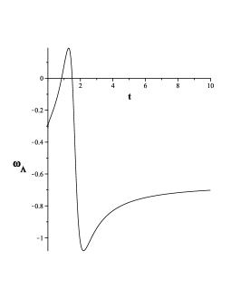
Figure 1: Graph of the EoS parameter $(n>0)$ in terms of time evolution by choosing $c=0.5$, $\gamma=-2$, $n=2$ and $\beta=0.25$.

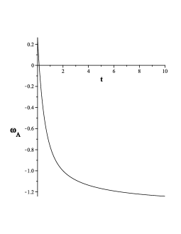
Figure 2: Graph of the EoS parameter $(n<0)$ in terms of time evolution by choosing $c=3$, $\gamma=-2$, $n=-2$, $t_{s}=-1$ and $\beta=2$.

Using numerical calculation, the EoS parameter for both positive and negative $n$ are given in the Figs. 1 and 2. Also we can see in both cases with different EoS parameters which the phantom crossing occurs.

V Conclusion

In this paper we started with scalar tensor theories with the non–minimal kinetic coupling to gravity and obtained the corresponding field equations, energy density and pressure. We introduced the logarithmic entropy–corrected holographic energy density as a dynamical cosmological constant. In order to obtain the cosmological parameters, we need to explicitly define the function $F(\phi)$. The popular exponential form is chosen with the motivation to produce phantom crossing behavior in formalism.
We obtained different conditions in order to have a correspondence between entropy–corrected holographic and non-minimal kinetic coupling dark energy model. Also we reconstructed potential in terms of field $\phi$ for two cases $n>0$ and $n<0$. Finally we obtained the EoS parameter for the holographic energy density in the model with the condition for phantom crossing scenario given by (34)-(37).

VI Acknowledgements

The authors are indebted to the anonymous referee for his/her comments that improved the Letter drastically.

References

• (1) A. G. Riess et al., Astron. J. 116, 1009 (1998); S. Perlmutter et al., As23 trophys. J. 517, 565, (1999).
• (2) S. Weinberg, Rev. Mod. Phys. 61, 1, (1989). V. Sahni and A. A. Starobinsky, Int. J. Mod. Phys. D 9, 373, (2000).
• (3) M. R. Setare, Phys. Lett. B 654, 1-6 (2007); M. R. Setare, Eur. Phys. J. C 50, 991-998 (2007); M. R. Setare, Phys. Lett. B 642, 421-425 (2006); M. R. Setare, Phys. Lett. B 648, 329-332 (2007); M. R. Setare, Phys. Lett. B 653, 116-121 (2007); M. U. Farooq, M. Jamil and U. Debnath, Astrophys. Space Sci. 334, 243-248 (2011).
• (4) A. G. Cohen, D. B. Kaplan and A. E. Nelson, Phys. Rev. Lett. 82, 4971, (1999).
• (5) J. M. Bardeen, B. Carter and S. W. Hawking, Commun. Math. Phys. 31, 161 (1973).
• (6) J. D. Bekenstein, Phys. Rev. D 7, 949 (1973). J. D. Bekenstein, Phys. Rev. D 7, 2333 (1973).
• (7) S. W. Hawking, Commun. Math. Phys. 43, 199 (1975).
• (8) T. Jacoson, Phys. Rev. Lett. 75, 1260 (1995).
• (9) T. Padmanabhan, Class. Quantum Grav. 21, 4485 (2004).
• (10) T. Padmanabhan,arXiv:0911.5004 [gr-qc].
• (11) E. P. Verlinde, arXiv:1001.0785 [hep-th].
• (12) J. Makela, arXiv:1001.3808 [gr-qc].
• (13) F. Caravelli and L. Monesto, arXiv:1001.4364 [gr-qc].
• (14) J.-W. Lee, H.-C. Kim and J. Lee , arXiv:1001.5445 [hep-th].
• (15) C.-J. Cao, Phys. Rev. D 81 087306 (2010).
• (16) Joakim Munkhammar, arXiv:1003.1262 [hep-th]
• (17) Yu- Xiao Liu, Yong-qiang Wang and Shao -Wen Wei, arXiv:1002.1062 [hep-th]. L. Zhao, arXiv:1002.0488 [hep-th]. Zhaoyue, arXiv:1002.4039 [hep-th]. Xiao-Gang He and Bo-Qiang Ma, Chin. Phys. Lett. 27 070402 (2010). Xin Li and Zhe chang, arXiv:1005.1169[hep-th]. Hao Wei, arXiv:1005.1445 [gr-qc]. Bin Liu, Yun-Chuan Dai, Xian- Ru Hu, Jian - Bo Deng, arXiv:1007.2987 [hep-th]. Bin Liu, Yun-Chuan Dai, Xian- Ru Hu, Jian - Bo Deng, arXiv:1007.2985 [hep-th].
• (18) Jao-Weon Lee, arXiv:1003.4464 [hep-th]. Ee Chang-Young, Myungseok Eune and Kyoungtae Kimm, arXiv:1003.2049[gr-qc]. Yun Soo Myung and Yong - Wan Kim, arXiv:1002.2292 [hep-th].
• (19) I. V. Vancea and M. A. Santos, arXiv:1002.2454 [hep-th]. Jerzy Kowalski-Glikman, arXiv:1002.1035 [hep-th]. R. A. Konoplya, arXiv:1002.2818 [hep-th]. Sauav Samanta, arXiv:1003.5965 [hep-th].
• (20) Y. Tian and X. N. Wu, Phys. Rev. D 81 104013 (2010).
• (21) Yun soo myung, Phys. Rev. D 81 105012 (2010).
• (22) A. Sheykhi, Phy. Rev. D 81 104011 (2010); M. Jamil and A. Sheykhi, Int. J. Theor. Phys. 50, 625-636 (2011).
• (23) F.-W. Shu and Y.-G. Gong, arXiv:1001.3237 [gr-qc].
• (24) R.-G. Cai, L.-M. Cao and N. Ohta, Phys. Rev. D 81 061501 (R) (2010).
• (25) Y. Zhang, Y.-G. Gong and Z.-H. Zhu, arXiv:1001.4677 [hep-th].
• (26) S.-W. Wei, Y. -X. Liu and Y.-Q. Wang,arXiv:1001.5238 [hep-th].
• (27) Y. Ling and J.-P. Wu, arXiv:1001.5324 [hep-th].
• (28) A. Sheykhi, M. Jamil, arXiv:1011.0134v2 [physics.gen-ph].
• (29) M. Li and Y. Wang, Phys. Lett. B 687 243 (2010).
• (30) M. R. setare and Mubasher Jamil, Europhys. Lett. 92 49003 (2010).
• (31) L. N. Granda, arXiv:0911.3702 [hep-th]
• (32) L. N. Granda, JCAP 07, 021 (2010); arXiv:1005.2716 [hep-th]
• (33) L. N. Granda, arXiv:1009.3964 [hep-th]
• (34) T. Zhu and J-R. Ren, Eur. Phys. J. C 62 (2009) 413;
R-G. Cai et al, Class. Quant. Grav. 26 (2009) 155018.
• (35) M. Jamil and M. U. Farooq, J. Cosmol. Astropart. Phys. 03 (2010) 001;
R. Banerjee and S. K. Modak, JHEP 0905 (2009) 063;
H.M. Sadjadi and M. Jamil, Gen. Rel. Grav. 43 1759-1775 (2011).
• (36) C. Rovelli, Phys. Rev. Lett. 77 (1996) 3288;
A. Ashtekar et al, Phys. Rev. Lett. 80 (1998) 904;
A. Ghosh and P. Mitra, Phys. Rev. D 71 (2005) 027502.
• (37) Y. F. Cai, J. Liu, H. Li, Phys. Lett. B 690, 213, (2010).
• (38) H. Wei, Commun. Theor. Phys. 52, 743 (2009).
• (39) S. Nojiri, S. D. Odintsov and M. Sasaki, Phys. Rev. D 71, 123509 (2005).
• (40) R. R. Caldwell, M. Kamionkowski, N. N. Weinberg Phys. Rev. Lett. 91 (2003) 071301.
• (41) Y. F. Cai, H. Li, Y. S. Piao, X. Zhang, Phys. Lett. B 646, 141, (2007);
Y. F. Cai, T. Qiu, R. Brandenberger, X. Zhang, Phys. Rev. D80, 023511, (2009).
• (42) E.J. Copeland, M. Sami and S. Tsujikawa, Int. J. Mod. Phys. D 15 (2006) 1753.