Creep motion of a model frictional system

Abstract

We report on the dynamics of a model frictional system submitted to minute external perturbations. The system consists of a chain of sliders connected through elastic springs that rest on an incline. By introducing cyclic expansions and contractions of the springs we observe a reptation of the chain. We account for the average reptation velocity theoretically. The velocity of small systems exhibits a series of plateaus as a function of the incline angle. Due to elastic effects, there exists a critical amplitude below which the reptation is expected to cease. However, rather than a full stop of the creep, we observe in numerical simulations a transition between a continuous-creep and an irregular-creep regime when the critical amplitude is approached. The latter transition is reminiscent of the transition between the continuous and the irregular compaction of granular matter submitted to periodic temperature changes.

I Introduction.

Granular materials are collections of macroscopic particles (grains) that interact via dissipative forces. As a result, external excitation is necessary to promote the motion of the grains. In general, it is assumed that in absence of mechanical perturbations, such materials will eventually reach a mechanically static configuration and remain at rest. In particular, thermal agitation will not suffice to induce rearrangements and, for this reason, granular matter is said to be athermal knight95 ; philippe02 ; pouliquen03 . This is however a simplified view that assumes an idealized situation in which all perturbation (temperature variations, humidity changes, mechanical noise, etc.), even minute, can be suppressed.

In practice, small temperature variations can actually trigger small but measurable rearrangements of the structure. Uncontrolled thermal dilations have been reported to generate stress fluctuations large enough to hinder reproducible measurements of the stress field inside a granular pile vanel99 ; clement97 . They were even suspected to be the driving factor leading to large-scale ’static avalanches’ claudin97 . When accumulating, such minute perturbations can induce an irreversible evolution of the system. Several recent studies indeed showed that temperature cycles, even of small amplitude, can induce the slow compaction (a creep) of dry granular materials geminard03 ; chen06 ; chen09 ; divoux08 ; divoux09 ; divoux09t ; divoux10 . Moreover, a transition between a continuous-flow and an intermittent-flow regime, observed when the amplitude of the temperature cycles is decreased divoux08 ; divoux09 ; divoux09t ; divoux10 , remains unexplained. Even if the transition is thought to be due to finite size effects (i.e. the finite number of grains in the diameter of the tube), the mechanisms, in particular the role played by the confining walls, are still under debate.

In the same manner, minute temperature changes have been identified, more than a century ago, to induce the creep of solids in frictional contacts. H. Moseley reported first the descent, driven by temperature variations, of lead plates covering the south side of the choir of Bristol cathedral and mentionned that the same mechanism could be responsible for the motion of glaciers moseley . A macroscopic model, considering only the relative dilations of the solids in contact, predicts that the creep velocity is proportional to the amplitude of the temperature changes moseley ; bouasse and, thus, that any temperature variation, whatever its amplitude, leads to a motion. However, as noticed by H. Bouasse, such a description does not take into account the elastic effects which necessarily play a role for large systems bouasse . When elastic effects come into play, the temperature variations are sufficient to induce the motion only if their amplitude is larger than a critical value which, in particular, increases with the size of the system croll09 . Accordingly, for a given amplitude of the temperature variations, a solid is observed to descent along an incline only if the tilt angle is large enough tamburi74 .

In the present article, we propose the study of a model mimicking the reptation along an incline of a solid subjected to temperature variations. We remark that the aforementioned models disregard the fact that the surfaces, even if nominally flat, are in real contact in a finite number of localized regions. However, due to roughness, the real contact between the surfaces reduces to a large, but finite, number of microcontacts, themselves belonging to a small number of mesoscopic, coherent, contact regions persson10 . Such coherent regions are composed of a large number of microcontacts, so that their contact with the substrate obeys the Amonton-Coulomb law for static friction. We thus consider a set of sliders, connected by springs, in frictional contact with an incline and subjected to temperature changes. We report and discuss an extensive study of the associated dynamics. We point out that, interestingly, the conclusions help in understanding the observations reported for a granular material in a tube.

II The model

II.1 Description

The system (total mass $M$) consists of a series of $N$ identical sliders (zero length, mass $m=M/N$) connected by $(N-1)$ identical springs (massless, stiffness $k$). The sliders are in frictional contact with an incline which makes an angle, $\alpha$, with the horizontal (Fig. 1). They are subjected to the forces due to the springs, to their own weight $mg$ (where $g$ denotes the acceleration due to gravity) and to the reaction force from the incline (including the frictional force).

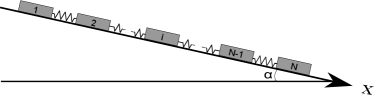
Figure 1: Sketch of the model system.

The aim of the study is to account for the dynamics of the system induced by temperature changes. To do so, we consider that the natural length of the springs, $l$, depends linearly on the temperature $T$ according to:

$$l(T)=l_{0}\bigl{[}1+\kappa(T-T_{0})\bigr{]}$$ (1)

where $\kappa$ stands for the thermal expansion coefficient of the slider material and $l_{0}$ for the natural length of the springs at $T_{0}$. In accordance, the total length of the system at $T_{0}$, in absence of internal stress, is $L=(N-1)\,l_{0}$. We further assume, for the sake of simplicity, that the stiffness $k$ does not depend on the temperature and that the substrate does not dilate.

From now on, the $x$-axis is oriented downwards, $\alpha$ is positive and the first slider is the upper one (Fig. 1). Thus, at the temperature $T$, the force due to the spring, exerted by the slider $(n+1)$ on the slider $n$ is:

$$f_{n+1\to n}=-k\,\left[x_{n}-x_{n+1}+l(T)\right]$$ (2)

where $x_{n}$ denotes the position of the slider $n$ on the incline.

At rest, the contact between the sliders and the incline is characterized by the static frictional coefficient $\mu_{\mathrm{s},n}$ such that the slider $n$, initially at rest, starts moving if:

$$\left|f_{n+1\to n}+f_{n-1\to n}+mg\,\sin\alpha\right|>\mu_{\mathrm{s},n}\,mg\,\cos\alpha.$$ (3)

We remark that, at the boundaries, $f_{0\to 1}=0$ ($n=1$) and $f_{N+1\to N}=0$ ($n=N$). Note that, due to the spatial heterogeneity of the incline surface, the static frictional coefficient might take, at random, different values, $\mu_{\mathrm{s},n}$, for the different sliders which lie at different positions, $x_{n}$, on the incline baumberger06 . In accordance, a slider that moves and stops at a different position might be then associated with a different value of $\mu_{\mathrm{s},n}$. By contrast, we assume that, when the slider is in motion, the frictional contact is characterized by a single, constant, dynamical frictional coefficient, $\mu_{\mathrm{d}}$. Indeed, while in motion, the slider explores the incline and is thus less sensitive to the details of the surface properties. The constant $\mu_{\mathrm{d}}$ quantifies the average rate of energy dissipation and the slider $n$ in motion is subjected to the associated dynamical frictional force:

$$f_{\mathrm{d},n}\equiv-\mu_{\mathrm{d}}\,mg\,\cos\alpha\,S(\dot{x}_{n})$$ (4)

where $\dot{x}_{n}$ denotes the velocity and $S$ the sign function [$S(u)=1$ if $u>0$ and $S(u)=-1$ if $u<0$]. We further assume, in agreement with standard observations, that $\mu_{\mathrm{d}}<\mu_{\mathrm{s},n}$ $(\forall n)$, i.e., the dynamical frictional coefficient is smaller than the static one.

The mechanical system is submitted to temperature changes. Some sliders, initially at rest, start moving when the length $l(T)$ exceeds a value such that the condition (3) is satisfied for, at least, one slider. Submitted to the forces due to the springs, to their own weight and to the reaction force from the incline (including the frictional force), one or more sliders move and come back to rest. Such event constitutes, by definition, a “mechanical rearrangement” of the system. At this point, it is interesting to consider two characteristic times. On the one hand, due to its thermal inertia, the system exhibits a thermal characteristic time $\tau_{\mathrm{th}}$ which limits the dynamics of the temperature changes and, thus, of the thermal dilations. In practice, for a macroscopic system whose typical size $L$ ranges from a few millimeters to centimeters, $\tau_{\mathrm{th}}$ ranges from seconds to hours. On the other hand, the dynamics of the mechanical system is characterized by the typical time scale $\tau_{\mathrm{dyn}}=\sqrt{m/k}$. In practice, one can consider instead that $\tau_{\mathrm{dyn}}\sim L/c_{\mathrm{s}}$ where $c_{\mathrm{s}}$ stands of the speed of sound in the material the macroscopic solid is made of. For a typical size $L$ ranging from a few millimeters to centimeters and usual values of $c_{\mathrm{s}}$ (about a few kilometers per second), we estimate $\tau_{\mathrm{dyn}}\sim 10^{-6}-10^{-5}$ s, thus much smaller than $\tau_{\mathrm{th}}$. As a consequence, we consider that $l(T)$ is constant during the mechanical rearrangements which are, in practice, much faster than the temperature variations.

II.2 General system of equations

II.2.1 Mechanical system

First, we write the differential equation governing the position $x_{\mathrm{n}}$ of the slider $n$, when the latter is in motion. Introducing the thermal dilation $\theta\equiv\kappa\,(T-T_{0})$ and the dimensionless variables $\tilde{t}\equiv t/\tau_{\mathrm{dyn}}$ and $\tilde{x}\equiv x/(g\,\tau_{\mathrm{dyn}}^{2})$ (with $\tau_{\mathrm{dyn}}\equiv\sqrt{m/k}$), we get:

$$\ddot{\tilde{x}}_{1} = -[\tilde{x}_{1}-\tilde{x}_{2}+(1+\theta)\,\tilde{l}_{0}]$$ (5)

$$-\mu_{\mathrm{d}}\,S(\dot{\tilde{x}}_{1})\,\cos{\alpha}+\sin\alpha~{}~{}~{}~{}~{}\left(n=1\right)$$

$$\ddot{\tilde{x}}_{n} = -[2\,\tilde{x}_{n}-(\tilde{x}_{n+1}+\tilde{x}_{n-1})]$$ (6)

$$-\mu_{\mathrm{d}}\,S(\dot{\tilde{x}}_{n})\,\cos{\alpha}+\sin\alpha~{}~{}~{}~{}~{}\left(n\neq 1,N\right)$$

$$\ddot{\tilde{x}}_{N} = -[\tilde{x}_{N}-\tilde{x}_{N-1}-(1+\theta)\,\tilde{l}_{0}]$$ (7)

$$-\mu_{\mathrm{d}}\,S(\dot{\tilde{x}}_{N})\,\cos{\alpha}+\sin\alpha~{}~{}~{}~{}~{}\left(n=N\right)$$

where, in accordance, we defined $\tilde{l}_{0}\equiv l_{0}/(g\,\tau_{\mathrm{dyn}}^{2})$.

Second, we remind that the slider $n$, if at rest, starts moving if the condition (3) is satisfied. Thus, using the dimensionless variables, we can write:

$$|\tilde{x}_{2}-\tilde{x}_{1}-(1+\theta)\,\tilde{l}_{0}+\sin\alpha| > \mu_{\mathrm{s},1}\,\cos\alpha$$ (8)

$$|\tilde{x}_{n+1}+\tilde{x}_{n-1}-2\,\tilde{x}_{n}+\sin\alpha| > \mu_{\mathrm{s},n}\,\cos\alpha$$ (9)

$$|\tilde{x}_{N-1}-\tilde{x}_{N}+(1+\theta)\,\tilde{l}_{0}+\sin\alpha| > \mu_{\mathrm{s},N}\,\cos\alpha$$ (10)

where the conditions (8) and (10) apply for the slider 1 and $N$ respectively and the condition (9) for any other slider $n\neq 1,N$.

II.2.2 Frictional contact

We remind that the dynamical frictional contact between the sliders and the incline is characterized by a single coefficient, $\mu_{\mathrm{d}}$. By contrast, each time a slider in motion comes back to rest, a new value of the static frictional coefficient $\mu_{\mathrm{s}}$ is drawn from a probability distribution $p(\mu_{\mathrm{s}})$. In order to evaluate if the fluctuations in $\mu_{\mathrm{s}}$ are relevant for explaining the qualitative behaviour of the system and to be able to discuss the results analytically, we assume that $p(\mu_{\mathrm{s}})$ is a Gaussian distribution, namely

$$p(\mu_{\mathrm{s}})=\frac{1}{\sqrt{2\pi\sigma_{\mu}^{2}}}\exp\left[-\frac{(\mu_{\mathrm{s}}-\overline{\mu}_{\mathrm{s}})^{2}}{2\sigma_{\mu}^{2}}\right]$$ (11)

where $\overline{\mu}_{\mathrm{s}}$ denotes the average value and $\sigma_{\mu}$ the width of the distribution. We point out that, the distribution $p(\mu_{\mathrm{s}})$ does not, strictly speaking, satisfy the condition $p(\mu_{\mathrm{s}})=0$, $\forall\mu_{\mathrm{s}}<\mu_{\mathrm{d}}$ (i.e., the static friction coefficient can be smaller than the dynamic one). However, we restrict our study to the case $\sigma_{\mu}\ll(\overline{\mu}_{\mathrm{s}}-\mu_{\mathrm{d}})$, so that the latter condition is reasonably satisfied in practice.

II.2.3 Temperature variations

The system is driven by temperature variations which induce changes in the natural length of the springs. We will either consider that the temperature oscillates with the period $2\tau_{\mathrm{th}}$ between two well-defined values such that the dilation oscillates periodically between $-A_{\theta}$ and $+A_{\theta}$, or that the temperature $T$ of the system fluctuates around the temperature $T_{0}$ with a typical amplitude $\Delta T$ such that $\theta$ fluctuates around zero with a typical amplitude $\sigma_{\theta}\sim\kappa\,\Delta T$. In this latter case, in order to be able to discuss the results analytically, we shall assume that, at a series of equally-spaced timesteps $t_{q}\equiv q\,\tau_{\mathrm{th}}$ ($q\in\mathbb{N}$), a value $\theta_{q}$ of the dilation is drawn from the Gaussian distribution:

$$\psi(\theta)=\frac{1}{\sqrt{2\pi\sigma_{\theta}^{2}}}\exp\left[-\frac{\theta^{2}}{2\sigma_{\theta}^{2}}\right]$$ (12)

where $\sigma_{\theta}$ accounts for the typical amplitude of the thermal dilations. We then assume that $\theta=\theta_{q}$ for $t\in[t_{q},t_{q+1}[$.

II.3 Numerical method

Consider that, when the time $t$ reaches $t_{q+1}$, the system already experienced $k$ mechanical rearrangements such that all the sliders are resting at the positions $\tilde{x}_{n}^{k}$ associated with the static frictional coefficients $\mu_{\mathrm{s},n}^{k}$ ($n\in[1,N]$). At $t=t_{q+1}$, a new value $\theta_{q+1}$ of $\theta$ is drawn at random according to the distribution $\psi(\theta)$. The subsequent evolution of the system is obtained as follows.

From the conditions (8)-(10), one calculates the first critical value $\theta_{c}^{k+1}$ which leads to the destabilization of at least one slider (in general, $|\theta_{c}^{k+1}|<|\theta_{q+1}|$). Then, for $\theta=\theta_{c}^{k+1}$, the equations (5)-(7) are integrated numerically using an integration time step $\Delta t\ll\tau_{\mathrm{dyn}}$ (we use a standard velocity Verlet integrator numerical_recipes ). In order to take into account that the motion of one slider can destabilize its neighbours, the procedure checks if any condition (8)-(10) for the sliders at rest is fulfilled within each timestep $\Delta t$. If so, the motion of the corresponding slider(s) is also accounted for through (5)-(7). In the same way, the procedure checks at each timestep if any of the sliders in motion comes to rest. If so, a new value of the associated static frictional coefficient is drawn at random according to the distribution $p(\mu_{\mathrm{s}})$ [Eq. (11)]. We consider that the mechanical rearrangement ends when all the sliders are back to rest. All the sliders are then resting at the new positions $\tilde{x}_{n}^{k+1}$, associated with a new set of static frictional coefficients $\mu_{\mathrm{s},n}^{k+1}$.

The procedure is iterated by finding, in the same way, the next critical value of the dilation $\theta_{c}$ which leads, according to the conditions (8)-(10), to the next mechanical rearrangement. For each $\theta_{c}$, a new static state of the system is found. The procedure stops when the next critical dilation $\theta_{c}$ is beyond $\theta_{q+1}$. The system then experienced $k^{\prime}$ rearrangements. The $\tilde{x}_{n}^{k^{\prime}}$ are then the positions of the sliders at $t=t_{q+2}$.

The long-term behavior of the system is assessed by iterating the whole procedure, either making $\theta$ oscillate between $-A_{\theta}$ and $+A_{\theta}$ or drawing at random the next value of $\theta$ according to the distribution $\psi(\theta)$.

III Results

III.1 The minimal system: 2 sliders

Consider first the system consisting of two sliders ($N=2$) connected by one spring. The system is very similar to that already studied in Ref. geminard10 for the case of a horizontal substrate but, now, the system lies on an incline which makes a finite angle $\alpha$ with the horizontal.

III.1.1 Numerical results

In order to account for the creep of the system along the slope we consider the position of the center of mass $\tilde{x}_{G}\equiv\frac{1}{N}\,\sum_{n=1}^{N}\tilde{x}_{n}$ (here $N=2$) as a function of time at the timesteps $t_{q}$ [Fig. (2)] for Gaussian variations of the temperature (Eq. 12). We observe that, for a sufficiently large $\sigma_{\theta}$, the center of mass moves downwards with, in average, the constant velocity $<\tilde{v}_{G}>$.

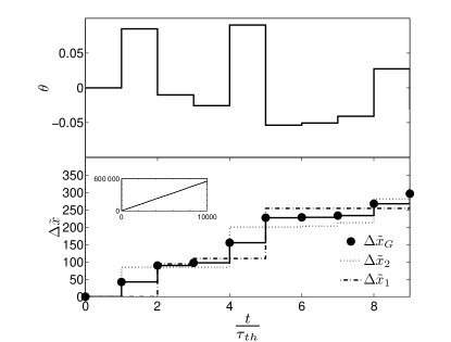
Figure 2: Creep motion of 2 sliders – Top: The dilation $\theta$ evolves randomly according to the Gaussian distribution (12). Bottom: In response to the dilations, the whole systems creeps along the incline. We report the displacements $\Delta\tilde{x}_{1}$ and $\Delta\tilde{x}_{2}$ of the sliders, as well as the displacement $\Delta\tilde{x}_{G}$ of the center of mass with respect to their initial positions. We observe that the lower slider moves in response to dilations whereas the upper slider moves in response to contractions. Note that both sliders move systematically downwards. Inset: Long-time behavior – $\Delta\tilde{x}_{G}$ increases linearly with time $t$, the system is creeping at constant velocity ($\tilde{l}_{0}=10^{3}$, $\mu_{\mathrm{d}}$=0.5, $\overline{\mu}_{\mathrm{s}}$=0.6, $\sigma_{\mu}$ = 0.01, $\sigma_{\theta}$ =0.1 and $\tan{\alpha}$ = 0.25).

For a given amplitude of the temperature variations $\sigma_{\theta}$, we observe that the average creep velocity of the center of mass, $<\tilde{v}_{G}>$, depends only slightly on the slope over a wide range of the angle $\alpha$ (Fig. 3). Indeed, for small $\alpha$, $<\tilde{v}_{G}>$, which equals zero for $\alpha=0$, increases rapidly with $\alpha$ and reaches a plateau for a typical value that we denote $\alpha_{\mathrm{c}}^{-}$. Then, above $\alpha_{\mathrm{c}}^{-}$, over a wide range of $\alpha$, $<\tilde{v}_{G}>$ increases only slightly with $\alpha$ (plateau) until a second critical value $\alpha_{\mathrm{c}}^{+}$ is reached. Above $\alpha_{\mathrm{c}}^{+}$, $<\tilde{v}_{G}>$ drastically increases as $\alpha$ approches the critical angle of avalanche, $\alpha_{\mathrm{c}}$, defined by $\tan(\alpha_{\mathrm{c}})\equiv\mu_{\mathrm{d}}$.

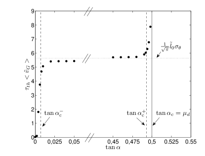
Figure 3: Velocity $<\tilde{v}_{G}>$ vs. angle $\alpha$ – The average velocity of the center of mass, $<\tilde{v}_{G}>$ depends only slightly on $\alpha$ (plateau) over a wide range of the incline angle typically from $\alpha_{\mathrm{c}}^{-}$ to $\alpha_{\mathrm{c}}^{+}$. Below $\alpha_{\mathrm{c}}^{-}$, $<\tilde{v}_{G}>$ vanishes for vanishing $\alpha$. Above $\alpha_{\mathrm{c}}^{+}$, $<\tilde{v}_{G}>$ drastically increases when $\alpha$ is increased and diverges for $\alpha=\alpha_{\mathrm{c}}$ ($\tilde{l}_{0}=10^{3}$, $\mu_{\mathrm{d}}$=0.5, $\overline{\mu}_{\mathrm{s}}$=0.6, $\sigma_{\mu}$ = 0.01 and $\sigma_{\theta}$ = 0.01).

III.1.2 Analysis

The results presented above can be qualitatively understood by simple arguments.

First, for $\alpha=0$, by symmetry, we expect $<\tilde{v}_{G}>=0$. This case has been extensively studied in Ref. geminard10 . The system ages and the center of mass experiences a sub-diffusive motion. Second, for $\alpha>\alpha_{\mathrm{c}}=\arctan(\mu_{d})$, if the system starts sliding as a whole, the $x$-component of the weight exceeds the dynamic friction force and the system accelerates. A finite average velocity is not defined in this case.

The most striking result, i.e., the plateau observed over a wide range of the incline angle ($\alpha_{\mathrm{c}}^{-}\lesssim\alpha\lesssim\alpha_{\mathrm{c}}^{+}$), can be easily understood by considering the mechanical stability of each of the sliders. Indeed, assuming that the values of the static friction coefficients $\mu_{\mathrm{s},1}$ and $\mu_{\mathrm{s},2}$ are close to each other, one can see that, because of the force $mg\,\sin(\alpha)$ due to the gravity, the lower (resp. upper) slider moves downwards when the system dilates (resp. contracts). As a consequence, if $\theta_{q+1}>\theta_{q}$ (the system dilates by $\Delta\theta\equiv\theta_{q+1}-\theta_{q}>0$), the resulting displacement of the center of mass is $\Delta\tilde{x}_{G}=\frac{1}{2}\Delta\tilde{x}_{2}\simeq\frac{1}{2}\tilde{l}_{0}\Delta\theta$. In the same way, if $\theta_{q+1}<\theta_{q}$ (the system contracts by $\Delta\theta<0$), $\Delta\tilde{x}_{G}=\frac{1}{2}\Delta\tilde{x}_{1}\simeq-\frac{1}{2}\tilde{l}_{0}\Delta\theta$. Thus, whatever the sign of $\Delta\theta$ (a contraction or a dilation), $\Delta\tilde{x}_{G}\simeq\frac{1}{2}\tilde{l}_{0}|\Delta\theta|$. Note that $\Delta\tilde{x}_{G}$ does not depend on the angle $\alpha$. Thus, when the system is subjected to periodic dilations from $\pm A_{\theta}$ to $\mp A_{\theta}$, the center of mass is displaced by $\Delta\tilde{x}_{G}\simeq\frac{1}{2}\tilde{l}_{0}(2A_{\theta})$ during ${\tau_{\mathrm{th}}}$ such that the average velocity of the system is given by:

$$\tau_{\mathrm{th}}<\tilde{v}_{G}>\,\simeq\tilde{l}_{0}A_{\theta}.$$ (13)

In the case of Gaussian fluctuations [Eq. (12)], taking into account the distribution $\psi(\theta)$, we estimate the average velocity of the center of mass for $\alpha_{\mathrm{c}}^{-}\lesssim\alpha\lesssim\alpha_{\mathrm{c}}^{+}$:

$$\tau_{\mathrm{th}}<\tilde{v}_{G}>\,\approx\frac{1}{\sqrt{\pi}}\tilde{l}_{0}\sigma_{\theta}.$$ (14)

The latter theoretical predictions (13) and (14) are in good agreement with the numerical results for large values of $A_{\theta}$ and $\sigma_{\theta}$ in a finite range of $\alpha$ (Fig. 3).

Let us focus on the critical angles $\alpha_{\mathrm{c}}^{-}$ and $\alpha_{\mathrm{c}}^{+}$ which limit the plateau. On the one hand, the plateau velocity is reached if the angle $\alpha$ is large enough ($\alpha\gtrsim\alpha_{\mathrm{c}}^{-}$) for the force due to the gravity to insure that the upper slider remains stable when the system dilates and, conversely, that the lower slider remains stable when the system contracts. For instance, for a dilation, the lower slider (the slider 2) destabilizes first if $f_{1\to 2}+mg\,\sin\alpha>\mu_{\mathrm{s},2}\,mg\,\cos\alpha$ [Eq. (10)] and $f_{2\to 1}+mg\,\sin\alpha>-\mu_{\mathrm{s},1}\,mg\,\cos\alpha$ [Eq. (8)]. The condition is thus, by summing the two inequalities, $\tan\alpha>\frac{1}{2}(\mu_{\mathrm{s},2}-\mu_{\mathrm{s},1})$. Taking into account the probability distribution $p(\mu_{\mathrm{s}})$, we deduce that the latter condition is generally fulfilled if $\tan\alpha>\tan\alpha_{\mathrm{c}}^{-}\equiv\sigma_{\mu}/\sqrt{2}$, which defines $\alpha_{\mathrm{c}}^{-}$ (Fig. 3).

On the other hand, the velocity of the system is larger than the plateau velocity if the motion of one slider can induce the motion of the second one ($\alpha\gtrsim\alpha_{\mathrm{c}}^{+}$). The angle $\alpha_{\mathrm{c}}^{+}$ can be estimated by considering, for instance, a dilation such that the slider 2 starts moving for $f_{1\to 2}+mg\,\sin\alpha>\mu_{\mathrm{s},2}\,mg\,\cos\alpha$ [Eq. (10)]. Provided that the slider 1 remains at rest, the force $f_{1\to 2}$ decreases by $\Delta f_{1\to 2}=2\,mg\,\cos\alpha\,(\mu_{\mathrm{s},2}-\mu_{\mathrm{d}})$ [by solving the equation (7)]. The slider 1 remains stable if $-f_{1\to 2}+mg\,\sin\alpha<\mu_{\mathrm{s},1}\,mg\,\cos\alpha$ [Eq. (8)], i.e. if $\tan\alpha<\mu_{\mathrm{d}}+{(\mu_{\mathrm{s},1}-\mu_{\mathrm{s},2})}/{2}$. We obtain a similar result by considering a contraction of the system. Thus, considering the width of the distribution $p(\mu_{\mathrm{s}})$ [Eq. (11)], we estimate that the second slider generally remains stable provided that $\tan\alpha<\tan\alpha_{\mathrm{c}}^{+}\equiv\mu_{\mathrm{d}}-\sigma_{\mu}/{\sqrt{2}}$, which defines $\alpha_{\mathrm{c}}^{+}$ (Fig. 3).

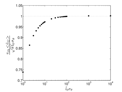
Figure 4: Velocity $<\tilde{v}_{G}>$ vs. typical amplitude $\sigma_{\theta}$ – In accordance with equation (17), the average velocity $<\tilde{v}_{G}>$ tends to the asymptote ${\tilde{l}_{0}}\sigma_{\theta}/(\sqrt{\pi}\tau_{\mathrm{th}})$ only in the limit $\sigma_{\theta}\gg\sigma_{\theta}^{*}$ (Here $\tilde{l}_{0}\sigma_{\theta}^{*}$ is about 0.4 whereas the asymptote is reached to within 1% for $\tilde{l}_{0}\sigma_{\theta}$ about 100, $\tilde{l}_{0}=10^{3}$, $\mu_{\mathrm{d}}$=0.5, $\overline{\mu}_{\mathrm{s}}$=0.6, $\sigma_{\mu}$ = 0.01 and $\tan{\alpha}$ = 0.25).

The simplistic reasoning proposed above leads to the prediction of a well-defined plateau between $\alpha_{\mathrm{c}}^{-}$ and $\alpha_{\mathrm{c}}^{+}$. However, a careful analysis of the numerical data reveals that $<\tilde{v}_{G}>$ slightly increases with the angle $\alpha$ even for large amplitudes $A_{\theta}$ or $\sigma_{\theta}$ (Fig. 3). To obtain the plateau values [Eq. (13)] or [Eq. (14)], we implicitly assumed that any variation of $\theta$ was enough for one of the conditions (8) and (10) to be fulfilled, which is not correct when a dilation is followed by a contraction (or conversely). In this case, taking into account that the stable and unstable sliders are swapped in Eqs. (8) and (10), we obtain $\Delta\tilde{x}_{G}\simeq\frac{1}{2}\Bigl{[}\tilde{l}_{0}|\Delta\theta|-2(\overline{\mu}_{\mathrm{s}}\cos{\alpha}-\sin{\alpha})\Bigr{]}$. The sliding distance is reduced by the fact that a minimum dilation is necessary to invert the direction of the frictional force. As a consequence, in the case of periodic cycling, the velocity is given by:

$$\tau_{\mathrm{th}}<\tilde{v}_{G}>\,\simeq\tilde{l}_{0}A_{\theta}-(\overline{\mu}_{\mathrm{s}}\cos{\alpha}-\sin{\alpha}),$$ (15)

which explains the mild increase of $<\tilde{v}_{G}>$ with $\alpha$ for $\tilde{l}_{0}A_{\theta}\gg 1$. The relation (15) holds valid provided that $A_{\theta}>A_{\theta}^{*}$ defined by:

$$A_{\theta}^{*}\equiv\frac{1}{\tilde{l}_{0}}(\overline{\mu}_{\mathrm{s}}\cos{\alpha}-\sin{\alpha}).$$ (16)

If the amplitude is smaller than $A_{\theta}^{*}$, the dilations are not sufficient to rearrange the system and $<\tilde{v}_{G}>=0$. In the case of Gaussian variations [Eq. (12)], a dilation (resp. contraction) is followed by a contraction (resp. dilation) in 2/3 of the timesteps. As a consequence, in a first approximation, the average velocity is given by

$$\tau_{\mathrm{th}}<\tilde{v}_{G}>\,\approx\frac{\tilde{l}_{0}}{\sqrt{\pi}}\sigma_{\theta}-\frac{2}{3}(\overline{\mu}_{\mathrm{s}}\cos{\alpha}-\sin{\alpha}).$$ (17)

where we assumed that all dilations are large enough to rearrange the system in each of the timesteps. The condition is reasonnably fulfilled when $\sigma_{\theta}$ is much larger than:

$$\sigma_{\theta}^{*}\equiv\frac{2\sqrt{\pi}}{3\tilde{l}_{0}}(\overline{\mu}_{\mathrm{s}}\cos{\alpha}-\sin{\alpha}).$$ (18)

Thus, for $\sigma_{\theta}\gg\sigma_{\theta}^{*}$, $<\tilde{v}_{G}>$ increases linearly with $\sigma_{\theta}$ [Eq. (17)]. When $\sigma_{\theta}$ is deacreased, even below $\sigma_{\theta}^{*}$, the dilations are always likely to rearrange the system and $<\tilde{v}_{G}>$ continuously decreases and vanishes only for $\sigma_{\theta}=0$ (Fig. 4).

III.2 Large systems: more than 2 sliders

Consider now a system consisting of N sliders connected by N-1 springs. It is important to notice that, for $N>2$, the system differs qualitatively from the system made of 2 sliders. Indeed, for $N>2$, the dilation can induce the motion of the sliders at both ends without, necessarily inducing, a displacement of the slider(s) at center. Thus, the successive dilations do not necessarily induce a displacement of the center of mass in average.

III.2.1 Numerical results

In order to account for the creep of the system along the slope we consider the position of the center of mass $\tilde{x}_{G}\equiv\frac{1}{N}\,\sum_{n=1}^{N}\tilde{x}_{n}$ as a function of time at the timesteps $t_{q}$ and report the average velocity $<\tilde{v}_{G}>$, for large amplitudes $A_{\theta}$ or $\sigma_{\theta}$, as a function of the incline angle $\alpha$ (Fig. 5). We observe that, for a small number $N$ of sliders, $<\tilde{v}_{G}>$ exhibits a series of plateaus: $<\tilde{v}_{G}>$ takes an almost constant value in a finite range of the incline angle $\alpha$. The number of plateaus increases when the number $N$ of sliders is increased. As expected, $<\tilde{v}_{G}>$ drastically increases when $\alpha$ approaches the critical angle $\alpha_{\mathrm{c}}$.

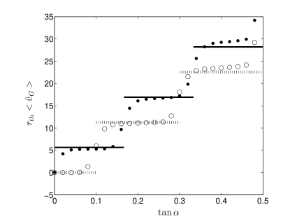
Figure 5: Velocity $<\tilde{v}_{G}>$ vs. incline angle $\alpha$ – The velocity $<\tilde{v}_{G}>$ exhibits a series of plateaus corresponding to constant velocities $v_{\mathrm{N,i}}^{*}$ above critical angles $\alpha_{\mathrm{N,i}}^{*}$. The number of plateaus increases with the number of sliders [dotted lines and open circles: $N=5$; full lines, and full circles: $N=6$. The plateau values (lines) are from Eq. (20)]. The velocity $<\tilde{v}_{G}>$ diverges when $\alpha$ approaches the critical angle $\alpha_{\mathrm{c}}$ ($\tilde{l}_{0}=10^{3}$, $\mu_{\mathrm{d}}$=0.5, $\overline{\mu}_{\mathrm{s}}$=0.6, $\sigma_{\mu}$ = 0.01 and $\sigma_{\theta}$ =0.01).

In the next section, we estimate theoretically the set of critical angles and the values of the corresponding plateau velocities in the large amplitude limit. In addition, we consider the dependence of the velocity on the amplitude of the temperature variations.

III.2.2 Analytic estimates

The behavior of the system can be understood by considering the motion of the internal sliders. Let us assume that, during a dilation of large amplitude, a given slider $i$ does not move whereas the sliders below move downwards and the sliders above move upwards. In the same way, let us assume that during a large contraction, a given slider $j$ does not move whereas the sliders above move downwards and the sliders below move upwards. If the incline angle $\alpha$ is large enough, the sliders $i$ and $j$ differ (with $i<j$). In this case, the internal displacements result in a reptation of the entire system along the incline as already described in the framework of the continuous models moseley ; bouasse ; tamburi74 .

Let us first determine the critical angle $\alpha_{\mathrm{N,i}}^{*}$ above which the slider $i$, previously at rest, starts moving downwards during a dilation, the slider $i-1$ remaining at rest instead. Thus, let us first consider that the slider $i$ remains at rest. We assume, in a first approach, that the dilation rate is large enough for the sliders in motion to slide continuously such that they are submitted to the dynamical frictional force $\pm\mu_{\mathrm{d}}mg\cos\alpha$. The condition is fulfilled provided that $\dot{\theta}\gg\Delta\mu/\tilde{l}_{0}\tau_{\mathrm{dyn}}$ where we define $\Delta\mu\equiv\mu_{\mathrm{s}}-\mu_{\mathrm{d}}$. In addition, the dilation must be large enough for all the downstream sliders to move downwards and all the upstream sliders to move upwards. We shall later discuss this assumption. In this case, neglecting the inertia, one can indeed write the forces exerted by the slider $i$ on the sliders $i-1$ and $i+1$:

$$f_{i\to i-1}+(i-1) (mg\sin\alpha+\mu_{\mathrm{d}}mg\cos\alpha)=0$$

$$f_{i\to i+1}+(N-i) (mg\sin\alpha-\mu_{\mathrm{d}}mg\cos\alpha)=0$$

Considering the condition for the stability of the slider $i$,

$$|f_{i-1\to i}+f_{i+1\to i}+mg\sin\alpha|<\mu_{\mathrm{d}}mg\cos\alpha,$$

we obtain that the slider $i$ starts moving downwards above the critical angle $\alpha_{\mathrm{N,i}}^{*}$ given by:

$$\tan\alpha_{N,i}^{*}=\mu_{\mathrm{d}}\Bigl{[}1-2\,\frac{i-1}{N}\Bigr{]}+\frac{\Delta\mu}{N}.$$ (19)

Note that $\alpha_{\mathrm{N,i}}^{*}$ is a decreasing function of $i$ such that the slider $i-1$ remains stable for $\alpha_{\mathrm{N,i}}^{*}<\alpha<\alpha_{\mathrm{N,i-1}}^{*}$.

Let us now consider a contraction of the same system. Assuming that for the chosen value of $\alpha$, the slider $i$ is at rest during the dilation, considering that the slider $j$ remains at rest during the contraction, we write:

$$f_{j\to j-1}+(j-1) (mg\sin\alpha-\mu_{\mathrm{d}}mg\cos\alpha)=0$$

$$f_{j\to j+1}+(N-j) (mg\sin\alpha+\mu_{\mathrm{d}}mg\cos\alpha)=0$$

Considering the stability of the slider $j$, replacing $\alpha$ by the critical value $\alpha_{\mathrm{N,i}}^{*}$, we obtain that for $\alpha>\alpha_{N,i}^{*}$ the slider $j=N+1-i$ starts moving downwards such that the slider $j+1$ is then at rest.

In summary, for $\alpha_{\mathrm{N,i}}^{*}<\alpha<\alpha_{\mathrm{N,i-1}}^{*}$, the slider $i-1$ remains stable during the dilation and the slider $j+1$ remains stable during the contraction of the system. Accordingly, we can write the displacements of any slider $n$, for a dilation $\Delta\tilde{x}_{\mathrm{n}}=[n-(i-1)]\,\tilde{l}_{0}\Delta\theta^{+}$ ($\Delta\theta^{+}>0$), for a contraction $\Delta\tilde{x}_{\mathrm{n}}=[n-(j+1)]\,\tilde{l}_{0}\Delta\theta^{-}$ ($\Delta\theta^{-}<0$). For a cycle $\Delta\theta^{+}=-\Delta\theta^{-}=2A_{\theta}$, one obtains the total displacement $\Delta\tilde{x}_{\mathrm{n}}=2(N+3-2i)\tilde{l}_{0}A_{\theta}$ for a total duration $2\,\tau_{\mathrm{th}}$. Note that $\Delta\tilde{x}_{\mathrm{n}}$ does not depend on $n$ and that the associated velocity of the center of mass is simply

$$\tau_{\mathrm{th}}v_{\mathrm{N,i}}^{*}=(N+3-2i)\,\tilde{l}_{0}A_{\theta}.$$ (20)

We thus expect, for cycles of amplitude $A_{\theta}$, the plateau velocity $v_{\mathrm{N,i}}^{*}$ for $\alpha_{\mathrm{N,i}}^{*}<\alpha<\alpha_{\mathrm{N,i-1}}^{*}$ and $1<i<(N+3)/2$ (note that, for $i=1$, $\alpha_{\mathrm{N,1}}^{*}$ corresponds to the critical angle of avalanche $\alpha_{c}$). For Gaussian temperature variations $A_{\theta}$ must be replaced by $\sigma_{\theta}/\sqrt{\pi}$ so that $\tau_{\mathrm{th}}v_{\mathrm{N,i}}^{*}=(N+3-2i)\,\tilde{l}_{0}\sigma_{\theta}/\sqrt{\pi}$ in this case. We observe in Fig. 5 that the equations (19) and (20) give good estimates of the transitions and plateau velocities.

When a contraction follows a dilation (or conversely), a compression (resp. dilation) wave propagates from both ends inwards. Equation (20) is correct provided that the amplitude $A_{\theta}$ is larger than a critical amplitude $A_{\theta}^{*}$, such that the temperature variations induce the motion of all the sliders in the chain, which can be assessed in the following way: For $\alpha_{\mathrm{N,i}}^{*}<\alpha<\alpha_{\mathrm{N,i-1}}^{*}$ and $A_{\theta}>A_{\theta}^{*}$, during a dilation, the slider $i-1$ pushes all the sliders below downwards so that:

$$f_{i-1\to i}+[N-(i-1)](\sin\alpha-\mu_{\mathrm{d}}\cos\alpha)=0$$ (21)

Note that during the dilation the sliders $i$ to $j$ are moving downwards so that the frictional force is already oriented upwards. During the contraction that follows, the sliders $1$ to $j$ move downwards provided that the contraction wave propagating from the upper end reaches the slider $i-1$. Let us now denote $\Delta\theta^{*}$ the corresponding dilation. For $\Delta\theta^{*}$, the slider $i-1$, which is still at rest, pulls all the sliders above downwards so that:

$$f_{i-1\to i-2}+(i-2)(\sin\alpha-\mu_{\mathrm{d}}\cos\alpha)=0.$$

The sliders $i-1$ and $i$ being still at rest, we get from equation (21),

$$f_{i\to i-1}=[N-(i-1)](\sin\alpha-\mu_{\mathrm{d}}\cos\alpha)-\tilde{l}_{0}\Delta\theta^{*}$$

The temperature variation induces the motion of the entire chain provided that

$$f_{i\to i-1}+f_{i-2\to i-1}+\sin\alpha-\mu_{\mathrm{s}}\cos\alpha>0$$

which leads to $-\tilde{l}_{0}\Delta\theta^{*}>N(\sin\alpha-\mu_{\mathrm{d}}\cos\alpha)-\Delta\mu\cos\alpha$ (remember here that $\Delta\theta^{*}<0$). Within a cycle, the amplitude of a contraction being $\Delta\theta=-2A_{\theta}$ and the argument developped above holding true for a dilation following a contraction, we obtain the minimal amplitude leading to the reptation of the chain:

$$A_{\theta}^{*}=\frac{N}{2\tilde{l}_{0}}(\mu_{\mathrm{d}}\cos\alpha-\sin\alpha)$$ (22)

where we assumed $\Delta\mu/N\ll 1$. Note that $A_{\theta}^{*}$ is independent of the position of the steady slider ($i$ or $j$) and proportional to the number $N$ of sliders in the chain. We can thus write, for finite amplitudes,

$$\tau_{\mathrm{th}}v_{\mathrm{N,i}}^{*}=(N+3-2i)\,\tilde{l}_{0}\Bigl{[}A_{\theta}-\frac{N}{2\tilde{l}_{0}}(\mu_{\mathrm{d}}\cos\alpha-\sin\alpha)\Bigr{]}.$$ (23)

The equation (23) is in excellent agreement with the numerical results even when the static and dynamical frictional coefficients are not equal ($\Delta\mu\neq 0$, Fig. 6). We thus also deduce from these observations that the average velocity is not sensitive to the width $\sigma_{\mu}$ of the distribution of the static frictional coefficient.

Figure 6: Velocity $<\tilde{v}_{G}>$ vs. amplitude $A_{\theta}$ or $\sigma_{\theta}$ – For temperature cycles (open circles), $<\tilde{v}_{g}>$ increases linearly with the amplitude $A_{\theta}$ above a critical amplitude $A_{\theta}^{*}$ in agreement with the equation (23) [continuous line]. For random temperature variations (full circles), $<\tilde{v}_{g}>$ increases significantly above a critical amplitude $\sigma_{\theta}^{*}$ of the temperature variations and reaches a linear asymptote for $\sigma_{\theta}\gg\sigma_{\theta}^{*}$ in agreement with the equation (24) [continuous line. We remind that the asymptote is reached only when $\sigma_{\theta}\gg\sigma_{\theta}^{*}$]. Random temperature variations thus lead to a smoother transition but do not change the qualitative behavior of the system ($N=30$, $\tilde{l}_{0}=10^{3}$, $\mu_{\mathrm{d}}$=0.5, $\mu_{\mathrm{s}}$=0.6, $\sigma_{\mu}$ = 0.01, and $\tan\alpha=0.25$).

In addition, the same qualitative behavior is expected, when the system is submitted to random temperature variations. In Fig. 6, we observe that equation (23) agrees with the numerical results, provided that the amplitude $A_{\theta}$ is replaced by $\sigma_{\theta}/\sqrt{\pi}$ and $A_{\theta}^{*}$ by $\sigma_{\theta}^{*}=\frac{2}{3}\sqrt{\pi}A_{\theta}^{*}$ so that:

$$\tau_{\mathrm{th}}v_{\mathrm{N,i}}^{*}=(N+3-2i)\,\tilde{l}_{0}\Bigl{[}\frac{\sigma_{\theta}}{\sqrt{\pi}}-\frac{N}{3\tilde{l}_{0}}(\mu_{\mathrm{d}}\cos\alpha-\sin\alpha)\Bigr{]}$$ (24)

for random temperature variations.

IV Discussion

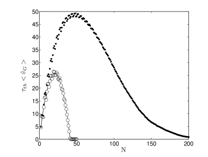
Figure 7: Velocity $<\tilde{v}_{G}>$ vs. number of sliders $N$ – For temperature cycles (open circles) and random temperature variations (full circles), $<\tilde{v}_{g}>$ exhibits a non-monotonic behavior as a function of $N$. For small $N$, $<\tilde{v}_{g}>$ increases because of the increase of the size of the system; for large $N$, $<\tilde{v}_{g}>$ decreases because of the increase of critical amplitude $A_{\theta}^{*}$ or $\sigma_{\theta}^{*}$. For temperature cycles, the numerical results are in excellent agreement with the equation (23) (continuous line). Note however the dispersion of the numerical points for small $N$ which is due to the fact that, at a given amplitude $A_{\theta}$, $<\tilde{v}_{g}>$ corresponds to discrete plateau values which are not accounted for by the equation (23) when considering continuous values of $\alpha$ ($\tilde{l}_{0}=10^{3}$, $\mu_{\mathrm{d}}$=0.5, $\overline{\mu}_{\mathrm{s}}$=0.6, $\sigma_{\mu}$ = 0.01, $A_{\theta}$ = 0.005 or $\sigma_{\theta}=0.005\sqrt{\pi}$ and $\tan\alpha=0.25$).

In the continuous description proposed by Moseley and Bouasse moseley ; bouasse , the elasticity of the material was neglected which led to the conclusion that the creep velocity was proportional to the amplitude of the temperature variations. The introduction of the elastic effects leads to the conclusion that the temperature variations induce the creep of the system only if their amplitude is large enough, as already proposed by Croll. However, note that the critical value given by the equation (22) differs from the result proposed in croll09 . The difference comes from the fact that Croll considered that the system was free of stress at the beginning of each phase of a cycle (dilation or contraction). In our approach, each dilation (resp. contraction) follows a contraction (resp. dilation) and the frictional force is initially non zero, mobilized in the opposite direction. Considering that our chain of sliders model a solid of mass $M$, length $L$, cross section $S$ made of a material having a Young modulus $Y$ and a density $\rho$ creeping along an incline, one can estimate from equation (20), provided that $k=NYS/L$,

$$\tau_{\mathrm{th}}v_{G}=L\frac{\tan\alpha}{\mu_{\mathrm{d}}}\Bigl{[}A_{\theta}-\frac{g\rho L}{2Y}(\mu_{\mathrm{d}}\cos\alpha-\sin\alpha)\Bigr{]}.$$ (25)

We thus obtain that the creep velocity is independent of the number $N$ of contacts. The minimum amplitude of the temperature changes that produce the creep of the system along the incline can be written:

$$\Delta T^{*}=\frac{g\rho L}{2Y\kappa}(\mu_{\mathrm{d}}\cos\alpha-\sin\alpha).$$ (26)

Thus, for a given $L$, the system is thus more likely to creep along the incline for a larger Young modulus $Y$, a larger thermal expansion coefficient $\kappa$ and a larger angle $\alpha$. Note again that the stability of the system does not depend on the number $N$ of contacts. Typically, with $L=1$ cm, $Y\sim 100$ GPa and $\rho\sim 10^{4}$ kg.m^-3, we estimate that relative dilations of about $10^{-8}$ are enough to make the system creep. Such dilations, which correspond to temperature changes of about $\Delta T\sim 1$ mK, are difficult to avoid and, in general, any frictional contact between two macroscopic solids cannot be considered as perfectly static.

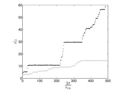
Figure 8: Position $<\tilde{x}_{G}>$ vs. time ${t}$ – For $A_{\theta}\simeq A_{\theta}^{*}$, the system exhibits an irregular dynamics even when temperature cycles are imposed. Note that fast creep can be followed by long quiescent periods as observed for $A_{\theta}=1.01A_{\theta}^{*}$ (black) and $A_{\theta}=0.99A_{\theta}^{*}$ (grey) for $A_{\theta}^{*}\simeq 3.6~{}10^{-3}$ ($N=30$, $\tilde{l}_{0}=10^{3}$, $\mu_{\mathrm{d}}$=0.5, $\mu_{\mathrm{s}}$=0.6, $\sigma_{\mu}$ = 0 and $\tan\alpha=0.25$).

The second practical situation mentionned in the introduction is the creep of granular material induced by temperature changes geminard03 ; chen06 ; chen09 ; divoux08 ; divoux09 ; divoux09t ; divoux10 . In this case, the length $l_{0}$ would account for the typical grain size, $k$ for the rigidity associated with the grain-grain contact and $N$ for the typical number of grains in one typical dimension $L=Nl_{0}$ of the system. It is then particularly interesting to consider the dependence of the typical creep velocity on the number $N$ [Eq. (23), Fig. 7]. For a given amplitude of the temperature variations, $<\tilde{v}_{g}>$ exhibits a non-monotonic behavior as a function of $N$, increasing linearly with $N$ for small $N$ and decreasing for large $N$ because of the increase of the critical amplitude of the temperature variations likely to induce the creep [Eq. (22)]. For temperature cycles, from equation (22), $<\tilde{v}_{g}>$ is expected to vanish for $N>{2\tilde{l}_{0}}A_{\theta}/(\mu_{\mathrm{d}}\cos\alpha-\sin\alpha)$ whereas random temperature variations are expected to be always likely to produce creep.

Let us now focus on the dynamics of the system subjected to temperature cycles of amplitude close to $A_{\theta}^{*}$ (Fig. 8). We observe that, for $A_{\theta}$ close to $A_{\theta}^{*}$ (above and below $A_{\theta}^{*}$) the system creeps in an irregular manner. The position of the center of mass, $\tilde{x}_{\mathrm{G}}$, exhibits a series of rapid variations (jumps), separated by periods of time during which the system is apparently at rest. This latter conclusion holds true even if the value of the static frictional coefficient is well-defined, i.e. even for $\sigma_{\mu}=0$. Thus, for $A_{\theta}$ approaching $A_{\theta}^{*}$, one observes a transition from a continuous creep regime, during which $\tilde{x}_{\mathrm{G}}$ decreases at each cycle, to the irregular creep regime. The transition is reminiscent of the transition between a continuous-flow and an intermittent-flow regime, observed when the amplitude of the temperature cycles imposed to a granular column is decreased divoux08 ; divoux09 ; divoux09t ; divoux10 . The experimental and theoretical systems are very different but there are some common aspects like the frictional contact between the particles that are in a limited number $N$. We can however attempt to estimate the critical amplitude $A_{\theta}^{*}$ expected from the model for a column (diameter 1 cm) of glass beads (typically 500 $\mu$m in diameter). The elasticity of the system is due to the Hertz contact between the grains and we can estimate that the stiffness $k$ depends on the pressure. Denoting $\delta$ the penetration distance and $R$ the radius of the grains, we can write $k\sim Y(R\delta)^{1/2}$. For an infinite vertical column, because of Janssen effect, one can estimate the local pressure $P\sim\rho gD$, where $D$ stands for the diameter of the column and $\rho$ for the density of glass. Writing that the force applied to the grains $k\delta\sim PR^{2}$, we get $k\sim R[\rho gDY^{2}]^{1/3}$. From equation (22), with $l_{0}\sim 2R$ and $N\sim D/2R$, we estimate $A_{\theta}^{*}\sim(\rho gD/Y)^{2/3}$. Note first that the result does not depend on the size of the grains and, thus, not on the number of grains in the diameter of the column. Second, with $\rho\sim 2\,10^{3}$, $D\sim 1$ cm and $Y\sim 20$ GPa, we obtain that $A_{\theta}^{*}\sim 5\,10^{-6}$ and, thus, with $\kappa\simeq 3\,10^{-6}$ K^-1 for glass, that a transition between the continuous- and the irregular-flow regimes is expected for amplitudes of the temperature variations of the order of 1 K. The latter value is interestingly close to the experimental value which is of about 3 K divoux08 . Even if the good agreement between the theoretical estimate and the experimental values might be accidental, we think that the comparison between our model and the granular column is worth to be mentionned.

V Conclusion

We reported on the detailed behavior of a frictional system subjected to thermal dilations. We observed that for a small number of sliders in the chain and large amplitude of the dilations, the ’reptation’ velocity of the center of mass exhibits a series of plateaus as a function of the incline angle. In the limit of an infinite number of sliders and large amplitudes, we recover former results obtained for the creep of a solid on an incline. Because of the elasticity of the material, the creep velocity is expected to vanish for a finite value when the amplitude of the cycles is decreased. We obtain an expression of the critical velocity which slighly differs from former results.

Finally, for a finite number of sliders, we observe, numerically, that the system experiences an irregular trajectory, the center of mass sliding rapidly between quiescent, rather long, periods of time even if the system is subjected to periodic cycling. The transition between the continuous and the irregular creep depends on the size of the system. The irregular creep is reminiscent of recent observations of the irregular compaction of granular matter under the action of periodic temperature changes. The systems are very different but we do believe that the study of this specific regime will provide us with interesting clues for the understanding of the peculiar behavior of granular matter. The latter study will be the subject of a further publication.

- (1) J.B. Knight et al., Phys. Rev. E 51 (1995) 3957 .
- (2) P. Philippe and D. Bideau, Eur. Phys. Lett. 60, (2002) 677.
- (3) O. Pouliquen et al., Phys. Rev. Lett. 91, (2003) 014301.
- (4) L. Vanel and E. Clément, Eur. Phys. J. B 11, (1999) 525.
- (5) E. Clément et al, Proceedings of the IIIrd Intern. Conf. on Powders & Grains (Balkema, Rotterdam, 1997)
- (6) P. Claudin and J.-P. Bouchaud, Phys. Rev. Lett. 78, (1997) 231.
- (7) J.-C. Géminard, Habilitation à Diriger des Recherches, Quelques propriétés mécaniques des matériaux granulaires immergés, Université Joseph Fourier - Grenoble I (2003).
- (8) K. Chen, J. Cole, C. Conger, J. Draskovic, M. Lohr, K. Klein, T. Scheidemantel and P. Schiffer, Nature 442, 257 (2006).
- (9) K. Chen, A. Harris, J. Draskovic and P. Schiffer, Gran. Matt. 11, 237 (2009).
- (10) T. Divoux, H. Gayvallet and J.-C. Géminard, Phys. Rev. Lett. 101 (2008) 148303.
- (11) T. Divoux, I. Vassilief, H. Gayvallet and J.-C. Géminard, AIP Conference Proceedings (Eds. M. Nakagawa and S. Luding), 6th International Conference on the Micromechanics of Granular Media (Golden, CO, 2009).
- (12) T. Divoux, PhD, Bruit et fluctuations dans les écoulements de fluides complexes, Ecole Normale Supérieure de Lyon (2009).
- (13) T. Divoux, Papers in Physics 2, 020006 (2010).
- (14) H. Moseley, The mechanical principles of engineering and architecture, Eds. Wiley & Halstead, New York (1853).
- (15) H. Bouasse, Statique, Bibliothèque Scientifique de l’Ingénieur et du Physicien, pp. 259-261 (1920) .
- (16) J. G.A. Croll, Proc. R. Soc. A 465, 791-807 (2009).
- (17) A. J. Tamburi, GSA bulletin, 85, 351-356 (1974).
- (18) B. N. J. Persson, J. Phys.: Condens. Matter 22, 265004 (2010).
- (19) T. Baumberger and C. Caroli, Adv. Phys. 55, 279-348 (2006).
- (20) J.-C. Géminard and E. Bertin, Phys. Rev. E 82, 056108 (2010).
- (21) M. P. Allen and D. J. Tildesley, Computer Simulation of Liquids, Clarendon, Oxford, 1987.