On the temperature dependence of ballistic Coulomb drag in nanowires

Abstract

We have investigated within the theory of Fermi liquid dependence of Coulomb drag current in a passive quantum wire on the applied voltage $V$ across an active wire and on the temperature $T$ for any values of $eV/k_{B}T$. We assume that the bottoms of the 1D minibands in both wires almost coincide with the Fermi level. We come to conclusions that 1) within a certain temperature interval the drag current can be a descending function of the temperature $T$; 2) the experimentally observed temperature dependence $T^{-0.77}$ of the drag current can be interpreted within the framework of Fermi liquid theory; 3) at relatively high applied voltages the drag current as a function of the applied voltage saturates; 4) the screening of the electron potential by metallic gate electrodes can be of importance.

Coulomb drag predicted by Pogrebinskii POG (see also Price Price ) is a phenomenon directly associated with Coulomb interaction of the electrons in a semiconductor. Perpetually advancing progress in semiconductor lithography technique has provided extensive investigation of this effect between 2D electron layers separated by hundreds or tens of angstroms and supported interest to this field (see, e.g. Rojo , where a number of papers dealing with the Coulomb drag between two 2D layers is discussed).

Coulomb drag effect for two parallel quantum wires in the ballistic regime has been investigated by Gurevich, Pevzner and Fenton in Ref. GPF, for $eV\,\ll\,k_{B}T$. This case may be called linear as the drag current is a linear function of the applied voltage $V$. The authors of the present paper treated in Ref. GM_Nonohmic_Coul, a nonlinear case where $eV\,\gtrsim\,k_{B}T$. In both cases the Fermi energy $\mu$ was assumed to be much larger than $k_{B}T$. As is well known, under this condition the transport phenomena are determined by a stripe of the width $k_{B}T$ near the Fermi level. This means that the drag current $J_{\rm drag}$ should have a maximum provided the positions of these stripes in both quantum wires coincide. For identical wires (the case treated in Refs. GPF ; GM_Nonohmic_Coul ) this requirement means coincidence of the bottoms of 1D bands of transverse quantization. Under these conditions $J_{\rm drag}$ goes up with temperature.

One encounters an entirely different situation provided the Fermi level is near the bottom of a 1D band. If this is the case for two bands in both wires all the electrons of these bands can take part in the electron-electron collisions. The very effect of drag is strongly dependent on the transferred (quasi)momentum $p_{\rm tr}$ in the course of interwire Coulomb scattering of electrons. The number of electrons involved goes down with $p_{\rm tr}$ whereas the interaction responsible for the drag goes up and its influence is predominant for $J_{\rm drag}$. Our purpose is to investigate this situation. In other words, we assume that

$$|\mu_{n}|\lesssim k_{B}T,\quad\mu_{n}\equiv\mu-\varepsilon_{n}(0)$$ (1)

where $\varepsilon_{n}(0)$ is the position of the bottom of $n$th 1D band (a result of the transverse quantization) and $\mu$ is the chemical potential. In the discussion of the experimental situation we will use the findings of Refs. DVRPRM and DZRKVN (see also the review paper DGKN ). As is seen in these works, the drag voltage peaks occur just where the quantized conductance of the drive (active) wire rises between the plateaus, i.e. the maximum of the drag effect occurs provided the 1D bands of the two quantum wires are aligned (i. e. their bottoms coincide within the accuracy of $\lesssim k_{B}T$) and Fermi quasimomenta are small. First two peaks are well pronounced. First of them corresponds to alignment of the two ground 1D bands in both wires. The second one corresponds to alignment of the ground (first) 1D band of the passive (drag) wire and the second 1D band of the drive wire.

It was found that the temperature dependence of the drag current can be described by the law $\sim\,T^{-0.77}$ in the temperature interval from $60$ mK to $1$ K. The authors of these papers highlight this temperature dependence claiming that the power-law temperature dependence of the drag resistance is a signature of the Luttinger liquid state. The authors of PBT evidently share the same opinion, claiming that for coupled Fermi liquid systems the drag resistance always is an increasing function of temperature.

In this paper we will argue that the situation is not so simple, and the temperature dependence observed on experiment can be explained within the Fermi liquid approach.

Experimentally found magnitudes of the drag resistance are of order of hundreds Ohms or even smaller and one should provide a special explanation for the weakness of the interwire electron-electron interaction. We believe that it is due to the screening of Coulomb interaction by the gates. Such screening has not been taken into consideration so far. In Ref.  GM_Nonohmic_Coul the following equation has been derived for the drag current (see Eq. (13) in GM_Nonohmic_Coul )

$$J_{\rm drag}=-2e\sinh{\left({eV\over{2k_{B}T}}\right)}{2\pi\over{\hbar}}{mL\over{2\pi\hbar}}\left({2L\over{2\pi\hbar}}\right)^{2}\left({2e^{2}\over{\kappa L}}\right)^{2}\sum_{nn^{\prime}}\int_{0}^{\infty}dp\int_{0}^{\infty}dp^{\prime}\displaystyle{g_{nn^{\prime}}(p+p^{\prime})\over{p+p^{\prime}}}{\cal Q},$$ (2)

where

$${\cal Q}=\exp{\varepsilon^{(1)}_{np}-\mu\over k_{B}T}\exp{\varepsilon^{(2)}_{n\prime p\prime}-\mu\over k_{B}T}f(\varepsilon^{(1)}_{np}-\mu)f\left(\varepsilon^{(2)}_{n^{\prime}p^{\prime}}-\mu-{eV\over 2}\right)f(\varepsilon^{(1)}_{np^{\prime}}-\mu)f\left(\varepsilon^{(2)}_{n^{\prime}p}-\mu+{eV\over 2}\right),$$ (3)

Here $f(\varepsilon-\mu)$ is the Fermi function and $\kappa$ is the dielectric susceptibility.

The unscreened Coulomb interaction matrix element squared $g_{nl}(p+p^{\prime})$ can be written as $\left[K_{0}(d(p+p^{\prime})/\hbar)\right]^{2}$ provided the widths of the wires are much smaller than the interwire distance $d$. Here $K_{0}(s)$ is the MacDonald function. Using the random phase approximation one can straightforwardly take into consideration the screening by the gates as well as by the quantum wires themselves. The resulting equation being, however, too cumbersome, we will take into account the screening only by the gates treating them as a single plane. As for the contribution of 1D wires to the screening, we will neglect it. As a result, we get for the screened Coulomb interaction

$$U_{s}(\omega,q_{x})=\int\frac{d{\bf q}_{\perp}}{(2\pi)^{2}}C_{n}({\bf q}_{\perp})U_{\bf q}C_{l}(-{\bf q}_{\perp})+$$

$$+\int\frac{d{\bf q}_{\perp}}{(2\pi)^{2}}C_{n}({\bf q}_{\perp})U_{\bf q}\int\frac{dq_{z}^{\prime}}{2\pi}C_{l}(-q_{y},-q_{z}^{\prime})U_{q_{x},q_{y},q_{z}^{\prime}}\frac{\Pi^{R}_{\omega}({q_{x},q_{y}})}{1-\Pi^{R}_{\omega}({q_{x},q_{y}})U(q_{x},q_{y})}$$ (4)

where $C_{n}({\bf q}_{\perp})=\langle n|e^{i{\bf q}_{\perp}{\bf r}_{1\perp}}|n\rangle$ and $C_{l}({\bf q}_{\perp})=\langle l|e^{i{\bf q}_{\perp}{\bf r}_{2\perp}}|l\rangle$. Here $|n\rangle$ and $|l\rangle$ are the transverse wave functions of the first and second quantum wires. Precisely,

$$|n\rangle=\phi_{np}({\bf r}_{\perp}),\quad{\bf r}_{\perp}\longleftrightarrow y,z$$

are the wave function describing the transverse quantization. $U_{\bf q}=4\pi e^{2}/\kappa q^{2}$ is the Fourier transform of the 3D Coulomb potential, $U(q_{x},q_{y})=\int\,dq_{z}\,U_{\bf q}/2\pi$. Polarization operator $\Pi^{R}(\omega,q_{x},q_{y})$ for a 2D layer can be found in Ref. Stern . We assume that the gate electrodes are made of a metal where the period of plasma vibration is much shorter than any characteristic time of a semiconductor. Therefore we will deal only with a static as well as long wave limit of this operator. In this limit it is reduced to the 2D electron density of states.

We assume that the gates are in the plane $z=0$, two quantum wires parallel to the plane (and oriented along the $x$-axis) are displaced by the same distance $z_{0}$, the interwire distance being $d$. For the electrons with coordinates $x,0,z_{0}$ and $x^{\prime},d,z_{0}$, belonging to two wires

$$U_{s}(\omega,x-x^{\prime})=e^{2}\int\frac{e^{-iq_{y}d-iq_{x}(x-x^{\prime})}dq_{y}dq_{x}}{2\pi\sqrt{q_{x}^{2}+q_{y}^{2}}}+$$

$$+e^{2}\int\frac{e^{-iq_{y}d-iq_{x}(x-x^{\prime})}dq_{y}dq_{x}}{2\pi(q_{x}^{2}+q_{y}^{2})}\frac{2\pi e^{2}\Pi^{R}_{\omega}({q_{x},q_{y}})e^{-2\sqrt{q_{x}^{2}+q_{y}^{2}}z_{0}}}{1-2\pi e^{2}\Pi^{R}_{\omega}({q_{x},q_{y}})/\sqrt{q_{x}^{2}+q_{y}^{2}}}.$$ (5)

In the static case we arrive at a simple result

$$U_{s}(x-x^{\prime})=\frac{e^{2}}{\sqrt{(x-x^{\prime})^{2}+d^{2}}}-\frac{e^{2}}{\sqrt{(x-x^{\prime})^{2}+d^{2}+(2z_{0})^{2}}},$$ (6)

the second term here describes the action of an ”image” (we assume that $z_{0}$ is bigger than the Bohr radius).

Therefore we get for the drag current instead of (2)

$$J_{\rm drag}=-\frac{2e^{5}mL}{\pi^{2}\hbar^{4}\kappa^{2}}\left(\frac{z_{0}}{d}\right)^{4}\left(\frac{d}{\hbar}\right)^{2}\sinh{\frac{eV}{2k_{B}T}}\sum_{nl}\int_{0}^{\infty}dp\int_{0}^{\infty}dp^{\prime}(p+p^{\prime})K_{1}^{2}\left(d(p+p^{\prime})/\hbar\right){\cal Q},$$ (7)

where now

$${\cal Q}=\frac{1}{\cosh{[(p^{2}-p_{n}^{2})/4mk_{B}T]}\cosh{[(p^{2}-p_{n}^{2}+meV-2m\varepsilon_{nl})/4mk_{B}T]}}$$

$$\times\frac{1}{\cosh{[(p^{\prime 2}-p_{n}^{2})/4mk_{B}T]}\cosh{[(p^{\prime 2}-p_{n}^{2}-meV-2m\varepsilon_{nl})/4mk_{B}T]}}$$

and

$$\varepsilon_{nl}=\varepsilon_{n}-\varepsilon_{l}.$$

Here we have defined the Fermi quasimomentum $p_{n}=\sqrt{2m(\mu-\varepsilon_{n})}$ while $\varepsilon_{n}$ and $\varepsilon_{l}$ are the positions of 1D band bottoms. In what follows we will assume that

$$d\gg z_{0},$$ (8)

i. e. the spacing $d$ between the quantum wires is larger than their distance $z_{0}$ to the gates.

Now

$$K_{0}\left(d\frac{p+p^{\prime}}{\hbar}\right)-K_{0}\left(\sqrt{1+(2z_{0}/d)^{2}}d\frac{p+p^{\prime}}{\hbar}\right)\simeq\,2\left(\frac{z_{0}}{d}\right)^{2}d\frac{p+p^{\prime}}{\hbar}K_{1}\left(d\frac{p+p^{\prime}}{\hbar}\right).$$ (9)

The scale of variation of $Q$ as a function of $p$ and $p^{\prime}$ is the thermal momentum $\sqrt{4mk_{B}T}$. At the same time $(p+p^{\prime})K_{1}^{2}\left(d(p+p^{\prime})/\hbar\right)$ is a rapidly decreasing function, the scale of its variation is $\hbar/d$. For

$$\hbar/d\,\ll\,\sqrt{4mk_{B}T}$$

one can take out of the integral all the slowly varying functions keeping as the integrand only $(p+p^{\prime})K_{1}^{2}\left(d(p+p^{\prime})/\hbar\right)$. For $p_{n}\geq\,\hbar/d$ in the case of 1D band alignment in two wires

$$\varepsilon_{n}\approx\varepsilon_{l}$$

we can retain the contribution only of these 1D bands in the sum and get

$$J_{\rm drag}=J_{0}\frac{\sinh{[eV/2k_{B}T]}}{\cosh^{2}{[p_{n}^{2}/4mk_{B}T]}\cosh{[(p_{n}^{2}-meV)/4mk_{B}T]}\cosh{[(p_{n}^{2}+meV)/4mk_{B}T]}},$$ (10)

where

$$J_{0}=-\frac{3e^{5}mL}{16\hbar^{3}d\kappa^{2}}\left(\frac{z_{0}}{d}\right)^{4}.$$ (11)

Here we have made use of the equation

$$\int_{0}^{\infty}dx\int_{0}^{\infty}dy\,(x+y)K_{1}^{2}(x+y)=\frac{3\pi^{2}}{32}.$$ (12)

The temperature dependence in the considered region of temperatures as well as the dependence on the applied voltage is given by Eq. (10). Within a comparatively big temperature interval the drag is a descending function of temperature. At smaller temperatures it reaches a maximum. At small applied voltages we have

$$J_{\rm drag}=J_{0}\frac{eV}{2k_{B}T}\frac{1}{\cosh^{4}{[p_{n}^{2}/4mk_{B}T]}},$$ (13)

a linear dependence on $V$, for bigger voltages the drag current saturates at

$$J_{\rm drag}=2J_{0}\frac{1}{\cosh^{2}{[p_{n}^{2}/4mk_{B}T]}}.$$ (14)

We wish to emphasize that the screening has nothing to do with the temperature dependence. The small factor $(z_{0}/d)^{4}$ indicates that the screening can be important as it can explain the magnitude of the effect (without regard of the screening the theory would have given too large values of the drag current).

Thus we have come to conclusion that the experimentally observed temperature dependence can be understood within the Fermi liquid approach. The temperature dependence is shown in Fig. 1 (for a linear case $eV\,\ll\,T$ on the left of the figure and for large applied voltages $eV\,\gg\,T$ on the right) where $T_{n}=p_{n}^{2}/2m$.

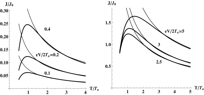
Figure 1: Temperature dependence of drag current. The thin lines, corresponding to the $T^{-0.77}$ dependence are plotted for comparison.

The thin lines correspond to $T^{-0.77}$ law and are given for the comparison. It is clearly seen that our curves can be also approximated by the $T^{-0.77}$ dependence, although the authors of Refs. DVRPRM and DZRKVN regard this dependence as evidence of Tomonaga-Luttinger liquid behaviour of the quantum wires. Indeed, they argued that the increase of the drag with decreasing temperature in a characteristic power-law fashion is in sharp contrast with the prediction of Fermi liquid theories and, therefore, may serve as a signature of the TL behaviour.

The Fermi liquid result (see Fig. 1) can be visualized as follows. At very low temperatures there is Fermi degeneracy and therefore the drag current as a function of temperature goes up. At higher temperatures the degeneracy is lifted while the average electron energy increases with temperature. This results in decrease of the drag current.

For large values of $n$ and $l$ one can be sure of applicability of the Fermi liquid approach. In our opinion, it would be of great importance to investigate on experiment and theory physical conditions (including the reservoir influence), that would bring about transition from the Fermi to Luttinger liquid behavior for small values of $n$ and $l$. This problem seems to be not simple since such an investigation should take into account the influence of number of 1D bands in the quantum wire, the vicinity of reservoirs, the electron-phonon interaction, and, of course, the role of temperature.

We would like to point out some outcomes of our theory. First, the interwire influence can be of importance for the scaled down devices. According to our theory, to minimize an undesired influence of this sort one should avoid the alignment of 1D bands. Second, we note, that as the effect has a maximum as a function of the temperature, this fact also provides some degree of freedom to change such influence. On the other hand, the effect can be used as probe in spectral analysis of nanostructures since it is very sensitive to the alignment of 1D bands. And last, the effect can be important for direct investigation of Coulomb scattering in nanostructures.

References

- (1) Pogrebinskii M. B., Sov. Phys. Semicond. 11, 372, (1977)
- (2) P. J. Price, Physica B, 117, 750 (1983)
- (3) A. G. Rojo, J. Phys.: Condens. Matter, 11, R31, (1999)
- (4) V. L. Gurevich, V. B. Pevzner, and E. W. Fenton, J. Phys.: Condens. Matter 10, 2551, (1998)
- (5) Gurevich V. L. and Muradov M. I. Pis ma v ZhETF 71, 164 (2000) [JETP Letters 71, 111 (2000)]
- (6) P.Debray, P. Vasilopulos, O. Raichev, R. Perrin, M. Rahman and W. C. Mitchel, Physica E, 6, 694, (1999)
- (7) P. Debray, V. Zverev, O. Raichev, R. Klesse, P. Vasilopulos and R. S. Newrock, J. Phys.: Condens. Matter, 13, 3389, (2001)
- (8) P. Debray, V. Gurevich, R. Klesse and R. S. Newrock, Semicond. Sci. Technol., 17, R21, (2002)
- (9) J. Peguiron, C. Bruder, and B. Trauzettel, Phys. Rev. Lett., 99, 086404, (2007)
- (10) F. Stern, Phys. Rev. Lett., 18, 546, (1967)