Structural phase transition of anisotropic particles and formation of orientation-strain glass with addition of impurities

Abstract

Using a modified Lennard-Jones model for anisotropic particles, we present results of molecular dynamics simulation in two dimensions. In one-component systems, we find crystallization, a Berezinskii-Kosterlitz-Thouless phase, and a structural phase transition, as the temperatures is lowered. In the lowest temperature range, the crystal is composed of three martensitic variants on a hexagonal lattice, exhibiting the shape memory effect. With addition of larger spherical particles (impurities), these domains are finely divided, yielding glass with slow time evolution. With increasing the impurity size, the structural or translational disorder is also proliferated.

Certain anisotropic particles such as KCN form a cubic crystal and, at lower temperatures, they undergo an order-disorder phase transition, where the crystal structure changes to a noncubic one. Furthermore, with addition of impurities, the phase ordering often occurs only on small spatial scales, where heterogeneous orientation fluctuations are pinned ori . In such systems softening of the shear modulus is observed, indicating direct coupling between the molecular orientation and the acoustic phonons, and the molecules often have dipolar moments, yielding dielectric anomaly. These systems with frozen disorder have been identified as orientational glass. As a similar example, metallic ferroelectric glass, called relaxor, with frozen polar nanodomains have been studied extensively relax . Recently, a system of off-stoichiometric intermetallic Ti-Ni was shown to be glassy martensite or strain glass, exhibiting the shape-memory effect and the superelasticity Ren . For a one-component system of hard spheroids, Frenkel and Mulder Frenkel1 performed Monte Carlo simulation to find isotropic liquid, nematic liquid, orientationally ordered solid, and orientationally disordered (plastic) solid. Theoretical approaches on strain glass so far have been a phase-field theory with elastic field and a random temperature Saxena and a spin-glass theory with elastic long-range interaction Lookman .

In this Letter, we propose a simple microscopic model exhibiting orientation-martensitic phase transitions and glass behavior. In two dimensions, we suppose elliptic particles interacting via an angle-dependent Lennard-Jones potential, where their positions are ${\mbox{\boldmath$r$}}_{i}$ and their orientation vectors are ${\mbox{\boldmath$n$}}_{i}=(\cos\theta_{i},\sin\theta_{i})$ ($i=1,\cdots,N$). There can be two particle species 1 and 2 with radii $\sigma_{1}$ and $\sigma_{2}$ and numbers $N_{1}$ and $N_{2}$. We set $N=N_{1}+N_{2}=4096$ and change the composition $c=N_{2}/N$. The pair potential $U_{ij}$ between particles $i\in\alpha$ and $j\in\beta$ ($\alpha,\beta=1,2$) is expressed as

$$U_{ij}=4\epsilon\bigg{[}(1+6A_{ij})({\sigma_{\alpha\beta}}/r_{ij})^{12}-({\sigma_{\alpha\beta}}/r_{ij})^{6}\bigg{]}-C_{ij},$$ (1)

where ${\mbox{\boldmath$r$}}_{ij}={\mbox{\boldmath$r$}}_{i}-{\mbox{\boldmath$r$}}_{j}$, $r_{ij}=|{\mbox{\boldmath$r$}}_{ij}|$, $\sigma_{\alpha\beta}=(\sigma_{\alpha}+\sigma_{\beta})/2$, and $\epsilon$ is the characteristic interaction energy. The particle anisotropy is taken into account by the angle factor,

$$A_{ij}=\chi_{\alpha}({\mbox{\boldmath$n$}}_{i}\cdot\hat{\mbox{\boldmath$r$}}_{ij})^{2}+\chi_{\beta}({\mbox{\boldmath$n$}}_{j}\cdot\hat{\mbox{\boldmath$r$}}_{ij})^{2},$$ (2)

where $\hat{\mbox{\boldmath$r$}}_{ij}=|{\mbox{\boldmath$r$}}_{ij}|^{-1}{\mbox{\boldmath$r$}}_{ij}$ represents the direction of ${\mbox{\boldmath$r$}}_{ij}$. We introduce the anisotropy parameters $\chi_{1}$ and $\chi_{2}$ for the two species. We truncate the above potential for $r_{ij}>r_{c}$ with the cut-off being $r_{c}=3\sigma_{1}$. We also set $C_{ij}=U_{ij}$ at $r_{ij}=r_{c}$ to ensure the continuity of the potential at $r_{ij}=r_{c}$, so there remains a weak angle-dependence in $C_{ij}$. Our potential is analogous to the Gay-Berne potential for anisotropic molecules Gay , which has been used to simulate mesophases of liquid crystals, and the Shintani-Tanaka potential with five-fold symmetry yielding frustrated particle configurations Shintani .

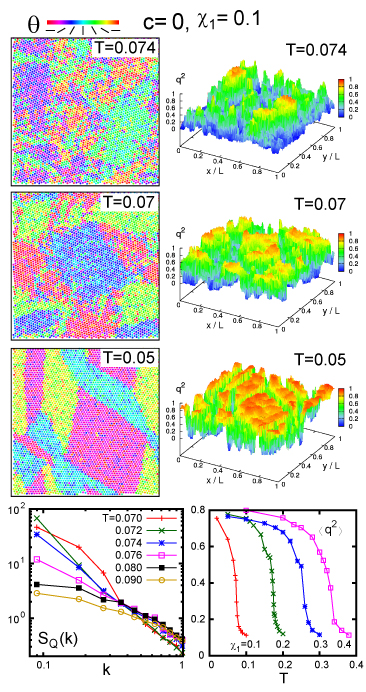
Figure 1: Orientation angle $\theta_{i}$ (left) and order parameter amplitude $q^{2}_{i}$ (right) for $c=0$ and $\chi_{1}=0.1$ at $T=0.074$, $0.07$, and $0.05$ from above. Bottom left: Structure factor $S_{Q}(k)$ of the orientation fluctuations, growing for small $k$ in the range $T_{2}\lesssim T\lesssim T_{1}$. Bottom right: Average amplitude $\langle{q^{2}}\rangle=\sum_{i}q_{i}^{2}/N$ vs $T$ for $\chi_{1}=0.1$, $0.2$, $0.3$, and $0.4$.

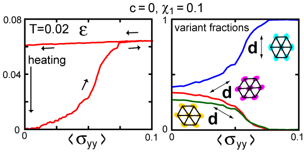
Figure 2: Shape memory effect under uniaxial stretching along the $y$ axis at $T=0.02$ for $c=0$ and $\chi_{1}=0.1$. Left: Strain $\varepsilon$ vs applied stress $\langle{\sigma_{yy}}\rangle$ in units of $\epsilon/\sigma_{1}^{2}$. For $\langle{\sigma_{yy}}\rangle>0.075$, there remains only the variant elongated along the $y$ axis. After this cycle, the residual strain vanishes upon heating to $T=0.1$. Right: Fractions of the three variants during the cycle, which are stretched along the three crystal axes.

The total potential and kinetic energies are $U=\sum_{i<j}U_{ij}$ and $K=\sum_{i}[m|d{\mbox{\boldmath$r$}}_{i}/dt|^{2}+I_{\alpha}|d\theta_{i}/dt|^{2}]/2$, respectively, where the two species have a common mass $m$ and inertia momenta $I_{1}$ and $I_{2}$. The Newton equations of motions are

$${m}\frac{d^{2}}{dt^{2}}{\mbox{\boldmath$r$}}_{i}=-\frac{\partial{U}}{\partial{{\mbox{\boldmath$r$}}_{i}}},\quad{I_{\alpha}}\frac{d^{2}}{dt^{2}}{\theta}_{i}=-\frac{\partial{U}}{\partial{\theta_{i}}}.$$ (3)

Since we treat equilibrium or nearly steady states at a given temperature $T$, we attach a Nos$\acute{\rm e}$-Hoover thermostat nose to all the particles by adding the thermostat terms in Eq.(3). Space, time, and $T$ will be measured in units of $\sigma_{1}$, $\tau_{0}=\sigma_{1}\sqrt{m/\epsilon}$, and $\epsilon/k_{B}$, respectively. In our simulation, we started with a liquid at $T=2$, quenched the system to $T=0.35$ below the melting temperature $T_{m}\sim 1.0$, and annealed it for $9000\tau_{0}$. We then lowered $T$ to a final low temperature.

Assuming that the particles of the second species are spherical and larger, we set $\chi_{2}=0$, $\sigma_{2}/\sigma_{1}=1.2$ or $1.4$, and $c=0,0.1$ or $0.2$. From Eq.(2) the particles of the species 1 have short and long diameters given by $a_{s}=2^{1/6}\sigma_{1}$ and $a_{\ell}=(1+12\chi_{1})^{1/6}a_{s}$, so their molecular area is $S_{1}=\pi a_{s}a_{\ell}/4$ and their inertia momentum is $I_{1}=(a_{\ell}^{2}+a_{s}^{2})m/4$, while $I_{2}=\sigma_{2}^{2}m/2$ and $S_{2}=\pi 2^{-5/3}\sigma_{2}^{2}$. The packing fraction $(N_{1}S_{1}+N_{2}S_{2})/V$ is fixed at $0.95$ and the system length is about $70\sigma_{1}$. For each particle $i$ of the first species, we introduce the orientation tensor ${\stackrel{{\scriptstyle\leftrightarrow}}{{Q}}}_{i}=\{Q_{i\mu\nu}\}$ ($\mu,\nu=x,y$) as

$$\stackrel{{\scriptstyle\leftrightarrow}}{{Q}}_{i} = ({1+N_{\rm b}^{i}})^{-1}({\mbox{\boldmath$n$}}_{i}{\mbox{\boldmath$n$}}_{i}+\sum_{j\in{\rm bonded}}{\mbox{\boldmath$n$}}_{j}{\mbox{\boldmath$n$}}_{j})-\stackrel{{\scriptstyle\leftrightarrow}}{{I}}/2$$ (4)

$$= q_{i}({\mbox{\boldmath$d$}}_{i}{\mbox{\boldmath$d$}}_{i}-\stackrel{{\scriptstyle\leftrightarrow}}{{I}}/2),$$

where $\stackrel{{\scriptstyle\leftrightarrow}}{{I}}$ is the unit tensor and ${\mbox{\boldmath$d$}}_{i}$ is the director with $|{\mbox{\boldmath$d$}}_{i}|=1$. The summation is over the bonded particles $(|{\mbox{\boldmath$r$}}_{ij}|<3\sigma_{1}$) of the first species with $N_{\rm b}^{i}$ being the number of these bonded particles. When a hexagonal lattice is formed, it includes the second nearest neighbor particles. The angle of ${\mbox{\boldmath$d$}}_{i}$ varies more smoothly than $\theta_{i}$. The amplitude $q_{i}$ is given by $q_{i}^{2}=2\sum_{\mu,\nu}Q_{i\mu\nu}^{2}$.

First, we show numerical results in the one-component case ($c=0$) with $\chi_{1}=0.1$ to study the orientation phase transition on a hexagonal lattice. Here we use the periodic boundary condition at fixed volume, but essentially the same results followed at zero pressure. In Fig.1, we show the orientation angle $\theta_{i}$ of all the particles (left) and the order parameter amplitude $q^{2}_{i}$ (right) at $T=0.074,0.07$, and $0.05$. From the angle snapshots we recognize emergence of three variants with lowering $T$ due to the underlying hexagonal lattice. The left bottom panel shows the structure factor $S_{Q}(k)=\langle{|Q_{2{\mbox{\boldmath$k$}}}|^{2}}\rangle$ for $Q_{2{\mbox{\boldmath$k$}}}=\sum_{j}(Q_{jxx}-Q_{jyy})\exp({i{\mbox{\boldmath$k$}}\cdot{\mbox{\boldmath$r$}}_{j}})$, while the right bottom panel displays the average $\langle{q^{2}}\rangle=\sum_{i}q_{i}^{2}/N$ over all the particles for $\chi_{1}=0.1,0.2,0.3$, and 0.4. The orientation order develops gradually in a narrow region $T_{2}<T<T_{1}$, where $T_{2}\sim 0.070$ and $T_{1}\sim 0.076$ for $\chi_{1}=0.1$. The $T_{1}$ and $T_{2}$ increase with increasing $\chi_{1}$. In this temperature window, a Berezinskii-Kosterlitz-Thouless (BKT) phase Jose ; Nelson is realized between the low-temperature martensitic phase and the high-temperature orientationally disordered phase, where the orientation fluctuations are much enhanced at long wavelengths. Though our system size is still small, $S_{Q}(k)$ apparently grows as $k^{\eta-2}$ for $k\lesssim 0.5$, where $\eta$ depends on $T$ (where $\eta\cong 0.05$ at $T=0.074$). We should note that Bates and Frenkel Frenkel2 performed Monte Carlo simulation of two-dimensional rods to find the Kosterlitz-Thouless phase transition.

For $T<T_{2}$, the three variants become distinct with sharp interfaces. The surface tension between the variants is about $0.1\epsilon/\sigma_{1}^{2}$ for $\chi_{1}=0.1$ (and is about $0.2\epsilon/\sigma_{1}^{2}$ for $\chi_{1}=0.2$). In the pattern at $T=0.05$ in Fig.1, the junction angles, at which two or more domain boundaries intersect, are multiples of $\pi/6$. This geometrical constraint stops the domain growth at a characteristic size even without impurities Onukibook . Similar patterns were observed on hexagonal planes in a number of experiments Kitano and were reproduced by phase-field simulation Chen .

In our model, the orientation order induces lattice deformations. As a result, softening of the shear modulus $\mu$ occurs near the transition ori , while the bulk modulus $K$ remains of order $20\epsilon/\sigma_{1}^{2}$. In fact, for $c=0$ and $\chi_{1}=0.1$, we have $\mu\sim 3$ at $T=0.1$, $\mu\sim 1.5$ at $T=0.08$, and $\mu\sim 5$ for $T\lesssim 0.05$ in units of $\epsilon/\sigma_{1}^{2}$. Each variant at low $T$ is composed of isosceles triangles elongated along one of the crystal axes, where side lengths are $1.21\sigma_{1}$ and $1.11\sigma_{1}$ for $\chi_{1}=0.1$ at $T=0.05$ in Fig.1.

In our system, there arises a shape memory effectRen . In Fig.2, we applied a stress $\langle{\sigma_{yy}}\rangle$ along the $y$ axis at $T=0.02$ Rahman , treating the surface along it as a free boundary. Initially, the fractions of the three variants were nearly close to $1/3$ and one variant was elongated along the $y$ axis. For very small $\varepsilon<2\times 10^{-3}$, the system deformed elastically with $\mu\sim 2$. However, for $2\times 10^{-3}<\varepsilon<0.075$, the fraction of the favored variant increased up to unity, while those of the disfavored ones decreased. This inter-variant transformation occurs without defect formation. In the next step $\langle{\sigma_{yy}}\rangle$ was decreased slowly from $0.1\epsilon/\sigma_{1}^{2}$. On this return path, the solid was composed of the favored variant only. At vanishing stress, there remained a remnant strain, but it disappeared upon heating to $T=0.1$ above the transition. Here, we may define the effective shear modulus $\mu_{e}$ by $[\partial\epsilon/\partial\langle{\sigma_{yy}}\rangle]^{-1}=4K\mu_{e}/(K+\mu_{e})\cong 4\mu_{e}$. Then $\mu_{e}\sim 0.1-0.8$ during the inter-variant transformation and $\mu_{e}\sim 5$ on the return path.

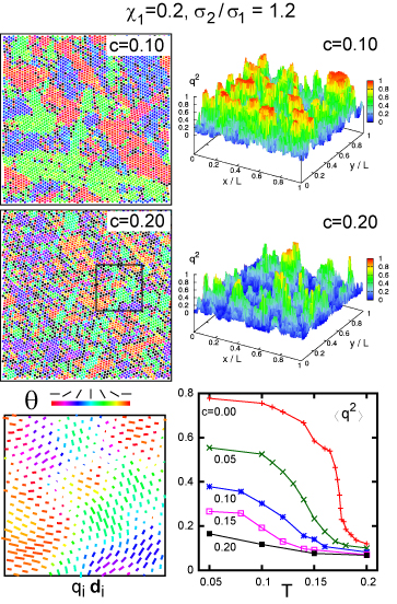
Figure 3: Frozen patterns of angle $\theta_{i}$ (left) and order parameter amplitude $q_{i}$ (right) with impurities for $c=0.1$ and 0.2, where $\chi_{1}=0.2$ at $T=0.05$. Bottom left: Expanded snapshot of $q_{i}{\mbox{\boldmath$d$}}_{i}$ in a box in the upper panel, showing pinned mesoscopic order or strain. Bottom right: $\langle{q^{2}}\rangle$ vs $T$ for various $c$.

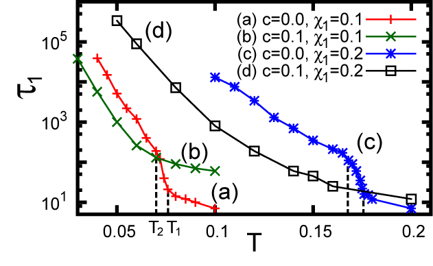
Figure 4: Orientation relaxation time $\tau_{1}$ from the time-correlation function $G_{1}(t)$ for (a) $c=0$ and $\chi_{1}=0.1$, (b) $c=0.1$ and $\chi_{1}=0.1$, (c) $c=0$ and $\chi_{1}=0.2$, and (d) $c=0.1$ and $\chi_{1}=0.2$. It represents the turnover time. For (a) and (c), $\tau_{1}$ grows steeply in the Berezinskii-Kosterlitz-Thouless phase ($T_{2}<T<T_{1}$). For strain glass (b) and (d), this phase is nonexistent and $\tau_{1}$ grows as $T$ is lowered.

Next, in Fig.3, we present examples of strain glass with impurities, where $\sigma_{2}/\sigma_{1}=1.2$ and $\chi_{1}=0.1$. For $c=0.1$ and 0.2, there appeared a few tens of particles with coordination numbers different from six in a single crystal. In our model, the elliptic particles tend to be parallel to the surface of the larger spherical ones, resulting in anchoring of the orientation. We can see that the size of the domains decreases with increasing $c$, where the impurities suppress the development of the orientation order. In addition, the BKT phase disappeared in these examples. We also observed a shape-memory effect even in orientational glass states Ren , where small disfavored domains were replaced by the favored ones upon stretching.

Figure 5: Orientation angle $\theta_{i}$ (left) and six-fold bond orientation angle $\alpha_{i}$ in Eq.(7) (right) in polycrystal for $\sigma_{2}/\sigma_{1}=1.4$ and $c=0.2$, where $\chi_{1}=0.2$ and $T=0.05$.

Now, we discuss the dynamics. Let us consider the time-dependent angle-distribution function,

$$G(t,\varphi)=\sum_{j}\langle{\delta(\theta_{j}(t+t_{0})-\theta_{j}(t_{0})-\varphi)}\rangle/N_{1},$$ (5)

where the average $\langle{\cdots}\rangle$ is taken over the initial time $t_{0}$ and over several runs. We are interested in the first two moments $G_{1}(t)$ and $G_{2}(t)$. For $p=1,2,\cdots$, we define

$$G_{p}(t)=\int_{0}^{2\pi}d\varphi G(t,\varphi)\cos(p\varphi)/2\pi,$$ (6)

which decays from unity on a time scale of $\tau_{p}$. Here, $\tau_{1}$ is the inverse frequency of the turnover motions $\theta_{j}(t)\to\theta_{j}(t)\pm\pi$ at low $T$, while $\tau_{2}$ is the randomization time of $\cos({2\theta_{j}(t)-2\theta_{j}(0)})$. Each turnover motion takes place quickly. We find that $G(t,\varphi)$ exhibits a peak of the form $A(t)\exp[-(\varphi-\pi)^{2}/2\sigma^{2}]/\sqrt{2\pi}\sigma$ for small $\varphi-\pi$ at low $T$, where $\sigma\sim 0.45$. The coefficient $A(t)$ grows linearly as $0.5t/\tau_{1}$ for $t\ll\tau_{1}$ and tends to a constant ($\cong 1/2$) for $t\gg\tau_{1}$. The fitting $G_{1}(t)=\exp[-(t/\tau_{1})^{\beta}]$ fairly holds, where $\beta$ decreases from unity to about 0.5 as $T$ is lowered.

For $c=0$, $\tau_{1}$ increases steeply in the BKT phase and $\tau_{1}^{-1}\propto\exp(-T_{0}/T)$ for $T\lesssim T_{2}$, where (a) $T_{0}\sim 0.40$ at $\chi_{1}=0.1$ and (c) $T_{0}\sim 1.2$ at $\chi_{1}=0.2$ in Fig.4. In addition, $\tau_{1}\sim\tau_{2}$ for $T\gtrsim T_{1}$ but $\tau_{2}/\tau_{1}\gg 1$ for $T\lesssim T_{2}$. In fact, for $\chi_{1}=0.1$, the ratio is about $10^{2}$ at $T=0.07$ and is about $10^{3}$ at $T=0.06$. On the other hand, in glassy states with impurities, the relaxation behavior is more complicated due to the pinning effect, but the turnover motions still occur and $\tau_{2}\gg\tau_{1}$ holds. Figure 4 shows that $\tau_{1}$ for $c=0.1$ is longer in the disordered phase but is shorter in the ordered phase than in the pure system.

For $\sigma_{2}/\sigma_{1}=1.2$ and for $c=0.1$ and 0.2, the crystal structure is little affected by the orientation fluctuations. For a larger size ratio, the structural or positional disorder is more enhanced, eventually resulting in polycrystal and glass Hama . In Fig.5, we realize a polycrystal state for $\sigma_{2}/\sigma_{1}=1.4$, $\chi_{1}=0.2$, and $c=0.2$, where black points represent the impurities. The left panel displays $\theta_{j}$, where there remains noticeable orientation order with $\langle{q^{2}}\rangle=0.2$. The right panel displays the positional sixfold orientation angle $\alpha_{j}$ Nelson ; Hama . Here, for each elliptic particle $j$, we define $\alpha_{j}$ in the range $0\leq\alpha_{j}<\pi/3$ by

$$\sum_{k\in\textrm{\scriptsize{bonded}}}\exp[6i\theta_{jk}]=Z_{j}\exp[{6i\alpha_{j}}],$$ (7)

where $\theta_{jk}$ is the angle of ${\mbox{\boldmath$r$}}_{jk}={\mbox{\boldmath$r$}}_{k}-{\mbox{\boldmath$r$}}_{j}$ with respect to the $x$ axis. We set $|{\mbox{\boldmath$r$}}_{jk}|<1.7\sigma_{1}$ and $Z_{j}>0$.

In summary, we have presented an angle-dependent Lennard-Jones potential to simulate orientation or martensitic transitions. We have added impurities, which pin orientation and strain fluctuations on mesoscopic scales. In future, we should examine the impurity pinning on the glass transition in detail by systematically changing the composition and the size ratio Hama . Competition of the orientational and translational glass behaviors should also be studied. We will shortly report three-dimensional simulation results, where inclusion of the dipolar interaction will enrich the problem.

References

(1)
U. T. Höchli,
K. Knorr, and A. Loidl, Adv. Phys. 39, 405 (1990).
(2)
B. E. Vugmeister and M. D. Glinchuk, Rev. Mod. Phys. 62,
993 (1990).
(3)
S. Sarkar, X. Ren, and K. Otsuka,
Phys. Rev. Lett. 95, 205702 (2005);
Y. Wang, X. Ren, and K. Otsuka,
Phys. Rev. Lett. 97, 225703 (2006).
(4)
D. Frenkel and B. M. Mulder, Mol. Phys. 55, 1171 (1985).
(5) P. Lloveras, T. Castán, M. Porta, A. Planes,
and A. Saxena, Phys. Rev. B 80, 054107 (2009).
(6)
R. Vasseur and T. Lookman,
Phys.Rev.B 81, 094107 (2010).
(7)
J.G. Gay and B.J. Berne, J. Chem. Phys. 74, 3316 (1981);
J.T. Brown, M.P. Allen, E.M. del Rio, and E. Miguel,
Phys.Rev.E, 57, 6685 (1998).
(8)
H. Shintani and
H. Tanaka, Nat. Phys. 2, 200 (2006).
(9)
S. Nosé, Mol. Phys. 52, 255 (1984).
(10) J.V. José, L. P. Kadanoff,
S. Kirkpatrick, and D. R. Nelson, Phys. Rev. B 16,
1217 (1977).
(11) D. R. Nelson and B.I. Halperin,
Phys. Rev. B 19, 2457 (1979).
(12) M. A. Bates and D. Frenkel,
J. Chem. Phys. 112, 10034 (2000).
(13)
A. Onuki, Phase Transition Dynamics (Cambridge University Press, Cambridge, 2002).
(14)
R. Sinclair and J. Dutkiewicz,
Acta Metell. 25, 235 (1977);
Y. Kitano, K. Kifune, and
Y. Komura, J. Phys. (Paris) 49,
C5-201 (1988);
C. Manolikas and S. Amelinckx,
Phys. Stat. Sol. (a) 60, 607 (1980);
ibid. 61, 179 (1980).
(15) Y.H. Wen, Y. Wang, and L.Q. Chen,
Phil. Mag. A. 80, 1967 (2000).
(16)
M. Parrinello and A. Rahman,
J. Appl. Phys., 52, 7182 (1981).
(17) T. Hamanaka and A. Onuki,
Phys. Rev. E 74, 011506 (2006);
H. Shiba and A. Onuki, Phys. Rev. E 81, 051501 (2010).