TRANSPORT OF ENERGETIC ELECTRONS THROUGH THE SOLAR CORONA AND THE INTERPLANETARY SPACE

Abstract

During solar flares fast electron beams generated in the solar corona are non-thermal radio sources in terms of type III bursts. Sometimes they can enter into the interplanetary space, where they can be observed by in-situ measurements as it is done e.g. by the WIND spacecraft. On the other hand, they can be the source of non-thermal X-ray radiation as e.g. observed by RHESSI, if they precipitate toward the dense chromosphere due to bremsstrahlung. Since these energetic electrons are generated in the corona and observed at another site, the study of transport of such electrons in the corona and interplanetary space is of special interest. The transport of electrons is influenced by the global magnetic and electric field as well as local Coulomb collisions with the particles in the background plasma.

1 Introduction

In the solar corona energetic electrons are released e.g. during solar flares and travel along magnetic field lines either toward or away from the Sun (Figure 1). While they propagate through the plasma background they excite Langmuir waves via beam-plasma instability (see e.g. Melrose, (1985)). Partly the energy of Langmuir waves is converted into electromagnetic radiation with a frequency close to the electron plasma frequency $f$

$$f = \sqrt{\frac{e^{2}N_{{\rm e}}}{4\pi^{2}\epsilon_{0}m_{\rm e}}}$$ (1)

and/or its harmonics, where $\epsilon_{0}$, $e$, $m_{\rm e}$ and $N_{\rm e}$ denote the electric constant, the elementary charge, the mass of an electron and the electron number density, respectively.

If those electrons have sufficient energy, and the plasma background is dense enough (as in the case of the solar chromosphere), they can emit non-thermal X-ray radiation via bremsstrahlung (see e.g. Brown, (1972)), which can be detected by spacecrafts as RHESSI. On the other hand electrons moving toward the interplanetary medium up to $1~{}{\rm AU}$ can be observed in-situ by spacecrafts as WIND.

Both methods provide the energies of the electrons either at the X-ray emission site (which is different from the electron acceleration site) or at the current position of the spacecraft in the interplanetary medium. With this information and the model explained in the present paper, it is possible to calculate the altitude of the acceleration site and the kinetic energy that the electrons would have had there.

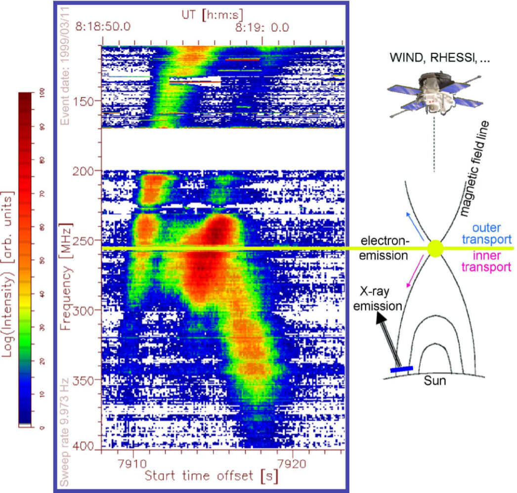
Figure 1: Left: The dynamic spectrum shows type III (and U) radio bursts in the solar corona, which were detected by the AIP spectral polarimeters. (The intensity is colour coded.) Right: The propagation of electrons is schematically illustrated. The fast propagating electrons excite type III radio emissions.

Reference: Önel (2004)

In Section 2 the theoretical model to describe the electron propagation through a given plasma background will be introduced. Next, the plasma background itself is going to be explained in Section 3. Finally in Section 4 some numerical solutions will be presented and in Section 5 the main issues summarised.

2 Model for Electron Transport

The equations of motion for an electron propagating through a given plasma background (the latter explained in Section 3) will be briefly introduced within the current Section, by taking Coulomb collisions, global magnetic and electric fields into account.

Therefore, first the assumptions are explained, which are made to obtain the equations of motion and next the important relations and appearing quantities.

Assumptions

1. Because collisions are easily to treat in the centre of mass system, all calculations are done in this frame of reference. This means, all quantities describe only an effective one-particle system consisting of the electron and the plasma background particles.

2. Within this paper a spherical, heliocentric coordinate system is used consistently.

3. The electric and the nonuniform magnetic fields are treated to be collinear and one dimensional. They are introduced within Section 3 and have only small spatial variations, i.e. the magnetic moment becomes an adiabatic constant of motion.

4. The acceleration by Coulomb collisions is considered to be caused under a small angle scattering approximation, due to the fact, that large angle scattering phenomena are rare in the cases presented within this paper.

Important Relations, Quantities and the Final Equations of Motion

Due to Coulomb collisions, the mean squared scattering angle $\overline{\theta^{2}}_{j}$ will change, according to Jackson (1962), with the time $t$ as

$${\rm d}\overline{\theta^{2}}_{j} \approx \left|\frac{e^{2}q_{j}^{2}N_{j}}{2\pi\epsilon_{0}^{2}\mu_{j}^{2}v_{j,\parallel}^{3}}\ln\left[\sqrt{\frac{\lambda_{\rm D}^{2}+b_{0,\parallel}^{2}}{2b_{0,\parallel}^{2}}}\right]\right|{\rm d}t,$$ (2)

if the electron during its passage through the background plasma is affected by a particle $j$. Here $j$ represents a particle of the plasma background, with charge $q_{j}$ and particle number density $N_{j}$, while $v_{j}$ and $\mu_{j}$ stand for the relative velocity and the effective mass between the background particle and the propagating electron. The other appearing quantities are the Debye length $\lambda_{\rm D}=(\epsilon_{0}k_{\rm{}B}T(N_{\rm{}e}e^{2})^{-1})^{0.5}$, the Boltzmann constant $k_{\rm{}B}$ and the temperature $T$. $b_{0}=e\left|q_{j}\right|(4\pi\epsilon_{0}\mu_{j}v_{j}^{2})^{-1}$ characterises an impact parameter for the effective one particle system, which leads to a deflection of $0.5~{}\pi$ and allows to define $b_{0,\parallel}:=b_{0}\cos^{-2}\left[\Theta_{j}\right]$ by using the pitch-angle $\Theta_{j}=\angle\left[\vec{B},{\vec{v}_{j}}\right]$. Hence the following root-mean-square (RMS) quantity is introduced by definition

$${\rm d}\theta_{{\rm{C}},j} := \sqrt{{\rm d}\overline{\theta^{2}}_{j}}.$$ (3)

The effects caused by the electric field $E$ and the magnetic flux density $B$ to the pitch angle $\Theta_{j}$ are given, as Bai (1982) suggested, by

$$\frac{{\rm{d}}\Theta_{j}}{{\rm d}t} = \frac{\sin[\Theta_{j}]}{v_{j}}\frac{eE}{\mu_{j}}+\frac{v_{j}\sin[\Theta_{j}]}{2B}\frac{{\rm d}B}{{\rm d}r}.$$ (4)

Because of assumption 3 stated on page 3 it is fully sufficient to investigate the scalar quantities only.

If one considers more than one particle species $j$ in the plasma background, as it is described in Section 3, then one has to introduce the following quantities

$${\rm d}\theta_{{\rm{C}},{\rm{total}}} = {\rm d}\theta_{{\rm{C}},{\rm{}e}}+{\rm d}\theta_{{\rm{C}},{\rm{}p}}+{\rm d}\theta_{{\rm{C}},{{\rm{He}}}^{2+}}$$ (5)

$$\Theta_{\rm{total}} = \Theta_{{\rm{}e}}+\Theta_{{\rm{}p}}+\Theta_{{\rm{He}}^{2+}}$$ (6)

$$\mu_{\rm{total}} = \hat{k}_{{\rm{}e}}\,\mu_{{\rm{}e}}+\hat{k}_{{\rm{}p}}\,\mu_{{\rm{}p}}+\hat{k}_{{\rm{He}}^{2+}}\,\mu_{{\rm{He}}^{2+}},$$ (7)

where $\hat{k}_{{\rm{}e}},\hat{k}_{{\rm{}p}}$ and $\hat{k}_{{\rm{He}}^{2+}}$ give the divvies of electrons, protons and $\alpha$-particles inside the plasma background i.e. $j\in\{{\rm{electron}}~{}({\rm{}e}),{\rm{proton}}~{}({\rm{}p}),\alpha{\rm{-particle}}~{}({\rm{He}}^{2+})\}$.

The total velocity is affected both by the electric field and by Coulomb interaction namely as

$$\frac{{\rm{d}}v_{\rm{total}}}{{\rm d}t} = -\frac{eE}{\mu_{\rm{total}}}\cos[\Theta_{\rm{total}}]+\frac{{\rm{d}}v_{\rm{C,total}}}{{\rm d}t}.$$ (8)

Again if one considers the same plasma background as above, one obtains for the Coulomb acceleration, which is the last term of Equation (8) the following expression

$$\frac{{\rm{d}}v_{\rm{C,total}}}{{\rm d}t} := \frac{{\rm{d}}v^{*}_{\rm{}e}}{{\rm d}t}+\frac{{\rm{d}}v^{*}_{\rm{}p}}{{\rm d}t}+\frac{{\rm{d}}v^{*}_{{\rm{He}}^{2+}}}{{\rm d}t},$$ (9)

where each addend is given according to Jackson (1962) by

$$\frac{{\rm{d}}v^{*}_{j}}{{\rm d}t} = -\frac{e^{2}{N_{j}\rm{sign}}\left[v^{*}_{j}\right]}{4\pi\epsilon_{0}^{2}}\left(\frac{q_{j}}{\mu_{j}{v^{*}_{j}}}\right)^{2}\ln\left[\sqrt{\frac{\lambda_{\rm D}^{2}+b_{0}^{2}}{2b_{0}^{2}}}\right].$$ (10)

Hence, Equation 9 shows that the total Coulomb acceleration is given by the sum of the electron, proton and ${\rm{He}}^{2+}$ accelerations. Under the convention that $v_{j}^{*}<0$ for an electron moving toward the Sun and $v_{j}^{*}>0$ for one propagating outward, ${\rm{sign}}\left[v_{j}^{*}\right]$ in Equation (10) makes sure, that the acceleration is in fact a deceleration of the electron velocity. Therefore Equation (10) represents a kind of friction, which forces the electron to stop due to its energy loss per collision. At last, the change of the radial component $r$ of the coordinate of the effective one-particle system’s movement is given by

$$\frac{{\rm{d}}r}{{\rm d}t} = v_{{\rm{total}}}\cos\left[\Theta_{{\rm{total}}}\right]=:v_{{\rm{total}},\parallel}.$$ (11)

If the initial altitude $r_{0}:=r[t_{0}]$, initial velocity $v_{{\rm{total}},0}:=v_{{\rm{total}}}[t_{0}]$ and initial pitch-angle $\Theta_{{\rm{total}},0}:=\Theta_{{\rm{total}}}[t_{0}]$ with the introduced previous equations are given then it is possible to calculate the propagation of an electron away from the acceleration site with the following final equations of motion:

$$r[t+{\rm d}t] = v_{\rm{total}}[t]\cos\left[\Theta_{\rm{total}}[t]\right]{\rm d}t$$ (12)

$$v_{{\rm{total}}}[t+{\rm d}t] = v_{\rm{total}}[t]+\left.\frac{{\rm{d}}v_{\rm{total}}}{{\rm d}t}\right|_{t,\Theta_{\rm{total}}\left[t\right]}{\rm d}t$$ (13)

$$\Theta_{{\rm{total}}}\left[t+{\rm d}t\right] = \Theta_{\rm{total}}\left[t\right]+\left.\left(\frac{{\rm{d}}\Theta_{{\rm{total}}}}{{\rm d}t}+{\mathcal{P}}\frac{{\rm{d}}\theta_{\rm{C,total}}}{{\rm d}t}\right)\right|_{t,\Theta_{\rm{total}}\left[t\right]}{\rm d}t$$ (14)

Here $\mathcal{P}$ denotes the result of a binary dice, whose results $-1$ and $1$ are equally distributed. This is needed to consider the random Coulomb scattering directions. Equation (14) explains the relation between $\Theta_{\rm{total}}$ and $\theta_{\rm{C,total}}$. These presented Equations are sensitive to the models of the plasma background, i.e. the plasma densities, the magnetic fields and the electric fields. The geometry of the electric and the magnetic field has been arranged by assumption 3 on page 3.

Note that those equations allow a so-called backward calculation (${\rm d}t<0$). Therefore this method provides a good possibility for estimating the altitude and the energies of the electrons both at the acceleration site ($t=0=:t_{0}$), if for any $t_{\rm{}f}>t_{0}$ the altitude $r[t_{\rm{}f}]$, the velocity $v_{{\rm{total}}}[t_{\rm{}f}]$ and the pitch-angle $\Theta_{{\rm{total}}}[t_{\rm{}f}]$ are known.

These kind of information (as mentioned in the Section 1) can be obtained e.g. by combining RHESSI and WIND data. Then, one has to assume a standard flare model, which implies that the acceleration site emits the electrons in both directions (in- and outward) simultaneously.

Figure 2: Left: The model of Newkirk (1961), as given by Equation (15), is plotted for several different $\alpha$s (dashed lines) together with the introduced model by Mann et al. (1999) (solid line). It is clearly visible that $r_{\rm S}$ is a function of $\alpha$. Right: The density model according to Mann et al. (1999) is plotted up to a range of $1~{}{\rm AU}\approx{}215~{}R_{\rm Sun}$.

3 Plasma Background

Within this Section the plasma background i.e. the model for the densities, the global magnetic and electric fields are introduced.

3.1 Density Models

The composition of the background plasma is assumed to be fully ionised and containing electrons, protons and $\alpha$-particles: $N_{\rm{}e}=\hat{k}_{{\rm{}e}}N\approx 0.52N$, $N_{\rm{}p}=\hat{k}_{{\rm{}p}}N\approx 0.44N$, and $N_{{\rm He}^{2+}}=\hat{k}_{{\rm He}^{2+}}N\approx 0.04N$, where $N$ denotes the total particle number density, which is the sum of the electron $N_{\rm{}e}$, the proton $N_{\rm{}p}$ and the ${\rm He}^{2+}$ $N_{{\rm He}^{2+}}$ densities. Note that these quantities lead to a mean atomic weight of $\tilde{\mu}=0.6$ as given in Priest (1984).

For the coronal density model, one can use the $\alpha$-fold-Newkirk (1961) model illustrated in Figure 2 and given with the following equation

$$N_{{\rm Newkirk}}[r,\alpha] = 4.2\alpha\hat{k}_{{\rm{}e}}^{-1}\times{}10^{10+4.32~{}R_{\rm Sun}/r}\quad{}{\rm m}^{-3},$$ (15)

while $R_{\rm Sun}\approx 6.958\times 10^{8}~{}{\rm m}$ denotes one solar radius. The $\alpha$ parameter is supposed to be about $1$ in the case of the quite, about $4$ for the active and about $10$ for the super active Sun. Due to the fact, that the Newkirk (1961) model is only valid close to the Sun, an interplanetary density model has to be taken into account additionally. Mann et al. (1999) introduced such a model, which considers the stationary flow of the solar wind, by solving the wind equation of Parker (1981) and the equation of continuity simultaneously

$$\frac{\hat{v}}{\hat{v}_{\rm{}c}^{2}}\frac{{\rm d}\hat{v}}{{\rm d}r} = -\frac{{\rm d}}{{\rm d}r}\big{[}\ln\left[N\right]\big{]}-2\frac{r_{\rm{}c}}{r^{2}}$$ (16)

$$N\hat{v}r^{2} = 1.2\times 10^{34}~{}{\rm Hz},$$ (17)

with $\hat{v}_{\rm{}c}:=(k_{\rm B}T\tilde{\mu}^{-1}m_{\rm{}p}^{-1})^{0.5}$ and $r_{\rm{}c}:=0.5\,GM_{{\rm Sun}}\,\hat{v}_{\rm{}c}^{-2}$. Here $G$ stands for the Newtonian constant of gravitation, $M_{{\rm Sun}}\approx 1.985\times 10^{30}~{}{\rm kg}$ represents the mass of the Sun and $m_{\rm{}p}$ the mass of a proton, while $\hat{v}$ is the velocity of the solar wind. For a temperature of $T=10^{6}~{}{\rm K}$ one obtains $\hat{v}_{\rm{}c}\approx 120~{}{\rm Mm\,s^{-1}}$ and $r_{\rm{}c}\approx 4.2~{}R_{\rm Sun}$ while the numerical solution of the Equations (16) and (17) provide the interplanetary density model of Mann et al. (1999), which is shown in Figure 2.

To combine the presented models of Newkirk (1961) and Mann et al. (1999) one has to introduce $r_{\rm S}$ as the point of intersection between both of them, then

$$N[r,\alpha]=\left\{{N_{{\rm Newkirk}}[r,\alpha]\atop{N_{{\rm Mann}}[r]}}\right. {\rm for} {{1~{}R_{\rm Sun}<r<r_{{\rm S}}}\atop{5~{}{\rm AU}>r\geq{}r_{{\rm S}}}},$$ (18)

with $\alpha=4$ (and $r_{\rm S}[\alpha=4]\approx 1.12~{}R_{\rm Sun}$) yields to the density model, which is used within this paper (see Önel (2004,2005) for more information about this explained density model).

3.2 Global Magnetic Field

In the present paper the coronal magnetic field model $B_{{\rm D\&M}}$ of Dulk & McLean (1978) and the interplanetary magnetic field model $B_{{\rm M\&N}}$ of Marini & Neubauer (1990) by considering Musmann et al. (1977) as well as Parker (1958) are combined as elucidated in Önel (2004).

This yields to a global magnetic field model which is plotted in Figure 3 and described by the following equations:

$$B_{{\rm D\&M}}[r] = \left(\frac{\sqrt[3]{4}\,r}{R_{\rm Sun}}-\sqrt[3]{4}\right)^{-3/2}\times 10^{-4}~{}{\rm T}\quad{\rm for~{}}1.02~{}R_{\rm Sun}\mathrel{\mathchoice{\vbox{\offinterlineskip\halign{\hfil$\displaystyle#$\hfil\cr<\cr\sim\cr}}}{\vbox{\offinterlineskip\halign{\hfil$\textstyle#$\hfil\cr<\cr\sim\cr}}}{\vbox{\offinterlineskip\halign{\hfil$\scriptstyle#$\hfil\cr<\cr\sim\cr}}}{\vbox{\offinterlineskip\halign{\hfil$\scriptscriptstyle#$\hfil\cr<\cr\sim\cr}}}}{}r\mathrel{\mathchoice{\vbox{\offinterlineskip\halign{\hfil$\displaystyle#$\hfil\cr<\cr\sim\cr}}}{\vbox{\offinterlineskip\halign{\hfil$\textstyle#$\hfil\cr<\cr\sim\cr}}}{\vbox{\offinterlineskip\halign{\hfil$\scriptstyle#$\hfil\cr<\cr\sim\cr}}}{\vbox{\offinterlineskip\halign{\hfil$\scriptscriptstyle#$\hfil\cr<\cr\sim\cr}}}}10~{}R_{\rm Sun}$$ (35)

$$B_{{\rm M\&N}}[r] = \sqrt{\frac{7.988~{}{\rm T}^{2}\,{\rm m}^{4}}{r^{4}}+\frac{9.6112\times{}10^{7}~{}{\rm T}^{2}\,{\rm m}^{2.2}}{r^{2.2}}}\quad{\rm for~{}}10~{}R_{\rm Sun}\mathrel{\mathchoice{\vbox{\offinterlineskip\halign{\hfil$\displaystyle#$\hfil\cr<\cr\sim\cr}}}{\vbox{\offinterlineskip\halign{\hfil$\textstyle#$\hfil\cr<\cr\sim\cr}}}{\vbox{\offinterlineskip\halign{\hfil$\scriptstyle#$\hfil\cr<\cr\sim\cr}}}{\vbox{\offinterlineskip\halign{\hfil$\scriptscriptstyle#$\hfil\cr<\cr\sim\cr}}}}{}r\mathrel{\mathchoice{\vbox{\offinterlineskip\halign{\hfil$\displaystyle#$\hfil\cr<\cr\sim\cr}}}{\vbox{\offinterlineskip\halign{\hfil$\textstyle#$\hfil\cr<\cr\sim\cr}}}{\vbox{\offinterlineskip\halign{\hfil$\scriptstyle#$\hfil\cr<\cr\sim\cr}}}{\vbox{\offinterlineskip\halign{\hfil$\scriptscriptstyle#$\hfil\cr<\cr\sim\cr}}}}1{\rm~{}AU}$$ (52)

$$B[r] = \left\{{B_{{\rm D\&M}}[r]}\atop{B_{{\rm M\&N}}[r]}\right.\quad{\rm for~{}}{{1.02~{}R_{\rm Sun}\mathrel{\mathchoice{\vbox{\offinterlineskip\halign{\hfil$\displaystyle#$\hfil\cr<\cr\sim\cr}}}{\vbox{\offinterlineskip\halign{\hfil$\textstyle#$\hfil\cr<\cr\sim\cr}}}{\vbox{\offinterlineskip\halign{\hfil$\scriptstyle#$\hfil\cr<\cr\sim\cr}}}{\vbox{\offinterlineskip\halign{\hfil$\scriptscriptstyle#$\hfil\cr<\cr\sim\cr}}}}r\leq 10~{}R_{\rm Sun}}\atop{10~{}R_{\rm Sun}\leq r\mathrel{\mathchoice{\vbox{\offinterlineskip\halign{\hfil$\displaystyle#$\hfil\cr<\cr\sim\cr}}}{\vbox{\offinterlineskip\halign{\hfil$\textstyle#$\hfil\cr<\cr\sim\cr}}}{\vbox{\offinterlineskip\halign{\hfil$\scriptstyle#$\hfil\cr<\cr\sim\cr}}}{\vbox{\offinterlineskip\halign{\hfil$\scriptscriptstyle#$\hfil\cr<\cr\sim\cr}}}}1{\rm~{}AU}}}$$ (69)

3.3 Global Electric Field

If one considers the small mass of an electron compared to every other ion, then, one can derive the way demonstrated in Önel (2004), a global electric field $E$, shown in Figure 3, from the spherical, hydrodynamical Euler equation for an ideal, isothermal electron fluid, if only the electrostatic force density is taken into account:

$$E[r] = -\frac{k_{\rm B}T}{e}\cdot\frac{{\rm d}}{{\rm d}r}\Bigg{[}\ln\Big{[}N\big{[}r\big{]}\Big{]}\Bigg{]}$$ (70)

Using Equation (70) one can calculate an electrostatic potential difference of $1.8~{}{\rm kV}$ between the photosphere ($r=1~{}R_{\rm Sun}$) and the Earth ($r=1~{}{\rm AU}$) by assuming the introduced density model Equation (18).

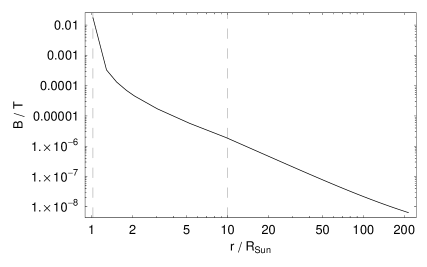
Figure 3: Left: The global magnetic field given by Equation (69) is shown. Right: The global electric field given by Equation (70) is illustrated.

4 Discussions

Within this Section two diagrams (Figure 4), one for the inner and one for the outer transport, will be explained. These diagrams are not related to any particular solar event. Their purpose is to show how those quantities are effected by global magnetic and electric fields, and local Coulomb collisions. Both diagrams in Figure 4 contain an altitude–time $r[t]$, electron plasma frequency (from Equation (1))–time $f[t]$, energy–time $W[t]$ and a pitch-angle–time $\Theta[t]:=\Theta_{\rm{total}}[t]$ evolution for an electron. (Please keep in mind, that due to the chosen centre of mass system those quantities describe only the effective one-particle system electron-plasma background particle.) In addition, the energy amount belonging to the velocity component parallel (drift energy) and perpendicular (Larmor energy) to the magnetic flux density is plotted within the energy–time diagram.

In both diagrams, based on usual our observations of type III burst origins (e.g. Figure 1), an electron at an initial altitude (of approximately $r_{0}\approx 1.127~{}R_{\rm Sun}{}$), which corresponds to an electron plasma frequency of $300~{}{\rm{MHz}}$, with a total initial energy amount of $50~{}{\rm{k}}e{\rm{V}}$, and an initial pitch-angle of $\Theta_{{\rm{total}},0}=0.25~{}\pi$ are assumed. This means, that the initial velocity components parallel and perpendicular to the magnetic flux density are equal, so that at the acceleration site ($t=t_{0}$) the drift and the Larmor energies for the electron are exactly half of the total energy amount.

As it can be seen from Figure 4 the electron moving toward the Sun transfers its drift energy into Larmor energy due to the magnetic (mirror) forces, while it loses energy due to Coulomb collisions. The energy gain caused by the electric forces is insufficient to accelerate the electron, which stops in its radial movement about $0.4~{}{\rm{s}}$ later. The electron moving toward the interplanetary space behaves reversed: It transfers its Larmor energy into drift energy due to the magnetic mirror forces, while it also loses energy due to Coulomb collisions and the electric forces. Due to the decreasing particle density of the atmosphere and its high drift energy, this electron is able to leave the solar atmosphere, with less energy loss. Note, that the transport calculations are done $1\,000$ times for each transport direction. Afterwards all single results for each direction have been averaged arithmetically in the shown Figure 4 to obtain a smooth plot.

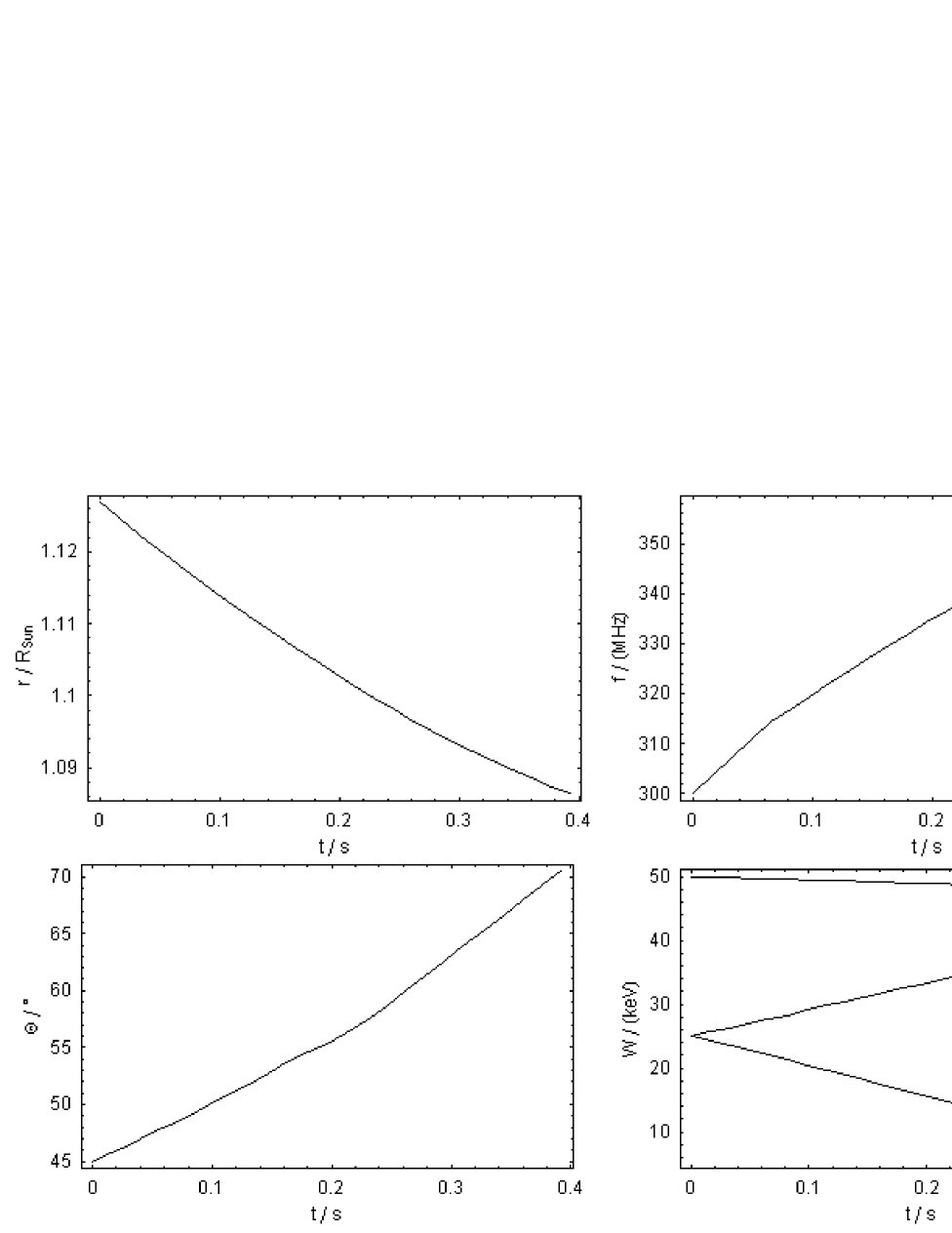
Figure 4: Two examples for the electron transport model introduced in Section 2 are shown. The diagrams are explained and discussed in Section 4.

5 Summary

A 1-dimensional model for the propagation of energetic electrons through a certain plasma background, with known average properties has been introduced.

In case energetic electrons produced e.g. during solar flares can penetrate into the interplanetary space, they can be measured in-situ, e.g. by the WIND spacecraft. In addition, energetic electrons are held responsible for the non-thermal X-ray radiation from the chromosphere, which can be observed by RHESSI spacecraft.

Within this paper we performed a numerical study to characterise how the typical quantities during electron propagation could be affected, by considering average models for the local plasma density, the global electric and the magnetic field.

In our opinion, the main improvement of the deduced model, which easily can be modified to treat proton or ion propagation phenomena, compared with earlier common models of the community (e.g. Brown 1972; Bai 1982) is the innovative way of treating the pitch angle by introducing a binary dice.

Acknowledgements.

We appreciate the permission of the physics department of the Technische Universität Berlin to use their computer facilities for our calculations. Furthermore the authors would also like to express their thanks towards all members of the Solar Radio Group at the AIP, and especially to R. Miteva and J. Magdalenić for the productive discussions.
In lovely memories of the physicist Stephan Joachim Simon (TU–Berlin), who died on $05^{\rm{th}}\mbox{~{}April~{}}2005$ at the age of $25$ years.

References

Bai, T., Transport of energetic electrons in a fully ionized hydrogen plasma, ApJ, 259, 341–349, 1982.

Brown, J. C., The Directivity and Polarisation of Thick Target X-ray Bremsstrahlung from Solar Flares, Solar Phys. 26, 441–459, 1972.

Dulk, G. A., and D. J. McLean, Coronal magnetic fields, Solar Phys., 57, 279–295, 1978.

Jackson, J. D., Classical Electrodynamics, John Wiley & Sons, New York and London, 625–660, 1962.

Newkirk, G. A., The Solar Corona in Active Regions and the Thermal Origin of the Slowly Varying Component of Solar Radio Radiation., ApJ, 133, 983–1013, 1961.

Mann, G., F. Jansen, R. J. MacDowall, M. L. Kaiser, and R. G. Stone, A heliospheric density model and type III radio bursts, A&A, 348, 614–620, 1999.

Mariani, F., and F. M. Neubauer, The Interplanetary Magnetic Field, in Physics of the Inner Heliosphere I: Large Scale Phenomena, edited by R. Schwenn, and E. Marsch, Springer-Verlag, Berlin, Heidelberg, 183–204, 1990.

Melrose, D. B., Plasma emission mechanisms, in Solar Radiophysics: Studies of Emission from the Sun at Metre Wavelengths, edited by D. J. McLean and N. R. Labrum, Camebridge University Press, Camebridge, 177–210, 1985.

Musmann, G., F. M. Neubauer, and E. Lammers, Radial variation of the interplanetary magnetic field between $0.3~{}{\rm{AU}}$ and $1.0~{}{\rm{AU}}$, JGZG, 42, 591–598, 1977.

Önel, H., Einfluss von Coulomb-Stößen auf die Ausbreitung von Elektronen im Flare-Plasma der Sonnenkorona, Diploma Thesis at the Technische Universität Berlin, Center for Astronomy and Astrophysics in collaboration with the Astrophysikalisches Institut Potsdam, Berlin, Germany, 2004.

Önel, H., G. Mann, and E. Sedlmayr, Propagation of Energetic Electrons in the Solar Corona and the Interplanetary Space, in Proceedings of the 11th European Solar Physics Meeting The Dynamic Sun: Challenges For Theory And Observations, 11-16 September 2005 Leuven, Belgium, edited by D. Dansey, S. Poedts, A. DE Groof, and J. Andries, Published by ESA Publications, ESA/ESTEC, Noordwijk, NL, ISBN 92-9092-911-1, ISSN 1609-042X, ESA SP-600 CD-ROM, 2005.

Parker, E. N., Dynamics of the Interplanetary Gas and Magnetic Fields, ApJ, 128, 664–676, 1958.

Parker, E. N., Photospheric flow and stellar winds, ApJ, 251, 266–270, 1981.

Priest, E. R., Solar Magnetohydrodynamics, D. Reidel Publishing Company, Dordrecht, 82–83, 1982.