Backreaction in late-time cosmology
Abstract:
We review the effect of the formation of nonlinear structures on the expansion rate, spatial curvature and light propagation in the universe, focusing on the possibility that it could explain cosmological observations without the introduction of dark energy or modified gravity. We concentrate on explaining the relevant physics and highlighting open questions.
1 Introduction
1.1 The role of structure formation in cosmology
The formation of nonlinear structures from tiny almost Gaussian perturbations by gravitational instability is a central topic in cosmology. Most studies are done either in general relativity (GR) using linear perturbation theory around the locally homogeneous and isotropic Friedmann-Lemaître-Robertson-Walker (FLRW) model or in Newtonian gravity, where extensive numerical computations have been done with N-body simulations, preceded and accompanied by analytical work, to access the nonlinear regime of structure formation. The formation of structures is sensitive to the expansion of the universe, so the observed large-scale structure is a valuable probe of cosmological evolution. There is also another side to the matter: perturbations have a significant effect on the expansion rate once they enter the nonlinear regime. In standard linear theory, the effect vanishes on average by construction. In Newtonian gravity, this turns out to be true also in the non-perturbative regime (see section 2.5). However, this result does not carry over to non-perturbative GR, where the geometry is dynamical. Therefore, there could be a large effect on the average expansion rate, the evolution of spatial curvature and light propagation.
The effect of deviations from exact homogeneity and isotropy on the average expansion is known as backreaction. The effect was first studied in 1962 [2], and an in-depth discussion was given 20 years later by George Ellis [3]. Ellis introduced the term fitting problem to describe the issue of finding a model that best describes the average of the real universe with its complex structures. The problems laid out by Ellis and collaborators did not become mainstream concerns in cosmology at the time, which may partly be due to the complexity of the issues. Another likely reason is that cosmological observations were not precise enough to indicate any tension with a homogeneous and isotropic cosmological model based on ordinary GR with ordinary (visible and dark) matter. As more precise data has revealed that such a model disagrees with observations, it has become topical to study backreaction in more detail to see whether it could account for this failure [4, 5, 6, 7]. We review backreaction in classical GR due to the formation of nonlinear structures at late times, with a focus on the possibility that it could explain this discrepancy. We do not aim to give a historical overview of the literature, but rather try to explain the relevant physics and highlight open questions. There are a number of reviews with comprehensive lists of references [9, 10, 8, 11, 12, 13, 14]. We concentrate on structures that are known to exist and that are expected in the standard structure formation scenario based on usual models of inflation. In particular, we do not discuss models with Gpc-scale structures where, for instance, the observer is located near the centre of a large void [15]. We do not discuss the backreaction of classical or quantum perturbations during inflation or reheating [16]. We also do not cover schemes that introduce some extra structures to GR, which may be needed if the ‘fitting problem’ is to be solved for tensorial objects such as the metric [17].
In section 1 we briefly review some relevant cosmological observations and discuss assumptions underlying the FLRW model. In section 2 we put into perspective the equations that govern the average expansion, explain the meaning of average acceleration and discuss the difference between GR and Newtonian gravity. In section 3 we discuss estimates of backreaction in perturbation theory and in non-perturbative models. In section 4 we consider light propagation and the relation of spatially averaged quantities to observables, as well as observational signatures of backreaction. We conclude in section 5 with a summary.
1.2 Cosmological observations
A linearly perturbed homogeneous and isotropic cosmological model with ordinary matter (i.e. matter with non-negative pressure) and ordinary gravity (based on the four-dimensional Einstein-Hilbert action) can explain all observations of the early universe from Big Bang Nucleosynthesis onwards. The simplest such model, known as the Standard Cold Dark Matter (SCDM) model, is matter-dominated at late times and has flat spatial sections. The SCDM model can also account for late-time observations at the accuracy that had been achieved in the 1980s. However, modern observations have shown that the distance to the last scattering surface at redshift is a factor of to larger than predicted [18, 19] (if the Hubble constant is held fixed and primordial perturbations have a power-law spectrum). Observations of type Ia supernovae and large-scale structure [20, 21, 22] show that this discrepancy occurs at redshifts of order unity, that is, at approximately 10 billion years. Most observations probe distances, and the expansion rate is usually inferred through the use of the FLRW relation between the distance and the expansion rate (see section 4). In the FLRW model, the explanation for longer distances is that the expansion has accelerated, so objects have been pushed further away than expected.
There are few model-independent observations of the expansion rate as a function of redshift, but the Hubble parameter today is relatively well known [19]. By combining with measurements of the matter density we obtain [18, 23]. Combining it with the age of the universe instead [24], we get . In the SCDM model, and , so either way we find that the expansion is faster than expected by a factor ranging from to . This finding supports the interpretation of the distance observations in terms of faster expansion. At the moment, model-independently it is possible to say only that the expansion has decelerated less, not that it would have accelerated [25]. Analysis of large scale structure [26], especially in combination with supernova data [27] can provide strong constraints on the evolution of the Hubble parameter, though these constraints depend on the assumption that the universe is close to FLRW. Currently, we cannot conclude that the expansion would have accelerated without assuming the validity of the FLRW approximation.
Within the FLRW model, the conclusion that the expansion rate has accelerated follows directly from kinematical analysis of distance observations [21]. To obtain acceleration in the FLRW model it is necessary to modify the dynamics either by introducing some exotic form of matter that has negative pressure or by changing the laws of gravitation on cosmological scales. In the simplest such model, the CDM model, constant vacuum energy or, equivalently, a cosmological constant is added. The only difference between the CDM model and the SCDM model is that in the former the expansion rate increases at late times, which is sufficient to bring predictions and observations into agreement (although problems appear to remain with structures on large scales [29, 28, 30, 31, 32]). This point is worth emphasizing: anything that changes the expansion rate and the corresponding distances at late times by the right amount (and that does not modify other things too much) accounts for all of the observed discrepancies, whether of luminosities of supernovae, anisotropies of the cosmic microwave background (CMB), the growth rate of structures or other probes. Notably, all the relevant observations involve integrals over long distances or averages over large scales.
1.3 The hypotheses behind the FLRW model
The common justification for using the FLRW model to describe the universe on average is that the universe appears to be homogeneous and isotropic on large scales. However, we have to distinguish between exact and statistical homogeneity and isotropy. Exact homogeneity and isotropy means that the spatial geometry has a local symmetry: all points and directions are equivalent. (The topological structure may break this symmetry globally.) Statistical homogeneity and isotropy means that if we consider a large domain anywhere in the universe, the mean quantities in the domain do not depend on its location, orientation or size, provided that the domain is larger than the homogeneity scale111Assuming that a homogeneity scale exists, that is, that the mean density and other average quantities converge to a scale-independent value as the volume increases. We make this assumption throughout. In statistical physics, this property is known as spatial homogeneity – not to be confused with the GR property of the same name which is related to local symmetry [29]..
In the usual cosmological treatment, the early universe is assumed to be close to exact homogeneity and isotropy in the sense that the difference between the energy density, expansion rate and other quantities between any two spatial locations is small. Cosmological observations, especially the CMB, provide strong support for this assumption222However, it has not been proven and in principle the effects we discuss could also be relevant in the early universe., and we retain it. Nevertheless, when density perturbations become nonlinear at late times, the universe is no longer locally close to homogeneity and isotropy. However, it remains statistically homogeneous and isotropic on large scales, assuming the initial distribution of perturbations had this property. Statistical homogeneity and isotropy (and a homogeneity scale) are predictions of the simplest inflationary models. We assume that these assumptions hold in the real universe, and that the homogeneity scale is of order 100 Mpc. Whether the existence of a homogeneity scale has been observationally established is a matter of contention [33, 29], and studies of the morphology of structures suggest that such a scale is no smaller than 300 Mpc [34].
Two concepts that are sometimes used to motivate the use of the FLRW metric to describe the universe are the Copernican principle and the cosmological principle. According to the former, our location in the universe is not special, whereas according to the latter all locations in the universe are equivalent. However, the Copernican principle says nothing about possible symmetries of the geometry or the matter distribution. It is possible to have a space that has preferred directions or locations, but where the observer is not in a preferred location. On the other hand, the cosmological principle is a statement about spacetime symmetry, however strictly speaking it does not apply to the real universe because the universe contains structures. If the principle is weakened and interpreted to refer to the distribution of structures, then it is nothing but the statement of statistical homogeneity and isotropy. In modern cosmology, this statement is a prediction of simple models of inflation, rather than a principle, and it is subject to observational tests. Neither the Copernican principle nor the cosmological principle (interpreted to refer to large-scale statistical properties) show that the universe would be described by the FLRW model. In the case of observational tests [33, 29, 35, 36, 37, 38, 39], it is important to distinguish whether they probe statistical homogeneity and isotropy, the FLRW metric or the Copernican principle. (For example, the important check proposed in [35] tests the FLRW metric, not the Copernican principle.)
Put simply, the FLRW model describes universes that are locally homogeneous and isotropic on all scales, not universes that are only statistically homogeneous and isotropic. Because there are large local deviations, the average evolution may be far from the FLRW behavior even above the homogeneity scale. The possibility that the observed change in average quantities from those of the SCDM model at late times is due to the formation of structures may be termed the backreaction conjecture.
2 From the local to the average
2.1 The local expansion rate
We assume that the energy density dominates over pressure, anisotropic stress and energy flux everywhere, in other words, that matter can be considered a pressureless ideal fluid, or dust. This assumption does not hold in the real universe, where deviations from dust evolution are important in regions of large density contrast [40]. However, it seems likely that the effect on average quantities is small, because the fraction of volume in such regions is small [41]. For discussion of non-dust matter, see [42, 43, 44, 45]. In GR, the relation between the matter and the geometry is given by the Einstein equation:
| (1) |
where is the Einstein tensor, is Newton’s constant, is the energy–momentum tensor, is the energy density and is the four-velocity of observers comoving with the dust. The gradient of can be decomposed as
| (2) |
where projects orthogonally to , i.e. onto the dust rest frame. The trace is the volume expansion rate, the traceless symmetric part is the shear tensor and the antisymmetric part is the vorticity tensor (see e.g. [46, 47]). In the FLRW case, the volume expansion rate is , where is the Hubble parameter, and the shear and the vorticity vanish.
The equations can be be decomposed into scalar, vector and tensor parts with respect to the spatial directions orthogonal to . We need only the following scalar parts:
| (3) | |||||
| (4) | |||||
| (5) |
where the dot stands for a derivative with respect to the proper time measured by observers comoving with the dust; and are the shear scalar and the vorticity scalar, respectively. In the irrotational case, is the scalar curvature of the hypersurface which is orthogonal to ; see [48] for the definition of this term in the case of non-vanishing vorticity.
Equation (5) shows simply that the energy density is proportional to the inverse of the volume, in other words that mass is conserved. The Hamiltonian constraint (4) is the local equivalent of the Friedmann equation for an arbitrary dust spacetime, and it relates the expansion rate to the energy density, spatial curvature, shear and vorticity. The Raychaudhuri equation (3) gives the local acceleration. We assume that the fluid is irrotational, i.e. that the vorticity is zero. As with the assumption that the matter is dust, the irrotationality assumption is violated in the real universe, but the violation is not expected to change the overall picture because vorticity is expected to be large only in a small fraction of space. See [43] for the case in which the vorticity is non-zero. Because vorticity contributes positively to the acceleration, setting it to zero gives a lower bound. In this case, the local acceleration is always negative, or at most zero, which simply expresses the fact that gravitation is attractive for matter that satisfies the strong energy condition, which here reduces to .
2.2 The average expansion rate
When discussing averages, the first question concerns the choice of the hypersurface on which the average is taken. We choose the hypersurface orthogonal to , which is also the hypersurface of constant proper time measured by the observers; we discuss this choice in section 4. The spatial average of a scalar quantity is its Riemannian volume integral over a compact domain on the hypersurface, divided by the volume of the domain:
| (6) |
where is the determinant of the metric on the hypersurface of constant proper time , and are Gaussian normal coordinates that are constant along geodesics of the dust flow.
Averaging (3)–(5), we obtain the following well-known set of equations [49]333 These equations are the simplest example of the averaged equations known in the literature as the “Buchert equations”.:
| (7) | |||||
| (8) | |||||
| (9) |
where the kinematical backreaction variable contains the effect of inhomogeneity and anisotropy,
| (10) |
and the scale factor is defined so that the volume of the spatial domain is proportional to ,
| (11) |
where has been normalized to unity at time . Because gives the volume expansion rate, this definition of is equivalent to the definition . We also use the notation .
The integrability conditions (9) assure that the volume expansion law is the integral of the volume acceleration law. Whereas the mass conservation law for dust is sufficient in the homogeneous case, in the inhomogeneous case there is a further equation that dynamically relates the averaged intrinsic and extrinsic curvature invariants. Note that in the presence of inhomogeneities the averaged scalar curvature does not obey a separate conservation law as the density does (unlike in FLRW cosmology): only a combination of the average spatial curvature and the kinematical backreaction variable is conserved [10].
The set of averaged equations (7)–(9) has a slightly different physical interpretation than the FLRW equations due to the different meaning of the scale factor. In the FLRW model, the scale factor is a component of the metric, and indicates how the space evolves locally. (The evolution of any finite volume is of course given by the same scale factor.) In the present context, does not describe local behavior, and it is not part of the metric: it gives only the total volume of the region over which the average is taken.
The average kinematical equations above can be written in a form reminiscent of the FLRW model, with the correction terms included as sources [42]:
| (12) | |||||
| (14) | |||||
where the effective energy density and effective pressure are defined as
| (15) | |||||
| (16) |
respectively. This form of the equations suggests interpreting the new sources due to the curvature inhomogeneities in terms of a minimally coupled scalar field [4, 50, 51], which provides a different language in which to talk about inhomogeneities in geometrical variables. However, the effective sources can have more general behavior than a minimally coupled scalar field. The ‘effective kinetic energy’ is not restricted to be positive-definite, and the effective equation of state can correspondingly evolve from larger than to smaller than .
There has been much discussion about the possible gauge-dependence of the average expansion rate [53, 52, 45, 44, 54]. It is useful to distinguish three different concepts: gauge-dependence, coordinate dependence and dependence on the choice of the averaging hypersurface. Gauge choice refers to the mapping between a fictitious background spacetime and the real spacetime. In the covariant formalism, there is no split into background plus perturbations, so the issue of gauge-dependence does not arise. The averaging procedure expressed in the covariant formalism is also independent of the choice of coordinates. The result does, however, depend on the hypersurface on which the average is taken [53, 52, 45, 54]; note that this is a physical choice, not a matter of mathematical description. We discuss the choice of hypersurface in section 4.
2.3 Physical meaning of average acceleration
If the variance of the expansion rate is large enough compared with the shear and the energy density, then the average expansion rate accelerates according to (7) and (10), even though (3) shows that the local expansion rate decelerates everywhere. This feature is related to the fact that time evolution and averaging do not commute, and it may seem somewhat counterintuitive. However, the explanation is rather simple. Because the universe is inhomogeneous, different regions expand at different rates. Regions with faster expansion rate increase their volume more rapidly, by definition. Therefore the fraction of volume in faster expanding regions rises, so the average expansion rate can rise. This effect is missing in the FLRW model. (Whether the average expansion rate actually does rise depends on how rapidly the fraction of faster regions grows relative to the rate at which their expansion rate decelerates.)
To avoid confusion, it is useful to distinguish three different concepts of acceleration. Local acceleration means that the expansion rate of the local volume element increases. Average acceleration means that the rate of growth of the total volume of the region under consideration increases. Finally, apparent acceleration refers to the situation in which observations (typically distance observations) are analyzed by fitting to a FLRW model and the expansion rate of the fitting model accelerates. In the case of the FLRW universe, these three accelerations coincide due to the high symmetry. As discussed in section 1.2, present observations provide strong support for apparent acceleration, whereas average acceleration has not been established in a model-independent manner. (In models where we are located at the centre of a spherically symmetric inhomogeneity, apparent acceleration typically does not correspond to local acceleration or average acceleration [57, 55, 56].) If backreaction is significant in the real universe, the average expansion has to decelerate less than in the SCDM model, but it is not clear whether it actually needs to accelerate, given that if deviations have a large effect on the average expansion rate, they generally also significantly modify its relation to the distance. We return to this topic in section 4.
2.4 Spatial curvature, entropy and topology
It is possible to understand the backreaction effect in terms of the variance of the expansion rate and the backreaction parameter , or alternatively in terms of the average spatial scalar curvature . The key relation is the integrability condition (9) which relates the backreaction variable and the average spatial curvature. The coupling demonstrates the connection between structures that populate the universe and its spatial geometry: not only does the extrinsic curvature (whose trace gives the expansion rate) change but also the intrinsic curvature evolves during structure formation. In the FLRW case, there are no structures, backreaction vanishes and the spatial curvature term in (9) is conserved individually. In this case the spatial curvature evolves as with the local scale factor .
A non-vanishing backreaction term can lead, due to its coupling to the spatial curvature, to a global gravitational instability of the FLRW model. In other words, it is possible that perturbations of the average spatial curvature and the average expansion rate grow so that averages are driven away from the FLRW behavior, as occurs in some scaling models for the average evolution [58]. In the case of the density distribution, over- and underdense regions add up to a prescribed average density as a result of mass conservation. By contrast, contributions of positively and negatively curved regions to the average spatial curvature do not in general cancel, because there is no isolated conservation law for the spatial curvature [59]. It might be expected that in a universe that becomes dominated by voids the average spatial curvature would evolve to become negative, even if it almost vanishes at early times. Whether the spatial curvature actually evolves in this manner has to be resolved in a realistic model; in the FLRW model, even the possibility of such evolution is absent.
The difference between any given model and the homogeneous and isotropic FLRW model is measurable through the (domain-dependent) Kullback–Leibler distance , an information theoretical relative entropy that arises naturally from the non-commutativity of averaging and time-evolution and is likely to increase in the course of structure formation [60]:
| (17) |
where is the volume of the domain. In the FLRW model the relative entropy is zero, because the distribution is completely unstructured.
Intrinsic curvature is also related to the topology of spatial sections. In a Newtonian description of the evolution of structures on a spatially flat background, there is no spatial curvature and there are six different orientable space forms out of which the three-torus is usually chosen. This corresponds to implementing periodic boundary conditions on deviations from the prescribed background. In GR, the situation is more involved due to intrinsic curvature, and there are an infinite number of possible topological space forms. The situation simplifies for GR in 2+1 dimensions. According to the Gauss-Bonnet theorem, for a closed Riemannian two-space, the volume integral of the spatial curvature is a topological invariant related to the Euler characteristic of the two-dimensional manifold. Therefore, the average spatial curvature always evolves as . Correspondingly, it follows from the -dimensional equivalent of the integrability condition (9) that is always proportional to and cannot lead to acceleration [61, 47]. If the topology were also to fix the average curvature in three dimensions, the dynamics of the average spatial curvature, and hence backreaction, would also be constrained by the topology of space in the real universe. However, in three dimensions the relation between topology and curvature is more involved. This is an ongoing area of investigation and, to a large extent, an open discipline of mathematical physics; there has recently been progress in that field because of results by Perelman (see e.g. [62]).
2.5 Newtonian cosmology
The present framework can also be set up for Newtonian gravity; in fact, the averaged equations were derived first in the Newtonian framework (along with the adaptations to GR) [63]. In Newtonian theory, spatial averaging can be defined for all tensor fields (not only scalars, as in GR) by the Euclidean volume integral, where is an Eulerian domain. The local Raychaudhuri equation (3), which governs the acceleration, is the same in both theories, so the averaged equation (7) is also identical. However, there are important differences. In Newtonian theory we can introduce a diffeomorphism that maps the initial (Lagrangian) positions of fluid elements (labelled by their Lagrangian coordinates ) to Eulerian positions at time , , and the fluid deformation can be measured by the gradient . The volume evolution along the trajectories of a collection of fluid elements of an Eulerian domain is then considered through the volume average, , where the domain is comoving with the collection of fluid elements, is the initial domain and denotes the Jacobian of the coordinate transformation from Eulerian to Lagrangian coordinates and measures the local volume deformation. The fluid geometry, as it is embedded into the Euclidean vector space, is described by the Lagrangian metric with the spatial line element
| (18) |
This metric is flat (i.e. Euclidean), because it can be reduced to the form by the inverse of the transformation . In GR, in contrast, the volume deformation is non-integrable. If we introduce non-exact differential forms, and express them in an exact basis, , the metric coefficients give the Riemannian spatial line element
| (19) |
where the former Lagrangian coordinates are now the local coordinates in the tangent space at a point on the Riemannian manifold, and the transformed volume element is now the Riemannian volume element with . The non-existence of the embedding into a Euclidean vector space, i.e. the non-integrability of the volume deformation, gives rise to intrinsic curvature. The backreaction term is built in the same way in both theories from invariants of the expansion tensor. In the Newtonian theory, can be expressed as a full divergence because of the above integrability property. The divergence can then be transformed to a boundary term via Gauß’ theorem444One consequence is that in the Newtonian theory we can provide a morphological interpretation of backreaction: the backreaction variable can be expressed in terms of three of the four Minkowski functionals [10] (section 3.1.2). These measures were introduced into cosmology by Mecke et al. [64] to statistically assess morphological properties of cosmic structure [34, 65].. In GR, by contrast, does not reduce to a boundary term, which is related to the fact that (in 3+1 or more dimensions) the spatial curvature can have non-trivial evolution.
These differences are crucial for backreaction. When we impose periodic boundary conditions in Euclidean space, the backreaction variable is strictly zero on the periodicity scale (a three-torus has no boundary). This is the construction principle for structure formation models in cosmological simulations. Therefore, there is no global backreaction, and simply describes cosmic variance of the peculiar-velocity gradient in the interior of the structure simulation box555We can still compute the backreaction term in Newtonian simulations on scales below the periodicity scale to determine how the evolution of average quantities on scales smaller than the size of the box is affected by backreaction [66].. This point is interesting in itself, because N-body simulations have been set up without investigating backreaction. If were not a full divergence, the construction of N-body simulations would be inconsistent. Because in Riemannian geometry is in general not a boundary term, current cosmological simulations cannot describe a global backreaction effect. If backreaction is substantial, then current Newtonian simulations (as well as Newtonian analytical studies) are inapplicable in circumstances where deviations of the intrinsic curvature are important.
If backreaction is globally significant (and the universe is statistically homogeneous and isotropic), this is due to non-Newtonian aspects of gravity [63, 49, 67, 68, 9, 10, 61, 59, 54, 69, 70]. It is therefore crucial to understand the relation between Newtonian gravity and GR, which is sometimes called the Newtonian limit of GR. In the above description of fluid deformations in GR the Newtonian limit is obtained if the non-integrable deformation one-forms can be reduced to integrable ones, . This limit automatically implies that the geometry is Euclidean, in particular that the intrinsic curvature and the magnetic part of the Weyl tensor vanish everywhere [71]666There is no need to consider a quasi-Newtonian metric form such as the conformal Newtonian gauge, as is often done, to perform this limit. In the comoving-synchronous setting, we obtain the Lagrangian form of the Newtonian equations [72] in this limit, not the Eulerian form as in the conformal Newtonian gauge.. However, it is not clear to which physical circumstances the above formal limiting process corresponds to.
In cosmology (unlike in the asymptotically flat case) the Newtonian limit is not completely understood. In other words, it is not clear under which physical conditions Newtonian gravity gives a good approximation to GR in an extended system with non-linear deviations. In fact, because the Newtonian limit is singular, it would be more accurate talk about the small-velocity, weak field limit of GR, which is qualitatively different from Newtonian gravity [73, 74, 75, 76, 78, 77, 79, 80, 81, 82, 70]. For example, the Newtonian equations have solutions that are not the limit of any GR solution777In [83] the problem is approached from the other side: assuming a Newtonian cosmological model, what is the perturbed GR model that it approximates? However, the question of interest here is instead the following: given a GR model evolved from realistic initial conditions, is there any Newtonian model that approximates it at late times, and if so, what is it?. Newtonian gravity can thus give a misleading picture of gravitational evolution even in the case of slowly moving sources whose gravitational fields are not strong. An important qualitative difference is that in the Newtonian case there exists a global conserved quantity, the total energy, regardless of whether the system is homogeneous or inhomogeneous (as long as it is isolated, i.e. boundary terms can be neglected). That inhomogeneities cannot change the global average expansion rate in Newtonian cosmology can be understood in terms of this constraint. In GR, in the FLRW case, there is a conserved quantity corresponding to the Newtonian energy term, namely the spatial curvature (multiplied by the square of the scale factor). However, in contrast to the Newtonian theory, this conservation law is only due to the FLRW symmetry. If the universe is anisotropic and/or inhomogeneous, there is in general no conservation law for the spatial curvature. GR in 2+1 dimensions is closer to the Newtonian case in the sense that such a conservation law does exist, as discussed in section 2.4.
On a related topic, let us briefly discuss the behavior of spherically symmetric dust distributions in Newtonian gravity and GR. In GR, Birkhoff’s theorem states that spherically symmetric vacuum solutions are also static or homogeneous or both (the theorem can be generalized to the almost spherically symmetric case [84]), and that the only static solution is the Schwarzschild solution. Birkhoff’s theorem has no relevance when the boundary of the region under consideration is not in vacuum. In the case of dust matter, there are two interesting results. First, both in Newtonian gravity and in GR, the evolution of a spherically symmetric dust region depends only on the distribution of matter inside the region. Second, in the Newtonian case, the average evolution is the same as that of a FLRW dust universe. Both of these two statements are sometimes confused with Birkhoff’s theorem, which is unfortunate especially as the second result does not hold in GR, except when the spatial curvature vanishes or is strongly restricted (see [12], section 7.2). From the backreaction point of view, the Newtonian result follows from the fact that is a boundary term that vanishes for spherical symmetry [66]. In GR, this is not the case, and the average evolution can be different from the FLRW model. Spherically symmetric models have been used to demonstrate accelerating expansion due to backreaction [96].
3 Perturbation theory and non-perturbative models
3.1 Perturbative arguments
It has been argued that backreaction is small because the universe remains close to FLRW in the sense that metric perturbations are small even when the density perturbation becomes nonlinear. It is useful to separate two distinct parts of this argument. The first is that the metric perturbations around a FLRW spacetime are small at all relevant times. The second is that smallness of metric perturbations implies that the average evolution remains close to the FLRW case.
Let us first assume that metric perturbations indeed remain small. From this assumption alone we cannot conclude that backreaction would be small, because the perturbations of the expansion rate (and the distance) depend on first and second derivatives of the metric perturbations, the latter of which become large at the same time as the density perturbations. In other words, perturbations of the spacetime curvature are large. Indeed, in the real universe there are deviations of order unity in the local expansion rate and in the spatial curvature (see [85] for estimates of the spatial curvature in astrophysical systems of different sizes). These are not coordinate artifacts, but rather deviations in physically measurable quantities, and any realistic model has to account for them. The local variation is thus of the same size as the observed average deviation from the SCDM model: the issue is whether their distribution is such that positive and negative deviations cancel on average. This question is related to the absence of a conservation law for the average spatial curvature.
Estimates in first order perturbation theory [86, 87, 5, 7, 88, 53] cannot resolve the issue, because the average of the first order perturbation vanishes, and the contribution of the square of the first order perturbations is not gauge-invariant without the contribution of the intrinsic second order perturbations888The separation between the square of first order perturbations and intrinsic second order perturbations is gauge-dependent [89]..
At second order, the effect on the average expansion rate is small [89]. However, when density perturbations become nonlinear, contributions from higher order terms become as important as the second order terms [68, 54]. Nevertheless, the average expansion rate remains close to the FLRW case if there is a coordinate system in which the following conditions hold: (i) the metric perturbations and their first derivatives are small, (ii) the time derivatives of metric perturbations are at most of the same order as the perturbations multiplied by the background Hubble parameter, (iii) the perturbation of the observer four-velocity is small, and (iv) the difference between the observer four-velocity and the four-velocity that defines the averaging hypersurface is non-relativistic [69]. Essentially, because perturbations of the Christoffel symbols remain small in this coordinate system, the spatial structure remains close to linear theory, even though variations in the spacetime curvature are large. Therefore, large deviations cancel in the average, and such models may be termed ’quasi-Newtonian’, because in Newtonian theory cancellation of deviations in the expansion rate is built in, as discussed above. Under these assumptions, the average spatial curvature and the redshift also remain close to the FLRW behavior. However, deviations do not cancel in all quantities. The shear and the variance of the expansion rate become large at the same time as density perturbations, though their contributions to the expansion rate cancel. The average acceleration also deviates much from the background behaviour [90]. This follows from the commutation rule and the feature that the average expansion rate is close to the background while the variance is large. (The commutation rule is a straightforward consequence of (6).) An important quantity in which deviations do not in general cancel is the luminosity distance. There is a counter-example in which all of the above assumptions are satisfied in a perturbed SCDM model, but the luminosity distance receives large corrections so that it is identical to that of the CDM model with [91].
It is not obvious whether the above assumptions are satisfied in the real universe, namely whether the metric remains close to the same global FLRW background everywhere [11, 69]. For example, under the above assumptions the density (assuming a spatially flat background) is , where is the background Hubble rate, is the background scale factor and is the scalar perturbation of the spatial part of the metric. For a dust background, . If we consider a stabilized region with constant density, has a decaying part and a growing part . In this situation, perturbations of the local metric with respect to a global background eventually become large. However, perturbations becoming large does not imply that the gravitational fields would become strong, but simply that the stabilized region becomes more and more different from the expanding background whose density and curvature decrease. (Once the perturbations become large, their growth could be even faster than indicated by this argument.) However, the situation is complicated by the fact that it would be more appropriate to discuss the evolution in terms of the proper time and the orthogonal spatial coordinates instead of the background time and space coordinates (see also [12], section 7.4.2). Once the second derivatives of the metric become large, the coordinate transformation from one to the other is non-perturbative, and the question of whether backreaction is significant seems to escape the reach of standard perturbation theory. If it could be demonstrated that starting from realistic initial conditions, perturbations and their first derivatives have remained small until today, the backreaction issue would be solved for the average expansion rate and redshift (the luminosity distance would require more work).
An alternative to standard perturbation theory is to employ gradient expansion techniques that allow to go substantially beyond the perturbative regime [68, 92]. One further remedy could be the formulation of perturbation theory in the actually curved space sections by employing nonintegrable deformations in the local tangent space [12, 93]. However, even in such a perturbation framework, a global background has to be specified, an issue that might be overcome by the formulation of perturbation theory around the average distribution rather than the background. A first step towards such a theory is presented in [94].
Constructions in which it is assumed that the metric remains close to the FLRW background are thus severely limited in to what extent it is possible to study backreaction. For example, this is true for the new formalism for averaging and perturbation theory presented in [95], which claims that if metric perturbations around a global background metric remain small, the average evolution can be modified only by a possible radiation-like source term due to the gravitational degrees of freedom. Although the assumption of small perturbations around a global background remains to be justified, [95] presents an example of a formalism for obtaining an average geometry (and not only average scalar quantities).
3.2 Non-perturbative models
In addition to perturbative arguments, backreaction has been studied in toy models and semirealistic models that do not rely on perturbation theory.
3.2.1 Exact toy models
A few toy models have demonstrated how backreaction can lead to accelerating expansion in a dust universe by using the exact spherically symmetric solution [96] or a model with two disjoint regions [9]. Apart from their use as existence proofs, such models can be used to understand qualitative features of average acceleration.
In the real universe, the early distribution of perturbations of the density and the expansion rate is very smooth, with only small local variations. However, as perturbations become nonlinear, regions evolve in distinct ways. In a simplified picture, overdense regions slow down more as their density contrast grows, and eventually they turn around and collapse to form stable structures. Underdense regions become even emptier, and their deceleration decreases. Regions thus become more differentiated and the variance of the expansion rate grows, contributing positively to the volume acceleration, as (7) shows.
In [9] a toy model of this evolution was considered, in which two spherically symmetric regions which are taken to individually evolve according to Newtonian gravity. One of these regions is underdense and the other overdense, so they evolve like dust FLRW universes with negative spatial curvature and positive spatial curvature, respectively. There is one free parameter in the model: the relative size of the regions at some instant of time. This parameter can be chosen such that there is a period of accelerated average expansion. Initially, the evolution is close to the FLRW case. As the slower region starts to deviate significantly from the FLRW evolution, the average expansion rate decreases. However, the underdense region eventually comes to dominate the volume, so the average expansion rate rises. If the underdense region catches up quickly enough, not only can the average expansion rate accelerate, but the average Hubble parameter can rise. In the FLRW model such evolution would require a violation of the null energy condition, i.e. an equation of state more negative than , or an equivalent modification of gravity.
As (8) and (10) show, the volume acceleration is bounded from above by the variance of the expansion rate. The average expansion rate is also bounded from above; estimates in terms of the maximum value of the local expansion rate have been proposed. For irrotational dust, the maximum is achieved in a completely empty constant-curvature region, which implies that [97, 98]. This bound is also expected to hold in realistic models, in which vorticity and deviations from dust behavior are not significant in large fractions of volume [43].
The acceleration is due to the interplay between fast and slow expanding regions. The larger the difference between the fast and slow regions is, the more rapidly the fast regions take over and the larger is the acceleration, which explains why the variance in contributes positively to acceleration. For this reason, a period in which the universe decelerates more than in the SCDM model is conducive to acceleration.
3.2.2 A semirealistic model
In the case when the universe is not everywhere near to a global FLRW background, we cannot write down an exact metric from which to calculate the expansion rate. However, because we are interested only in large-scale averages, rather than the local details of every structure, a statistical description is sufficient. To determine the average expansion rate, we need to know which fraction of the volume of the universe has which expansion rate at a given time. One way to do so is to treat the universe as an ensemble of regions in different stages of expansion or collapse, and to have a model for the evolution of the statistical distribution which is faithful to the physics of structure formation.
The problem is well-defined in the sense that the initial conditions, the matter content and the power spectrum are known. For a Gaussian distribution, all statistical information is contained in the power spectrum, and because structure formation is a deterministic process, all statistical quantities at late times can be traced back to the initial power spectrum. The question is how to find a tractable description of the gravitational processing of the initial density field.
A semirealistic model was constructed in [61, 99]. The starting point is that the universe at early times can be described as a dust-dominated spatially flat FLRW model with linear Gaussian perturbations. The idea is to use the number density of peaks and troughs in the initial density field, smoothed on a given scale, as a measure of the fraction of volume occupied by regions of a given density contrast on that scale. The smoothing scale is fixed by the requirement that the root mean square of the smoothed density contrast, is unity at all times; in other words, the smoothing scale evolves to follow the size of typical structures. The regions are taken to be spherical and to evolve as in Newtonian gravity, so they behave like FLRW universes, as in the two-region toy model. The peak number density is known analytically in terms of the initial power spectrum [100]. The power spectrum depends on two parts, the primordial power spectrum, determined in the early universe by inflation or some other process, and the transfer function , which describes the evolution between the primordial era and today in linear theory. Given an (almost) scale invariant power spectrum and the cold dark matter transfer function, the average expansion rate is fixed.
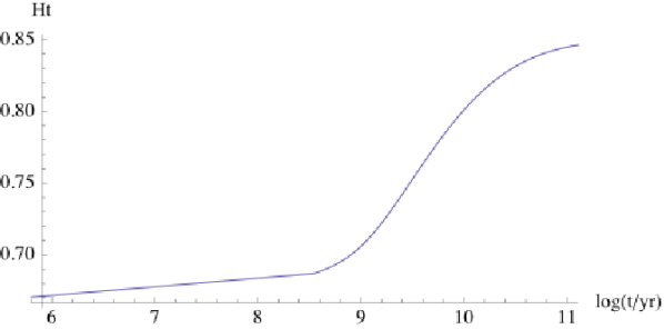
(a)
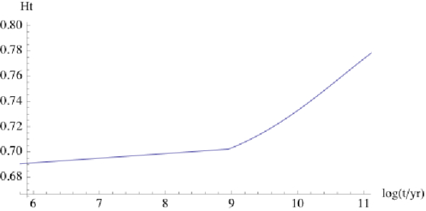
(b)
Figure 1 plots the expansion rate in terms of , showing significant differences from the FLRW behavior at late times. The size of the deviation, to , is of the same order of magnitude as the observed signal, to . More remarkably, the timescale for significant change is 10 billion years, which agrees with observations. The reason for the rise of is that underdense regions take up more and more of the volume. If the universe were completely dominated by totally empty voids, we would have . Because the voids are not completely empty and there are overdense regions, saturates at a value somewhat smaller than unity. (The expansion only decelerates less, the model does not have any acceleration. The absence of acceleration is related to the fact that overdense regions do not appreciably slow down the expansion rate before the underdense regions take over.)
The only scale in the problem is the matter-radiation equality scale Mpc which determines the turnover of the CDM transfer function. Small wavelength perturbations that enter the horizon during the radiation-dominated era are suppressed and perturbations with wavelengths larger than retain (approximately) their original amplitude. The combination of the corresponding matter-radiation equality time yr and the amplitude of the primordial perturbations, , determines when the expansion rate will change significantly. Perturbations with wavelength equal to form non-linear structures when . For a nearly scale-invariant spectrum, this happens when Gyr; after that, there is no scale in the system, so saturates to a constant. Transition begins somewhat earlier at Gyr, as seen in figure 1.
It is interesting that the amplitude of the change in the expansion rate as well as the timescale come out roughly in agreement with observations. However, the model involves uncontrolled approximations, and cannot be trusted beyond an order of magnitude. It is also possible that a more careful statistical treatment would reveal cancellations which significantly change this approximate estimate.
3.2.3 A generic multiscale model
In the same spirit as the previous models, we can consider a general volume partitioning of the universe by introducing a union of disjoint overdense regions and a union of disjoint underdense regions , both of which make up the total region , which is considered to contain the homogeneity scale. The averaged equations can be split accordingly to obtain for the kinematical backreaction [59] the result
| (20) |
where denotes the volume fraction of the overdense regions compared with the volume of the region . In a Gaussian random field this fraction would be and it would gradually drop in a typical structure formation scenario that clumps matter into small volumes and that features voids that gradually dominate the volume in the course of structure formation, see figure 2. A similar construction has been used in the so-called timescape cosmology proposed by Wiltshire [101].
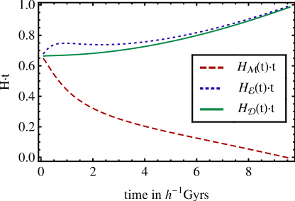
If we ignore, for the sake of simplicity, the individual backreaction terms on the partitioned domains (as in the models discussed above), the total backreaction features a positive-definite term due to the variance of the different expansion rates of over- and underdense regions. This term can lead to acceleration in the volume expansion rate of the domain [102]. Refining the multiscale model by including non-zero individual backreaction terms, for example by an extrapolation of the leading perturbative mode in second-order perturbation theory [103], which also corresponds to the leading order in a Newtonian non-perturbative model (i.e. where the backreaction terms decay in proportion to ) [66], we can even produce a cosmological constant behavior of the scale factor over the homogeneity scale (see figure 3 in [102]). Such behavior can only be transient, however, and the acceleration is expected to be followed by a phase of deceleration.
4 Light propagation
4.1 Connection between the expansion rate and observables
A key question is how the spatial averages discussed thus far are related to observations. This issue is tied to the averages’ dependence on the choice of the hypersurface of averaging. Almost all cosmological observations are made along the lightcone, as they measure the redshift, the angular diameter distance (or equivalently the luminosity distance) and other quantities related to bundles of light rays. In a general spacetime, these quantities are not determined solely by expansion, and certainly not by the average expansion rate along spacelike slices. However, in a statistically homogeneous and isotropic universe in which the distribution evolves slowly, the average expansion rate may determine the leading behavior of the redshift and the distance over large scales [104, 43, 56]. Consideration of the observables also identifies the relevant hypersurface of averaging. In a general dust spacetime, the redshift is given by
| (21) |
where is defined by , and is the spatial direction of the null geodesic. The direction changes slowly for typical light rays [43], whereas the dust shear is correlated with the shape and orientation of structures and changes on the length scale of those structures. If there are no preferred directions, so structures on large scales are oriented in all directions equally, should contribute via its trace, which is zero. Therefore, the integral over should vanish up to statistical fluctuations and corrections from correlations between and and the evolution of the distribution. We can split the local expansion rate as , where is the local deviation from the average, and similarly argue that the integral of is suppressed relative to the contribution of the average expansion rate. The change in the distribution also has to be slow compared with the time it takes for a light ray to pass through a homogeneity scale sized region. If the homogeneity scale today is of the order Mpc, then the crossing time is indeed much smaller than the time scale for the change in the distribution, which is given by the Hubble scale Mpc. In the early universe, structure formation was less advanced, so the homogeneity scale relative to the Hubble scale is even smaller further down the null geodesic.
Here the choice of hypersurface comes into play. The relevant hypersurface is the one in which variations around the mean cancel, in other words the hypersurface of statistical homogeneity and isotropy. Because the evolution of structures is governed by the proper time, one can argue that this hypersurface is close to the hypersurface of constant proper time [9, 61, 104]. However, the two hypersurfaces are not exactly the same, and in the realistic case when the observer four-velocity is not irrotational, the hypersurface of constant proper time is not orthogonal to the observer four-velocity. The details are thus more complicated, but non-relativistic changes in the four-velocity field that defines the hypersurface of averaging lead only to small changes in the average expansion rate, as long as the distribution is statistically homogeneous and isotropic and the averaging scale is at least as large as the homogeneity scale [43]. However, a one-dimensional sample may converge to homogeneity significantly slower than a three-dimensional one [105].
These cancellations also explain why the large variance required for significant backreaction does not necessarily lead to large deviations in the observed CMB temperature (which is given simply by the redshift of the CMB photons). It is sometimes claimed that if all observers measure a nearly isotropic CMB sky, then the universe is nearly FLRW [11]. However, this is not true. Making statements about the geometry also requires assumptions about the spatial derivatives of the CMB temperature field, and these assumptions are not satisfied in the real universe [61, 104, 106]. Observation of a nearly isotropic CMB sky does not imply that the universe is close to FLRW.
Given that , we obtain , the same relation between expansion and redshift as in the FLRW case. This result depends on the fact that the shear and the expansion rate enter linearly into the integral (21) along the null geodesic. In contrast, the shear and the expansion rate enter quadratically into the equations of motion (3)–(5) for the geometry, so variations do not cancel in the average; instead we have the generally non-zero backreaction variable .
For the angular diameter distance, similar qualitative arguments give [104]
| (22) |
where is the dominant part of the angular diameter distance with corrections to the mean dropped, and similarly for the redshift: . (It is not entirely clear that the angular deviation of the distance must necessarily be small [90].)
From the conservation of mass (9), it follows that . The distance is therefore determined entirely by the average expansion rate and the normalization of the density today, namely . For a FLRW model with general matter content, in (22) would be replaced by . Therefore, the equation for the mean angular diameter distance in terms of in a statistically homogeneous and isotropic dust universe (with a slowly evolving distribution) is the same as in the FLRW CDM model. If backreaction were to produce exactly the same expansion history as the CDM model, the distance-redshift relation would therefore also be identical. This is true even though the spatial curvature would be large, because the spatial curvature affects the distance differently than in the FLRW case.
However, backreaction is not expected to produce an expansion history identical to the CDM model: if the expansion accelerates strongly, the acceleration may be preceded by extra deceleration, and the acceleration cannot be eternal (unless the rate of acceleration goes asymptotically to zero sufficiently rapidly). Therefore the backreaction distance-redshift relation also differs from the CDM model, although it is shifted towards CDM compared with a FLRW model with the same expansion history as the backreaction model. The reason is that in any FLRW model apart from CDM, the equation for is modified not only by the mapping between the affine parameter and the redshift (as described by ), but also by the change of the source term , whereas in the backreaction case only the mapping between the affine parameter and the redshift (i.e. ) changes. This feature could explain why distance observations prefer a value close to for the effective equation of state.
Above, we assume that light is passing through a continuous distribution of matter. However, it is not clear whether such an assumption is valid in the real universe, in which matter is clumped on various scales, and it may be that a typical light ray travels in vacuum without crossing any structures. This issue remains to be completely understood [107, 108, 43]; for references on the effect of clumpiness on light propagation, see [104, 108].
A related problem is that light propagation is usually considered in the geometrical optics approximation, with infinitesimal light bundles. However, light wave fronts have a finite extent, which is especially important if the matter distribution is discrete on the relevant scales. Surface averaging of light fronts and its relation to distances should thus be considered. A covariant formalism for averaging on different slices of the past light cone was recently introduced [109]. However, because we observe both the redshift and the angular position of sources, the relevant issue is cancellations along the null geodesic, as discussed above.
4.2 Observational signatures of backreaction
In the FLRW model, there exists a definite relation between and , which can be used as a general test of FLRW models [35]. If the distance and the expansion rate are measured independently [25, 26, 27], we can check whether they satisfy the FLRW relation. If they do not, the observations cannot be explained in terms of any four-dimensional FLRW model. Because the FLRW relationship between and depends on the spatial curvature, a test of the relation can be viewed as a test of whether the spatial curvature is proportional to . If backreaction is significant, the spatial curvature divided by is non-constant for some redshift range. This holds independently of the presence of dark energy or modified gravity, because light propagation directly depends on the geometry of spacetime, regardless of the equations of motion that determine it. The consequences of a different curvature evolution have been analyzed in [110, 102].
The backreaction conjecture that the change in the average expansion rate at small redshift is due to structure formation can be tested without a prediction for the change in the expansion rate, simply by checking whether the measured and satisfy (22). This relation, which violates the FLRW consistency condition between expansion and distance, is a unique prediction of backreaction that distinguishes it from the FLRW model. However, the derivation of the relation should be done more rigorously, and the expected magnitude and shape of the violation are not known.
The redshift, as well as null geodesic shear and deflection [43], should be studied in more detail. In particular, it would be interesting to quantitatively check that light propagation in a statistically homogeneous and isotropic space with a slowly evolving distribution of small structures can be described in terms of the average expansion rate, and to characterize the corrections [61, 104, 43]. The small-scale pattern of the CMB depends only on the angular diameter distance [18], but the effects on large angular scales remain to be determined. Extending weak lensing analysis to the case in which the geometry is not nearly FLRW is also needed for comparison with present and upcoming data.
5 Conclusions
We discuss the backreaction conjecture, namely the possibility that structure formation changes the average expansion rate, spatial curvature and light propagation, thereby eliminating the need for dark energy or modified gravity. The change in the average properties due to structure formation is present in reality but is not taken into account either in the FLRW model and its linear perturbations or Newtonian non-linear models.
The basic mechanism of backreaction is simple and can be demonstrated in toy models: because the universe is inhomogeneous, different regions expand at different rates, so the fraction of volume in faster expanding regions can grow, and the average expansion rate can rise. Structure formation has a preferred time of 10 billion years, which agrees with the observed timescale for the change in the expansion rate, and the amplitude of the change can also be understood from simple considerations. However, the effect has not been quantified in a fully realistic model.
Various things remain to be done before robust quantitative conclusions can be drawn. If backreaction is significant, it cannot be understood simply as a change in the FLRW background model. To analyze signals such as baryon acoustic oscillations and other features in the distribution of large structure, we must develop perturbation theory around a non-FLRW background, where the mean is the average of deviations that have a large amplitude, but a small coherence length.
The treatment of light propagation also needs to be made more rigorous and extended both to cover phenomena such as weak lensing in detail and to include effects due to the discreteness of matter. The deviation of the relation between distance and the expansion rate from the FLRW case is an important prediction, which can be tested without a calculation of the average expansion rate. However, the goal should be to derive the change in the average expansion rate with quantified errors. In addition to statistical models, one way to address the question could be to generalize N-body simulations to include the relevant relativistic degrees of freedom.
The backreaction conjecture is conservative in the sense that it does not involve new fundamental physics, only neglected effects in non-linear GR. Before the effect of structure formation on the average expansion rate is reliably quantified, we will not know whether dark energy or modified gravity is needed. It is plausible that backreaction can explain all of the observations, and even if the large-scale average properties of the universe turn out to be close to the FLRW case, the corrections may nevertheless be quantitatively important.
Acknowledgments.
The work of TB was conducted within the “Lyon Institute of Origins” under grant ANR-10-LABX-66.References
- [1]
- [2] M.F. Shirokov and I.Z. Fisher, Isotropic Space with Discrete Gravitational-Field Sources. On the Theory of a Nonhomogeneous Universe, Astronomicheskii Zhurnal 39 (1962) 899, Reprinted in Sov. Astron. J. 6 (1963) 699, Reprinted in Gen. Rel. Grav. 30 (1998) 1411
-
[3]
G.F.R. Ellis,
Relativistic cosmology: its nature, aims and problems, 1984
The invited papers of the 10th international conference on general relativity and gravitation
p 215
G.F.R. Ellis and W. Stoeger, The ’fitting problem’ in cosmology, Class. Quant. Grav. 4 (1987) 1697 - [4] T. Buchert, On average properties of inhomogeneous cosmologies, 2000, Proc. 9th JGRG conference, ed. Y. Eriguchi et al., p 306 [arXiv:gr-qc/0001056]
- [5] C. Wetterich, Can Structure Formation Influence the Cosmological Evolution?, Phys. Rev. D67 (2003) 043513 [arXiv:astro-ph/0111166]
- [6] D.J. Schwarz, Accelerated expansion without dark energy [arXiv:astro-ph/0209584]
-
[7]
S. Räsänen,
Dark energy from backreaction,
JCAP02(2004)003
[arXiv:astro-ph/0311257]
S. Räsänen, Backreaction of linear perturbations and dark energy [arXiv:astro-ph/0407317] - [8] G.F.R. Ellis and T. Buchert, The universe seen at different scales, Phys. Lett. A347 (2005) 38 [arXiv:gr-qc/0506106]
- [9] S. Räsänen, Accelerated expansion from structure formation, JCAP11(2006)003 [arXiv:astro-ph/0607626]
- [10] T. Buchert, Dark energy from structure – a status report, Gen. Rel. Grav. 40 (2008) 467 (2008) [arXiv:0707.2153 [gr-qc]]
- [11] G.F.R. Ellis, Inhomogeneity effects in Cosmology, Class. Quant. Grav. 28 (2011) 164001 [arXiv:1103.2335 [astro-ph.CO]]
- [12] T. Buchert, Toward physical cosmology: focus on inhomogeneous geometry and its non-perturbative effects, Class. Quant. Grav. 28 (2011) 164007 [arXiv:1103.2016 [gr-qc]]
- [13] S. Räsänen, Backreaction: directions of progress, Class. Quant. Grav. 28 (2011) 164008 [arXiv:1102.0408 [astro-ph.CO]]
- [14] C. Clarkson, G.F.R. Ellis, J. Larena and O. Umeh, Does the growth of structure affect our dynamical models of the Universe? The averaging, backreaction, and fitting problems in cosmology, Rep. Prog. Phys. 74 (2011) 112901 [arXiv:1109.2314 [astro-ph.CO]]
-
[15]
K. Enqvist,
Lemaitre-Tolman-Bondi model and accelerating expansion,
Gen. Rel. Grav. 40 (2008) 451
[arXiv:0709.2044] [astro-ph]
K. Bolejko, M.-N. Célérier and A. Krasiński, Inhomogenous cosmological models: exact solutions and their applications, Class. Quant. Grav. 28 (2011) 164002 [arXiv:1102.1449 [astro-ph.CO]]
V. Marra and A. Notari, Observational constraints on inhomogeneous cosmological models without dark energy, Class. Quant. Grav. 28 (2011) 164004 [arXiv:1102.1015 [astro-ph.CO]] -
[16]
N.C. Tsamis and R.P. Woodard,
Quantum Gravity Slows Inflation,
Nucl. Phys. B474 (1996) 235
[arXiv:hep-ph/9602315]
N.C. Tsamis and R.P. Woodard, The Quantum Gravitational Back-Reaction on Inflation, Annals Phys. 253 (1997) 1 [arXiv:hep-ph/9602316]
L.R. Abramo, N.C. Tsamis and R.P. Woodard, Cosmological Density Perturbations From A Quantum Gravitational Model Of Inflation, Fortsch. Phys. 47 (1999) 389 [arXiv:astro-ph/9803172]
N.C. Tsamis and R.P. Woodard, A Gravitational Mechanism for Cosmological Screening, Int. J. Mod. Phys. D20 (2011) 2847 [arXiv:1103.5134 [gr-qc]]
V.F. Mukhanov, L.R.W. Abramo and R.H. Brandenberger, On the Back reaction problem for gravitational perturbations, Phys. Rev. Lett. 78 (1997) 1624 [arXiv:gr-qc/9609026]
L.R.W. Abramo, R.H. Brandenberger and V.F. Mukhanov, The Energy-momentum tensor for cosmological perturbations, Phys. Rev. D56 (1997) 3248 [arXiv:gr-qc/9704037] -
[17]
M. Carfora and K. Piotrkowska,
Renormalization group approach to relativistic cosmology,
Phys. Rev. D52 (1995) 4393
[arXiv:gr-qc/9502021]
R.M. Zalaletdinov, Averaging problem in general relativity, Macroscopic Gravity and using Einstein’s equations in cosmology, Bull. Astron. Soc. India 25 (1997) 401 [arXiv:gr-qc/9703016]
A. Paranjape and T.P. Singh, Explicit cosmological coarse graining via spatial averaging, Gen. Rel. Grav. 40 (2008) 139 [arXiv:astro-ph/0609481]
T. Buchert and M. Carfora, Regional averaging and scaling in relativistic cosmology, Class. Quant. Grav. 19 (2002) 6109 [arXiv:gr-qc/0210037]
T. Buchert and M. Carfora, Cosmological parameters are ‘dressed’, Phys. Rev. Lett. 90 (2003) 031101 [arXiv:gr-qc/0210045] - [18] M. Vonlanthen, S. Räsänen and R. Durrer, Model-independent cosmological constraints from the CMB, JCAP08(2010)023 [arXiv:1003.0810 [astro-ph.CO]]
-
[19]
N. Jackson,
The Hubble Constant,
Living Reviews in Relativity 10 (2007) 4
[0709.3924 [astro-ph]]
G.A. Tammann, A. Sandage and B. Reindl, The expansion field: The value of , Astron. & Astrophys. 15 (2008) 289 [arXiv:0806.3018 [astro-ph]]
A.G. Riess et al., A Redetermination of the Hubble Constant with the Hubble Space Telescope from a Differential Distance Ladder, Astrophys. J. 699 (2009) 539 [arXiv:0905.0695 [astro-ph.CO]]
A.G. Riess et al., A 3% Solution: Determination of the Hubble Constant with the Hubble Space Telescope and Wide Field Camera 3, Astrophys. J. 730 (2011) 119 [arXiv:1103.2976 [astro-ph.CO]] -
[20]
R.J. Foley et al.,
Spectroscopy of high–redshift supernovae from the Essence Project: the first four years,
Astron. J. 137 (2009) 3731
[arXiv:0811.4424 [astro-ph]]
M. Hicken et al., Improved dark energy constraints from ~100 new CfA supernovae Type Ia light curves, Astrophys. J. 700 (2009) 1097 [arXiv:0901.4804 [astro-ph.CO]]
R. Kessler et al., First-year Sloan Digital Sky Survey-II (SDSS-II) Supernova Results: Hubble Diagram and Cosmological Parameters, Astrophys. J. Suppl. 185 (2009) 32 [arXiv:0908.4274 [astro-ph.CO]]
R. Amanullah et al., Spectra and Light Curves of Six Type Ia Supernovae at 0.511 z 1.12 and the Union2 Compilation, Astrophys. J. 716 (2010) 712 [arXiv:1004.1711 [astro-ph.CO]] -
[21]
C. Shapiro and M.S. Turner,
What Do We Really Know About Cosmic Acceleration?,
Astrophys. J. 649 (2006) 563
[arXiv:astro-ph/0512586]
Y. Gong and A. Wang, Observational constraints on the acceleration of the Universe, Phys. Rev. D73 (2006) 083506 [arXiv:astro-ph/0601453]
Ø. Elgarøy and T. Multamäki, Bayesian analysis of Friedmannless cosmologies, JCAP09(2006)002 [arXiv:astro-ph/0603053]
C. Cattoën and M. Visser, Cosmography: Extracting the Hubble series from the supernova data [arXiv:gr-qc/0703122]
M. Visser and C. Cattoën, Cosmographic analysis of dark energy, Dark matter in astrophysics and particle physics: proceedings of the 7th International Heidelberg Conference on Dark 2009, ed. H.V. Klapdor-Kleingrothaus and I.V. Krivosheina, World Scientific Publishing, p 287 [arXiv:0906.5407 [gr-qc]]
M. Seikel and D.J. Schwarz, How strong is the evidence for accelerated expansion?, JCAP02(2008)007 [arXiv:0711.3180 [astro-ph]]
M. Seikel and D.J. Schwarz, Model- and calibration-independent test of cosmic acceleration, JCAP02(2009)024 [arXiv:0810.4484 [astro-ph]]
E. Mörtsell and C. Clarkson, Model independent constraints on the cosmological expansion rate, JCAP01(2009)044 [arXiv:0811.0981 [astro-ph]]
A.C.C. Guimarães, J.V. Cunha and J.A.S. Lima, Bayesian Analysis and Constraints on Kinematic Models from Union SNIa, JCAP10(2009)010 [arXiv:0904.3550 [astro-ph.CO]]
M.V. John, Delineating cosmic expansion histories with supernova data [arXiv:0907.1988 [astro-ph.CO]] - [22] W.J. Percival et al., Baryon Acoustic Oscillations in the Sloan Digital Sky Survey Data Release 7 Galaxy Sample, Mon. Not. Roy. Astron. Soc. 401 (2010) 2148 [arXiv:0907.1660 [astro-ph.CO]]
- [23] P.J.E. Peebles, Probing General Relativity on the Scales of Cosmology [arXiv:astro-ph/0410284]
- [24] L.M. Krauss and B. Chaboyer, Age Estimates of Globular Clusters in the Milky Way: Constraints on Cosmology, Science 299 (2003) 65
-
[25]
R. Jimenez and A. Loeb,
Constraining Cosmological Parameters Based on Relative Galaxy Ages,
Astrophys. J. 573 (2002) 37
[arXiv:astro-ph/0106145]
J. Simon, L. Verde and R. Jimenez, Constraints on the redshift dependence of the dark energy potential, Phys. Rev. D71 (2005) 123001 [arXiv:astro-ph/0412269]
D. Stern, R. Jimenez, L. Verde, M. Kamionkowski and S.A. Stanford, Cosmic Chronometers: Constraining the Equation of State of dark energy. I: H(z) Measurements, JCAP02(2010)008 [arXiv:0907.3149 [astro-ph.CO]]
M. Moresco, R. Jimenez, A. Cimatti and L. Pozzetti, Constraining the expansion rate of the Universe using low-redshift ellipticals as cosmic chronometers, JCAP03(2011)045 [arXiv:1010.0831 [astro-ph.CO]] -
[26]
E. Gaztañaga, A. Cabré and L. Hui,
Clustering of Luminous Red Galaxies IV: Baryon Acoustic Peak in the Line-of-Sight Direction and a Direct Measurement of H(z),
Mon. Not. Roy. Astron. Soc. 399 (2009) 1663
[arXiv:0807.3551 [astro-ph]]
E. Gaztañaga, R. Miquel and E. Sánchez, First Cosmological Constraints on dark energy from the Radial Baryon Acoustic Scale, Phys. Rev. Lett. 103 (2009) 091302 [arXiv:0808.1921 [astro-ph]]
J. Miralda-Escude, Comment on the claimed radial BAO detection by Gaztanaga et al. [arXiv:0901.1219 [astro-ph]]
E.A. Kazin, M.R. Blanton, R. Scoccimarro, C.K. McBride and A.A. Berlind, Regarding the Line-of-Sight Baryonic Acoustic Feature in the Sloan Digital Sky Survey and Baryon Oscillation Spectroscopic Survey Luminous Red Galaxy Samples, Astrophys. J. 719 (2010) 1032 [arXiv:1004.2244 [astro-ph.CO]]
A. Cabré and E. Gaztañaga, Have Baryonic Acoustic Oscillations in the galaxy distribution really been measured?, Mon. Not. Roy. Astron. Soc. 418 (2011) L98 [arXiv:1011.2729 [astro-ph.CO]] - [27] C. Blake et al., The WiggleZ Dark Energy Survey: measuring the cosmic expansion history using the Alcock-Paczynski test and distant supernovae, Mon. Not. Roy. Astron. Soc. 418 (2011) 1725 [arXiv:1108.2637 [astro-ph.CO]]
-
[28]
J. Einasto et al.,
Superclusters of galaxies from the 2dF redshift survey. I. The catalogue,
Astron. & Astrophys. 462 (2007) 811
[arXiv:astro-ph/0603764]
J. Einasto et al., Superclusters of galaxies from the 2dF redshift survey. II. Comparison with simulations, Astron. & Astrophys. 462 (2007) 397 [arXiv:astro-ph/0604539]
J. Einasto et al., Luminous superclusters: remnants from inflation, Astron. & Astrophys. 459 (2006) L1 [arXiv:astro-ph/0605393]
J. Einasto, Formation of the Supercluster-Void Network [arXiv:astro-ph/0609686] -
[29]
F. Sylos Labini,
Characterizing the large scale inhomogeneity of the galaxy distribution,
AIP Conf. Proc. 1241 (2010) 981-990
[arXiv:0910.3833 [astro-ph.CO]]
F. Sylos Labini and L. Pietronero, The complex universe: recent observations and theoretical challenges, J. Stat. Mech. (2010) P11029 [arXiv:1012.5624 [astro-ph.CO]]
F. Sylos Labini, Inhomogeneities in the universe, Class. Quant. Grav. 28 (2011) 164003 [arXiv:1103.5974 [astro-ph.CO]] - [30] D.N.A. Murphy, V.R. Eke and C.S. Frenk, Connected structure in the 2dFGRS, Mon. Not. Roy. Astron. Soc. 413 (2011) 2288 [arXiv:1010.2202 [astro-ph.CO]]
- [31] C.Y. Yaryura, C.M. Baugh and R.E. Angulo, Are the 2dFGRS superstructures a problem for hierarchical models?, Mon. Not. Roy. Astron. Soc. 413 (2011) 1311 [arXiv:1003.4259 [astro-ph.CO]]
- [32] S. Nadathur, S. Hotchkiss and S. Sarkar, The integrated Sachs-Wolfe imprints of cosmic superstructures: a problem for CDM, JCAP06(2012)042 [arXiv:1109.4126 [astro-ph.CO]]
- [33] D.W. Hogg et al., Cosmic homogeneity demonstrated with luminous red galaxies, Astrophys. J. 624 (2005) 54 [arXiv:astro-ph/0411197]
-
[34]
M. Kerscher, J. Schmalzing, T. Buchert and H. Wagner,
Fluctuations in the IRAS 1.2 Jy catalogue,
Astron. & Astrophys. 333 (1998) 1
[arXiv:astro-ph/9704174]
M. Kerscher et al., Morphological fluctuations of large–scale structure: the PSCz survey, Astron. & Astrophys. 373 (2001) 1 [arXiv:astro-ph/0101238]
C. Hikage et al., Minkowski Functionals of SDSS galaxies I: analysis of excursion sets, Publ. Astron. Soc. Jap. 55 (2003) 911 [arXiv:astro-ph/0304455] - [35] C. Clarkson, B.A. Bassett and T.C. Lu, A general test of the Copernican Principle, Phys. Rev. Lett. 101 (2008) 011301 [arXiv:0712.3457 [astro-ph]]
-
[36]
J. Garcia-Bellido and T. Haugbølle,
Looking the void in the eyes - the kSZ effect in LTB models,
JCAP09(2008)016
[arXiv:0807.1326 [astro-ph]]
P. Zhang and A. Stebbins, Confirmation of the Copernican principle at Gpc radial scale and above from the kinetic Sunyaev-Zel’dovich effect power spectrum, Phys. Rev. Lett. 107 (2011) 041301 [arXiv:1009.3967 [astro-ph.CO]]
J.P. Zibin and A. Moss, Linear kinetic Sunyaev-Zel’dovich effect and void models for acceleration, Class. Quant. Grav. 28 (2011) 164005 [arXiv:1105.0909 [astro-ph.CO]]
P. Bull, T. Clifton and P.G. Ferreira, The kSZ effect as a test of general radial inhomogeneity in LTB cosmology, Phys. Rev. D85 (2012) 024002 [arXiv:1108.2222 [astro-ph.CO]] - [37] R. Maartens, Is the Universe homogeneous?, Phil. Trans. R. Soc. A369 (2011) 5115 [arXiv:1104.1300 [astro-ph.CO]]
- [38] A.F. Heavens, R. Jimenez and R. Maartens, Testing homogeneity with the fossil record of galaxies, JCAP09(2011)035 [arXiv:1107.5910 [astro-ph.CO]]
- [39] T. Clifton, C. Clarkson and P. Bull, The isotropic blackbody CMB as evidence for a homogeneous universe, Phys. Rev. Lett. 109 (2012) 051303 [arXiv:1111.3794 [gr-qc]]
- [40] T. Buchert and A. Domínguez, Adhesive gravitational clustering Astron. Astrophys. 438 (2005) 443 [arXiv:astro-ph/0502318]
- [41] S. Pueblas and R. Scoccimarro, Generation of Vorticity and Velocity Dispersion by Orbit Crossing, Phys. Rev. D80 (2009) 043504 [arXiv:0809.4606 [astro-ph]]
- [42] T. Buchert, On average properties of inhomogeneous fluids in general relativity II: perfect fluid cosmologies, Gen. Rel. Grav. 33 (2001) 1381 [arXiv:gr-qc/0102049]
- [43] S. Räsänen, Light propagation in statistically homogeneous and isotropic universes with general matter content, JCAP03(2010)018 [arXiv:0912.3370 [astro-ph.CO]]
- [44] J. Larena, Spatially averaged cosmology in an arbitrary coordinate system, Phys. Rev. D 79 (2009) 084006 [arXiv:0902.3159 [gr-qc]]
-
[45]
M. Gasperini, G. Marozzi and G. Veneziano,
Gauge invariant averages for the cosmological backreaction,
JCAP03(2009)011
[arXiv:0901.1303 [gr-qc]]
M. Gasperini, G. Marozzi and G. Veneziano, A covariant and gauge invariant formulation of the cosmological ’backreaction’, JCAP02(2010)009 [arXiv:0912.3244 [gr-qc]]
G. Marozzi, The cosmological backreaction: gauge (in)dependence, observers and scalars, JCAP01(2011)012 [arXiv:1011.4921 [gr-qc]] - [46] C.G. Tsagas, A. Challinor and R. Maartens, Relativistic cosmology and large-scale structure, Phys. Rept. 465 (2008) 61 [arXiv:0705.4397 [astro-ph]]
- [47] S. Magni, Backreaction and the Covariant Formalism of General Relativity. Master’s thesis, University of Pavia, 2011 [arXiv:1202.0430 [gr-qc]]
- [48] G.F.R. Ellis, M. Bruni and J. Hwang, Density-gradient-vorticity relation in perfect-fluid Robertson-Walker perturbations, Phys. Rev. D42 (1990) 1035
- [49] T. Buchert, On average properties of inhomogeneous fluids in general relativity I: dust cosmologies, Gen. Rel. Grav. 32 (2000) 105 [arXiv:gr-qc/9906015]
- [50] T. Buchert, On globally static and stationary cosmologies with or without a cosmological constant and the dark energy problem, Class. Quant. Grav. 23 (2006) 817 [arXiv:gr-qc/0509124]
- [51] T. Buchert, J. Larena and J.-M. Alimi, Correspondence between kinematical backreaction and scalar field cosmologies – the ’morphon field’, Class. Quant. Grav. 23 (2006) 6379 [arXiv:gr-qc/060620]
-
[52]
G. Geshnizjani and R. Brandenberger,
Back Reaction And Local Cosmological Expansion Rate,
Phys. Rev. D66 (2002) 123507
[arXiv:gr-qc/0204074]
G. Geshnizjani and R. Brandenberger, Back Reaction Of Perturbations In Two Scalar Field Inflationary Models, JCAP04(2005)006 [arXiv:hep-th/0310265]
I.A. Brown, J. Behrend and K.A. Malik, Gauges and cosmological backreaction, JCAP11(2009)027 [arXiv:0903.3264 [gr-qc]]
S. Räsänen, Backreaction in the Lemaître-Tolman-Bondi model, JCAP11(2004)010 [arXiv:gr-qc/0408097]
C. Clarkson, K. Ananda and J. Larena, The influence of structure formation on the cosmic expansion, Phys. Rev. D 80 (2009) 083525 [arXiv:0907.3377 [astro-ph.CO]]
O. Umeh, J. Larena and C. Clarkson, The Hubble rate in averaged cosmology JCAP03(2011)029 [arXiv:1011.3959 [astro-ph.CO]] - [53] A. Ishibashi and R.M. Wald, Can the acceleration of our universe be explained by the effects of inhomogeneities?, Class. Quant. Grav. 23 (2006) 235 [arXiv:gr-qc/0509108]
- [54] S. Räsänen, Applicability of the linearly perturbed FLRW metric and Newtonian cosmology, Phys. Rev. D81 (2010) 103512 [arXiv:1002.4779 [astro-ph.CO]]
- [55] K. Enqvist K and T. Mattsson, The effect of inhomogeneous expansion on the supernova observations, 2007 JCAP02(2007)019 [arXiv:astro-ph/0609120]
- [56] P. Bull and T. Clifton, Local and non-local measures of acceleration in cosmology, Phys. Rev. D85 (2012) 103512 [arXiv:1203.4479 [astro-ph.CO]]
- [57] K. Bolejko and L. Andersson, Apparent and average acceleration of the Universe, JCAP10(2008)003 [arXiv:0807.3577 [astro-ph]]
- [58] X. Roy, T. Buchert, S. Carloni and N. Obadia, Global gravitational instability of FLRW backgrounds – Interpreting the dark sectors, Class. Quant. Grav. 28 (2011) 165004 [arXiv:1103.1146 [gr-qc]]
- [59] T. Buchert and M. Carfora, On the curvature of the present-day Universe, Class. Quant. Grav. 25 (2008) 195001 [arXiv:0803.1401 [gr-qc]]
-
[60]
A. Hosoya, T. Buchert and M. Morita,
Information entropy in cosmology
Phys. Rev. Lett. 92 (2004) 141302
[arXiv:gr-qc/0402076]
M. Morita, T. Buchert, A. Hosoya and N. Li, Relative information entropy of an inhomogeneous universe, AIP Conference Proceedings 1241 (2010) 1074 [arXiv:1011.5604 [gr-qc]]
N. Akerblom and G. Cornelissen, Relative entropy as a measure of inhomogeneity in general relativity, J. Math. Phys. 53 (2012) 012502 [arXiv:1008.5288 [gr-qc]] - [61] S. Räsänen, Evaluating backreaction with the peak model of structure formation, JCAP04(2008)026 [arXiv:0801.2692 [astro-ph]]
- [62] M. Carfora, Renormalization Group and the Ricci flow, Proc. of the Riemann International School of Mathematics: Advances in Number Theory and Geometry, Verbania April 19–24, 2009, Milan Journal of Math. 78 (2010) 319 [arXiv:1001.3595 [hep-th]]
- [63] T. Buchert and J. Ehlers, Averaging inhomogeneous Newtonian cosmologies, Astron. & Astrophys. 320 (1997) 1 [arXiv:astro-ph/9510056]
-
[64]
K.R. Mecke, T. Buchert and H. Wagner,
Robust morphological measures for large–scale structure in the Universe,
Astron. Astrophys. 288 (1994) 697
[arXiv:astro-ph/9312028]
J. Schmalzing and T. Buchert, Beyond Genus Statistics: a unifying approach to the morphology of cosmic structure, Astrophys. J. 482 (1997) L1 [arXiv:astro-ph/9702130]
M. Kerscher, Statistical analysis of large–scale structure in the Universe, In Statistical Physics and Spatial Statistics, edited by K.R. Mecke and D. Stoyan, Lecture Notes in Physics, (Springer, Berlin 2000), Vol. 554, p. 37 (2000) [arXiv:astro-ph/9702130] -
[65]
V. Sahni, B.S. Sathyaprakash and S.F. Shandarin,
Shapefinders: A new shape diagnostic for large–scale structure,
Astrophys. J. 495 (1998) L5
[arXiv:astro-ph/9801053]
J. Schmalzing et al., Disentangling the Cosmic Web. I. morphology of isodensity contours, Astrophys. J. 526 (1999) 568 [arXiv:astro-ph/9904384] -
[66]
T. Buchert, M. Kerscher and C. Sicka,
Backreaction of inhomogeneities on the expansion: the evolution of cosmological parameters,
Phys. Rev. D62 (2000) 043525
[arXiv:astro-ph/9912347]
M. Kerscher, T. Buchert and T. Futamase, On the abundance of collapsed objects, Astrophys. J. 558 (2001) L79 [arXiv:astro-ph/0007284] - [67] A. Notari, Late time failure of Friedmann equation, Mod. Phys. Lett. A21 (2006) 2997 [arXiv:astro-ph/0503715]
- [68] E.W. Kolb, S. Matarrese and A. Riotto, On cosmic acceleration without dark energy, New J. Phys. 8 (2006) 322 [arXiv:astro-ph/0506534]
- [69] S. Räsänen, Light propagation and the average expansion rate in near-FRW universes, Phys. Rev. D85 (2012) 083528 [arXiv:1107.1176 [astro-ph.CO]]
- [70] U. Bertello, Cosmology in the Newtonian limit, Master’s thesis, University of Helsinki, 2012 [arXiv:1203.5596 [astro-ph.CO]]
-
[71]
G.F.R. Ellis and P.K.S. Dunsby,
Newtonian evolution of the Weyl tensor,
Astrophys. J. 479 (1997) 97
[arXiv:astro-ph/9410001]
H. van Elst and G.F.R. Ellis, Quasi-Newtonian dust cosmologies, Class. Quant. Grav. 15 (1998) 3545 [arXiv:gr-qc/9805087]
J. Ehlers, Examples of Newtonian limits of relativistic spacetimes, Class. Quant. Grav. 14 (1997) A119
J. Ehlers and T. Buchert, On the Newtonian Limit of the Weyl Tensor, Gen. Rel. Grav. 41 (2009) 2153 [arXiv:0907.2645 [gr-qc]] - [72] J. Ehlers and T. Buchert, Newtonian cosmology in Lagrangian formulation: foundations and perturbation theory, Gen. Rel. Grav. 29 (1997) 733 [arXiv:astro-ph/9609036]
- [73] G.F.R. Ellis, Relativistic Cosmology, 1971, General Relativity and Cosmology, ed. R.K. Sachs, Academic Press Inc., London, p 104, Reprinted in Gen. Rel. Grav. 41 (2009) 581
- [74] J. Ehlers, The Newtonian Limit of General Relativity, 1991, Classical mechanics and relativity: relationship and consistency, ed. G. Ferrarese, Bibliopolis, Naples, p 95
- [75] G.F.R. Ellis and P.K.S. Dunsby, Newtonian evolution of the Weyl tensor, Astrophys. J. 479 (1997) 97 [arXiv:astro-ph/9410001]
- [76] J.M.M. Senovilla, C.F. Sopuerta and P. Szekeres, Theorems on shear-free perfect fluids with their Newtonian analogues, Gen. Rel. Grav. 30 (1998) 389 [arXiv:gr-qc/9702035]
- [77] J. Ehlers, The Newtonian Limit of General Relativity, 1998, Understanding Physics, ed. A.K. Richter, Copernicus, p 1
- [78] H. van Elst and G.F.R. Ellis, Quasi-Newtonian dust cosmologies, Class. Quant. Grav. 15 (1998) 3545 [arXiv:gr-qc/9805087]
- [79] J. Ehlers, Some Developments in Newtonian Cosmology, 1999, On Einstein’s Path, ed. A. Harvey, Springer-Verlag, p 189
-
[80]
P. Szekeres and T. Rainsford,
Post-Newtonian Cosmology,
Gen. Rel. Grav. 32 (2000) 479
[arXiv:gr-qc/9903056]
T. Rainsford, Newtonian and Post-Newtonian Approximations of the k = 0 Friedmann-Robertson-Walker cosmology, Gen. Rel. Grav. 32 (2000) 719 [arXiv:gr-qc/9907094]
P. Szekeres, Newtonian and Post-Newtonian Limits of Relativistic Cosmology, Gen. Rel. Grav. 32 (2000) 1025
T. Rainsford, Anisotropic Homogeneous Cosmologies in the Post-Newtonian Approximation, Gen. Rel. Grav. 33 (2001) 1047 [arXiv:gr-qc/0007061] - [81] G.F.R. Ellis, Shear free solutions in General Relativity Theory, Gen. Rel. Grav. 43 (2011) 3253 [arXiv:1107.3669 [gr-qc]]
- [82] A.M. Nzioki, R. Goswami, P.K.S. Dunsby and G.F.R. Ellis, On Shear-Free perturbations of FLRW Universes, Phys. Rev. D84 (2011) 124028 [arXiv:1107.5410 [gr-qc]]
- [83] S.R. Green and R.M. Wald, Newtonian and Relativistic Cosmologies, Phys. Rev. D85 (2012) 063512 [arXiv:1111.2997v1 [gr-qc]]
- [84] R. Goswami and G.F.R. Ellis, Almost Birkhoff Theorem in General Relativity, Gen. Rel. Grav. 43 (2011) 2157 [arXiv:1101.4520 [gr-qc]]
- [85] T. Buchert, G.F.R. Ellis and H. van Elst, Geometrical order-of-magnitude estimates for spatial curvature in realistic models of the Universe, Gen. Rel. Grav. 41 (2009) 2017 [arXiv:0906.0134v1 [gr-qc]]
- [86] T. Futamase, Approximation Scheme for Constructing a Clumpy Universe in General Relativity, Phys. Rev. Lett. 61 (1988) 2175
-
[87]
U. Seljak and L. Hui,
Global Expansion in an Inhomogeneous Universe, 1996,
The proceedings of Clusters, Lensing and the Future of the Universe, ASP Conference Series vol 88, p 267
L. Hui and U. Seljak, Light propagation in a clumpy universe, 1996, Astrophysical applications of gravitational lensing: proceedings of the 173rd Symposium of the International Astronomical Union, ed. C.S. Kochanek and J.N. Hewitt, Kluwer Academic Publishers, Dordrecht, p 89 - [88] E.R. Siegel and J.N. Fry, Effects of Inhomogeneities on Cosmic Expansion, Astrophys. J. 628 (2005) L1 [arXiv:astro-ph/0504421]
- [89] Kolb E W, Matarrese S, Notari A and Riotto A, The effect of inhomogeneities on the expansion rate of the universe, 2005 Phys. Rev. D71 023524 [arXiv:hep-ph/0409038]
- [90] C. Clarkson and O. Umeh, Is backreaction really small within concordance cosmology?, Class. Quant. Grav. 28 (2011) 164010 [arXiv:1105.1886 [astro-ph.CO]]
- [91] K. Enqvist, M. Mattsson and G. Rigopoulos, Supernovae data and perturbative deviation from homogeneity, JCAP09(2009)022 [arXiv:0907.4003 [astro-ph.CO]]
-
[92]
K.M. Croudace, J. Parry, D.S. Salopek and J.M. Stewart,
Applying the Zel’dovich approximation to general relativity,
Astrophys. J. 423 (1994) 22
D.S. Salopek, J.M. Stewart and K.M. Croudace, The Zel’dovich Approximation and the relativistic Hamilton-Jacobi Equation, Mon. Not. Roy. Astron. Soc. 271 (1994) 1005
K. Enqvist, S. Hotchkiss and G. Rigopoulos, A gradient expansion for cosmological backreaction, JCAP03(2012)026 [arXiv:1112.2995 [astro-ph.CO]] - [93] T. Buchert and M. Ostermann Lagrangian theory of structure formation in relativistic cosmology I: Lagrangian framework and definition of a non-perturbative approximation, Phys. Rev. D86 (2012) 023520 [arXiv:1203.6263 [gr-qc]]
- [94] X. Roy and T. Buchert, Relativistic cosmological perturbation scheme on a general background: scalar perturbations for irrotational dust, Class. Quant. Grav. 29 (2012) 115004 [arXiv:1202.5766 [gr-qc]]
- [95] S.R. Green and R.M. Wald, A new framework for analyzing the effects of small scale inhomogeneities in cosmology, Phys. Rev. D. 83 (2011) 084020 [arXiv:1011.4920 [gr-qc]]
-
[96]
C.H. Chuang, J.A. Gu and W.Y. Hwang,
Inhomogeneity-Induced Cosmic Acceleration in a Dust Universe,
Class. Quant. Grav. 25 (2008) 175001
[arXiv:astro-ph/0512651]
A. Paranjape and T.P. Singh, The Possibility of Cosmic Acceleration via Spatial Averaging in Lemaître-Tolman-Bondi Models, Class. Quant. Grav. 23 (2006) 6955 [arXiv:astro-ph/0605195]
T. Kai, H. Kozaki, K.-i. Nakao, Y. Nambu and C.M. Yoo, Can inhomogeneities accelerate the cosmic volume expansion?, Prog. Theor. Phys. 117 (2007) 229 [arXiv:gr-qc/0605120] - [97] T. Nakamura, K.-i. Nakao, T. Chiba and T. Shiromizu, Volume expansion rate and age of universe, Mon. Not. Roy. Astron. Soc. 276 (1995) L41 [arXiv:astro-ph/9507085]
- [98] S. Räsänen, Backreaction and spatial curvature in dust universes, Class. Quant. Grav. 23 (2006) 1823 [arXiv:astro-ph/0504005]
-
[99]
S. Räsänen,
The effect of structure formation on the expansion of the universe,
Int. J. Mod. Phys. D17 (2008) 2543
[arXiv:0805.2670 [astro-ph]]
S. Räsänen, Structure formation as an alternative to dark energy and modified gravity, EAS Publications Series 36 (2009) 63 [arXiv:0811.2364 [astro-ph]] - [100] J.M Bardeen, J.R. Bond, N. Kaiser and A.S. Szalay, The Statistics of Peaks of Gaussian Random Fields, Astrophys. J. 304 (1986) 15
-
[101]
D.L. Wiltshire,
Cosmic clocks, cosmic variance and cosmic averages,
New Journal of Physics 9 (2007) 377
[arXiv:gr-qc/0702082]
D.L. Wiltshire, What is dust? - Physical foundations of the averaging problem in cosmology, Class. Quant. Grav. 28 (2011) 164006 [arXiv:1106.1693v1 [gr-qc]] - [102] A. Wiegand and T. Buchert, Multiscale cosmology and structure–emerging dark energy: a plausibility analysis, Phys. Rev. D. 82 (2010) 023523 [arXiv:1002.3912v2 [astro-ph.CO]]
-
[103]
N. Li and D.J. Schwarz,
On the onset of cosmological backreaction,
Phys. Rev. D 76 (2007) 083011
[arXiv:gr-qc/0702043]
N. Li and D.J. Schwarz, Scale dependence of cosmological backreaction, Phys. Rev. D78 (2008) 083531 [arXiv:0710.5073 [astro-ph]] - [104] S. Räsänen, Light propagation in statistically homogeneous and isotropic dust universes, JCAP02(2009)011 [arXiv:0812.2872 [astro-ph]]
-
[105]
K. Bolejko,
The effect of inhomogeneities on the distance to the last scattering surface and the accuracy of the CMB analysis,
JCAP02(2011)025
[arXiv:1101.3338 [astro-ph.CO]]
K. Bolejko, Weak lensing and the Dyer-Roeder approximation Mon. Not. Roy. Astron. Soc. 412 (2011) 1937 [arXiv:1011.3876 [astro-ph.CO]] - [106] S. Räsänen, On the relation between the isotropy of the CMB and the geometry of the universe, Phys. Rev. D79 (2009) 123522 [arXiv:0903.3013 [astro-ph.CO]]
-
[107]
T. Clifton and P.G. Ferreira,
Archipelagian Cosmology: Dynamics and Observables in a Universe with Discretized Matter Content,
Phys. Rev. D80 (2009) 103503,
Errata: Phys. Rev. D84 (2011) 109902
[arXiv:0907.4109 [astro-ph.CO]]
T. Clifton and P.G. Ferreira, Errors in Estimating due to the Fluid Approximation, JCAP10(2009)26 [arXiv:0908.4488 [astro-ph.CO]] - [108] C. Clarkson, G. Ellis, A. Faltenbacher, R. Maartens, O. Umeh, J.P. Uzan, (Mis-)interpreting supernovae observations in a lumpy universe, Mon. Not. Roy. Astron. Soc. 426 (2012) 1121 [arXiv:1109.2484 [astro-ph.CO]]
-
[109]
M. Gasperini, G. Marozzi, F. Nugier and G. Veneziano,
Light-cone averaging in cosmology: formalism and applications,
JCAP07(2011)008
[arXiv:1104.1167 [astro-ph.CO]]
I. Ben-Dayan, M. Gasperini, G. Marozzi, F. Nugier and G. Veneziano, Backreaction on the luminosity-redshift relation from gauge invariant light-cone averaging, JCAP04(2012)036 [arXiv:1202.1247 [astro-ph.CO]] - [110] J. Larena, J.-M. Alimi, T. Buchert, M. Kunz and P.-S. Corasaniti, Testing backreaction effects with observations, Phys. Rev. D 79 (2009) 083011 [arXiv:0808.1161 [astro-ph]]
- [111]