$K^{-}p\rightarrow\eta\Lambda$ reaction in an effective Lagrangian model

Abstract

We report on a theoretical study of the $K^{-}p\to\eta\Lambda$ reaction near threshold by using an effective Lagrangian approach. The role of $s-$channel $\Lambda(1670)$, $t-$channel $K^{*}$ and $u-$channel proton pole diagrams are considered. We show that the total cross sections data are well reproduced. However, only including the $s-$wave $\Lambda(1670)$ state and the background contribution from $t-$ and $u-$channel are not enough to describe the bowl structures in the angular distribution of $K^{-}p\to\eta\Lambda$ reaction, which indicates that there should be higher partial waves contributing to this reaction in some energy region. Indeed, if we considered the contributions from a $D_{03}$ resonance, we can describe the bowl structures, however, a rather small width ($\sim 2$ MeV) of this resonance is needed.

The $K^{-}$ induced reactions are important tool to gain a deeper understanding of the $\bar{K}N$ interactions and also of the nature of the hyperon resonance. The reaction $K^{-}p\to\eta\Lambda$ is of particular interest in the hyperon resonances since there are no isospin-1 hyperons contributing here and it gives us a rather clear channel to study the $\Lambda$ resonances. Ten years ago, the differential and total cross sections of the $K^{-}p\to\eta\Lambda$ reaction have been measured, with much higher precision than previous measurements, by the Crystal Ball Collaboration data . These new data are obtained with beam momentum of $K^{-}$ from threshold to 770 MeV/c, corresponding to invariant mass $\sqrt{s}=1.664-1.685$ GeV.

Current knowledge of $\Lambda$ resonances are mainly known from the analysis of $\bar{K}N$ reactions in the 1970s, and large uncertainties exist because of poor statistics of data and limited knowledge of background contributions pdg2010 ; gaopz2011 . Besides, the nature of some $\Lambda$ states are still controversial. Based on the available new data with much higher precision, the authors of Ref. data come to the conclusion that $\Lambda(1670)$ should be a three-quark state, while on the contrary the authors of Refs. oset1 ; oset2 argue that $\Lambda(1670)$ is a dynamically generated state. On the other hand, the traditional three-quark features of $\Lambda(1670)$ are shown in Ref. zhongprc79 from a studying $K^{-}p\to\pi^{0}\Sigma^{0}$ reaction at low energies by using a chiral quark model. It is clear that some further and detailed studies, both on theoretical and experimental sides, are still necessary.

Since the $\Lambda(1670)$ has large coupling to the $\bar{K}N$ and $\eta\Lambda$ channels, it is expected that $\Lambda^{*}$ should dominate this reaction near threshold. In the present work, we reanalyze the $K^{-}p\to\eta\Lambda$ reaction near threshold within the effective Lagrangian method. In addition to the main contribution from $\Lambda(1670)$ state, the ”background” contributions from the $t-$channel $K^{*}$ exchange and the $u-$channel proton exchange are also studied.

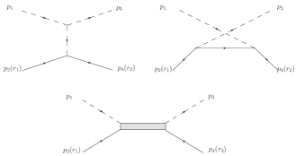
Figure 1: Model for the reaction $K^{-}p\to\eta\Lambda$. In these diagrams, we show the definition of the kinematical ($p_{1},p_{2},p_{3},p_{4}$) and polarization variables $r_{1},r_{2}$ that we use in our calculation.

The basic Feynman diagrams are shown in Fig. 1. These include $t-$channel $K^{*}$ exchange, $u-$channel proton exchange, and the $s-$channel $\Lambda(1670)(\equiv\Lambda^{*})$ terms. To compute the contributions of these terms, we use the interaction Lagrangian densities of Refs. wufq ; xie ; Mosel ; feuster :

$${\cal L}_{K^{*}K\eta} = g_{K^{*}K\eta}(\eta\partial^{\mu}{K^{-}}-K^{-}\partial^{\mu}{\eta})K^{*-}_{\mu}$$ (1)

$${\cal L}_{K^{*}N\Lambda} = g_{K^{*}N\Lambda}\bar{\Lambda}\big{(}\gamma_{\mu}-{\kappa\over 2M_{N}}\sigma_{\mu\nu}\partial^{\nu}\big{)}K^{*\mu}N$$ (2)

$$+\mathrm{H.c.}\,,$$

$${\cal L}_{\eta NN} = g_{\eta NN}{\bar{N}}\gamma_{5}N\eta,$$ (3)

$${\cal L}_{KN\Lambda} = g_{KN\Lambda}\bar{N}\gamma_{5}\Lambda K+\mathrm{H.c.},$$ (4)

$${\cal L}_{\Lambda^{*}{\bar{K}}N} = g_{\Lambda^{*}{\bar{K}}N}\bar{\Lambda}^{*}\bar{K}N+\mathrm{H.c.},$$ (5)

$${\cal L}_{\Lambda^{*}\Lambda\eta} = g_{\Lambda^{*}\Lambda\eta}\bar{\Lambda}^{*}\eta\Lambda+\mathrm{H.c.}.$$ (6)

where we take $\kappa=2.43$ that determined by the Nijmegen potential stoks99 and has been used in Ref. oh06 . Other coupling constants will be discussed below.

With the effective Lagrangian densities given above, we can easily construct the invariant scattering amplitudes:

$${\cal M}_{i}=\bar{u}_{r_{2}}(p_{4})~{}{\cal A}_{i}~{}u_{r_{1}}(p_{2}),$$ (7)

where $i$ denotes the $i$th channel that contributes to the total amplitude, and $\bar{u}_{r_{2}}(p_{4})$ and $u_{r_{1}}(p_{2})$ are the spinors of $\Lambda$ and proton, respectively. The reduced ${\cal A}_{i}$ read

$${\cal A}_{s} = g_{\Lambda^{*}{\bar{K}}N}g_{\Lambda^{*}\Lambda\eta}\frac{{\not\!p_{1}}+{\not\!p_{2}}+M_{\Lambda^{*}}}{s-M_{\Lambda^{*}}^{2}+iM_{\Lambda^{*}}\Gamma_{\Lambda^{*}}},$$ (8)

$${\cal A}_{t} = i\frac{g_{K^{*}K\eta}g_{K^{*}\Lambda N}}{q^{2}-m^{2}_{K^{*}}}({\not\!p_{1}}+{\not\!p_{3}}-\frac{m^{2}_{K}-m^{2}_{\eta}}{m^{2}_{K^{*}}}{\not\!q}$$ (9)

$$-\frac{\kappa}{m_{N}}(p_{1}\cdot p_{3}-{\not\!p_{1}}{\not\!p_{3}})),$$

$${\cal A}_{u} = -~{}g_{K\Lambda N}g_{\eta NN}\frac{{\not\!p_{2}}-{\not\!p_{3}}-m_{N}}{u-m^{2}_{N}}.$$ (10)

where $q$ is the momentum of exchanging meson $K^{*}$ in the $t-$channel. The width of $K^{*}$ is not taken into account since $K^{*}$ is in the $t-$channel. The subindices $s,t,$ and $u$ stand for the $s-$ channel $\Lambda^{*}$ exchange, $t-$channel $K^{*}$ exchange, and $u-$channel proton pole terms. As we can see, in the tree-level approximation, only the products like $g_{\Lambda^{*}{\bar{K}}N}g_{\Lambda^{*}\Lambda\eta}$, enter in the invariant amplitudes. They are determined with the use of MINUIT, by fitting to the experimental data data , including the total and differential cross sections. Besides, $M_{\Lambda^{*}}$ and $\Gamma_{\Lambda^{*}}$ are the mass and total decay width of the $\Lambda^{*}$ resonance, which are free parameters in the present work and will be also fitted to the experimental data.

Because we are not dealing with point-like particles, we ought to introduce the compositeness of the hadrons. This is usually achieved by including form factors in the amplitudes. In the present work, we adopt the following form factors wufq ; Mosel ; feuster

$$F(q_{ex}^{2},M_{ex})={\Lambda^{4}\over\Lambda^{4}+(q_{ex}^{2}-M_{ex}^{2})^{2}}\,,$$ (11)

for $s-$ and $u-$channel, and

$$F(q_{ex}^{2},M_{ex})=\left(\frac{\Lambda^{2}-M_{ex}^{2}}{\Lambda^{2}-q_{ex}^{2}}\right)^{2}\,,$$ (12)

for $t-$channel, where the $q_{ex}$ and $M_{ex}$ are the 4-momenta and the mass of the exchanged hadron, respectively. For the cutoff parameters, we take $\Lambda=2.0$ GeV for $s-$channel, $\Lambda=1.5$ GeV for $t-$ and $u-$channel.

The differential cross section for $K^{-}p\to\eta\Lambda$ at center of mass (c.m.) frame can be expressed as

$${d\sigma\over d{\rm cos}\theta_{\rm c.m.}}={1\over 32\pi s}{|\vec{p_{3}}^{\text{c.m.}}|\over|\vec{p_{1}}^{\text{c.m.}}|}\left({1\over 2}\sum_{r_{1},r_{2}}{|\cal M|}^{2}\right),$$ (13)

where $\theta_{\rm c.m.}$ denotes the angle of the outgoing $\eta$ relative to beam direction in the $\rm c.m.$ frame, and $s=(p_{1}+p_{2})^{2}$, is the invariant mass square of the system.

In Eq. (13), the total invariant scattering amplitude $\cal M$ is given by,

$${\cal M}={\cal M}_{s}+e^{i\theta_{1}}{\cal M}_{t}+e^{i\theta_{2}}{\cal M}_{u}\,.$$ (14)

In the phenomenological Lagrangian approaches, the relative phases between amplitudes from different diagrams are not fixed, so we introduce two relative phases $\theta_{1}$ and $\theta_{2}$ between the background and the $\Lambda^{*}$ contributions as free parameters, which will be determined by fitting to the experimental data.

We perform seven-parameter ($M_{\Lambda^{*}}$, $\Gamma_{\Lambda^{*}}$, $g_{\Lambda^{*}{\bar{K}}N}g_{\Lambda^{*}\Lambda\eta}$, $g_{K^{*}N\Lambda}g_{K^{*}K\eta}$, $g_{KN\Lambda}g_{\eta NN}$, $\theta_{1}$, and $\theta_{2}$) $\chi^{2}$ fit to the total and differential cross section data taken from Ref. data . There are a total $155$ data points.

The fitted parameters for $\Lambda(1670)$ are shown in Table. 1 and other fitted results are: $g_{K^{*}N\Lambda}g_{K^{*}K\eta}=14.8\pm 1.7$, $g_{KN\Lambda}g_{\eta NN}=-5.6\pm 0.9$, $\theta_{1}=2.9\pm 0.2$, and $\theta_{2}=2.9\pm 0.3$. The resultant $\chi^{2}/dof$ is $1.3$.

Table 1: Adjusted parameters for $\Lambda(1670)$ resonance. PDG estimates are also listed for comparison.

	Mass(MeV)	$\Gamma_{\mathrm{tot}}$(MeV)	$|g_{\Lambda^{*}{\bar{K}}N}g_{\Lambda^{*}\eta\Lambda}|$
This calculation	$1671.5\pm 0.2$	$23.3\pm 0.2$	$0.28\pm 0.03$
PDG	$1660\sim 1680$	$25\sim 50$	$0.31\pm 0.15$

On the other hand, the coupling constants of $g_{\Lambda^{*}{\bar{K}}N}$ and $g_{\Lambda^{*}\eta\Lambda}$ can be also evaluated from the $\Lambda(1670)$ to ${\bar{K}}N$ and $\eta\Lambda$ partial decay widths:

$$\Gamma_{\Lambda^{*}\to{\bar{K}}N} = \frac{g^{2}_{\Lambda^{*}{\bar{K}}N}}{2\pi}(E_{N}+m_{N})\frac{|\vec{p}_{N}|}{M_{\Lambda^{*}}},$$ (15)

$$\Gamma_{\Lambda^{*}\to\eta\Lambda} = \frac{g^{2}_{\Lambda^{*}\eta\Lambda}}{4\pi}(E_{\Lambda}+m_{\Lambda})\frac{|\vec{p}_{\Lambda}|}{M_{\Lambda^{*}}},$$ (16)

where

$$E_{N/\Lambda} = \frac{M^{2}_{\Lambda^{*}}+m^{2}_{N/\Lambda}-m_{{\bar{K}}/\eta}}{2M_{\Lambda^{*}}},$$ (17)

$$|\vec{p}_{N/\Lambda}| = \sqrt{E^{2}_{N/\Lambda}-m^{2}_{N/\Lambda}}\,.$$ (18)

With the value of total decay width $\Gamma_{\Lambda^{*}}=35\pm 15$ MeV, a value of $0.25\pm 0.05$ for the $\Lambda^{*}\to{\bar{K}}N$ branching ratio, and a value of $0.175\pm 0.075$ $\Lambda^{*}\to\eta\Lambda$ branching ratio, quoted in the Particle Data Group (PDG) book pdg2010 , we can get $|g_{\Lambda^{*}{\bar{K}}N}g_{\Lambda^{*}\eta\Lambda}|=0.31\pm 0.15$, which was also shown in Table. I for comparison. The error $\pm 0.15$ is came from that the errors of the $\Lambda^{*}\to{\bar{K}}N$ and $\Lambda^{*}\to\eta\Lambda$ partial decay widths.

As we can see in Table. I, the fitted parameters for the $\Lambda(1670)$ resonance agree well with that of the PDG estimation.

During the best fit, we adjusted the product of the coupling constants to experimental data. If we take $g_{K^{*}K\eta}=1.6$ that was obtained from the $SU(3)$ prediction wufq , then we can get $|g_{K^{*}N\Lambda}|=9.3\pm 1.0$ which roughly agrees with the value, $|g_{K^{*}N\Lambda}|=6.1$, which was obtained from the $SU(3)$ flavor symmetry in Ref. stoks99 . Since the value of $g_{\eta NN}$ is extremely uncertain and if we adopt it as $2.24$ that was used in Ref. xie , then we get $|g_{KN\Lambda}|=2.5\pm 0.5$ which is much different with the $SU(3)$ prediction value $13.3$ ohprt06 ; oh08 . However, as we mentioned above, the uncertainty of $g_{\eta NN}$ is very large nneta1 ; nneta2 ; nneta3 ; nneta4 ; nneta5 ; nneta6 , so the adjusted coupling constant $g_{KN\Lambda}$, in the present work, may be still within the $SU(3)$ prediction.

Our best fits to the experimental data of the total cross sections are shown in Fig. 2, comparing with the data. The solid line represents the full results, while the contribution from $\Lambda(1670)$, $t-$, and $u-$channel diagrams are shown by the dotted, dashed and dot-dot-dashed lines, respectively. From Fig. 2, one can see that we can describe the data of total cross sections quite well and the $\Lambda(1670)$ gives the dominant contribution, while the $t-$ and $u-$channel diagrams give the minor but sizeable contribution.

Figure 2: $K^{-}p\to\eta\Lambda$ total cross sections compared with the data data . Results have been obtained from the best $\chi^{2}$ fit. The solid line represents the full results, while the contribution from $\Lambda(1670)$, $t-$, and $u-$channel diagrams are shown by the dotted, dashed and dot-dot-dashed lines, respectively. The dot-dashed represents the best results for the total cross sections after including the $D_{03}$ state.

The results of the best fit for the differential cross sections are shown with the solid line in Fig. 3. From there we can see that the deviations between our theoretical results and experimental data are evident especially for the angular distribution at $p_{K^{-}}=730,732,734,738,742$ MeV, where bowl-shaped structures in angular dependence appear. It also should be noted that with including the background contribution from the $t-$channel $K^{*}$ exchange and $u-$channel proton exchange, the backward enhancement in the angular distribution for $p_{K^{-}}$ from $750$ to $770$ MeV are reproduced.

Figure 3: The best fitting results for differential cross sections. The solid lines represent the results by considering only $\Lambda(1670)$ and background contributions, while the dashed lines represents the result by including also a narrow $D_{03}$ resonance.

In order to obtain a better description of the differential cross section data, especially at some energy points, some other resonances that may contribute to this reaction should also be considered. For the bowl structures in differential cross sections, one possible explanation is that there might be $d-$wave contributions from the $s-$channel with the excitation of $D_{03}$ resonance. For checking this, we performed another best fit: in addition to the contributions which were already considered in the previous fit, the contribution from the $D_{03}$ state in the $s-$channel process are also included. The new best fitting gives $\chi^{2}/dof=0.9$ and we get a satisfied description for both total cross sections and differential cross sections. The new results for the total cross sections are similar with the previous results except for a small bump around $p_{K^{-}}=736$MeV(see the dot-dashed line in Fig. 2). The corresponding results for differential cross sections are shown with dotted line in Fig. 3, where the bowl structures are well reproduced.

The fitted parameters for $D_{03}$ resonance are mass $M=1668.5\pm 0.5$ MeV and total decay width $\Gamma=1.5\pm 0.5$ MeV. The mass of $D_{03}$ is close to the PDG estimate for $\Lambda(1690)$ ($M_{\Lambda(1690)}=1690\pm 5$ MeV), while the width is too small compared to the PDG estimate ($\Gamma_{\Lambda(1690)}=60\pm 10$ MeV). The width obtained from the best fit is narrow because the bowl structures in the differential cross sections are shown up in a narrow ($\pm 3$ MeV)  energy window.

One might think that releasing the limit of the cutoff values for the form factors and inclusion of more $\Lambda$ resonances (such as $\Lambda(1600)$) might improve the situation that the width of the $D_{03}$ state is too narrow. We have explored such possibility, but we have found tiny changes. The new best fitting still favor a $D_{03}$ resonance with very small width and the corresponding values for the parameters of $D_{03}$ resonance are close to the values that were obtained above.

In summary, we have studied the $K^{-}p\to\eta\Lambda$ reaction near threshold by using an effective Lagrangian approach. The role of the $s-$channel $\Lambda(1670)$, $t-$channel $K^{*}$ and $u-$channel proton pole diagrams are considered. The total cross section are well reproduced. Our results show that $\Lambda(1670)$ gives the dominant contribution, while the $t-$ and $u-$channel diagrams give the minor but sizeable contribution, especially for the backward enhancement in the angular distribution for $p_{K^{-}}$ from $750$ to $770$ MeV.

However, including $\Lambda(1670)$ resonance in the $s-$channel as well as the background contributions is not enough to describe the bowl structures in the angle distributions at some beam momentum points. A general opinion is that these bowl structures in angular distribution can be understood by further including the contribution from $\Lambda(1690)D_{03}$. Indeed, our calculations show that with considering the $D_{03}$ resonance, we can describe the bowl structures, but a rather small width of this resonance is needed. This means that the experimental data can not be understood by considering the conventional $\Lambda(1690)$. On the other hand, the current experimental data still have systematic uncertainties especially when we look at the angular distribution data obtained from two different ways of identifying the final $\eta$ meson(see Fig. 20 of Ref. data ), so the present results give a signal for the needs of further studies in this reaction.

References

- (1) A. Starostin, et al., Phys. Rev. C64, 055205 (2001).
- (2) K. Nakamura et al., J. Phys. G37, 075021 (2010).
- (3) P. Z. Gao, B. S. Zou and A. Sibirtsev, Nucl. Phys. A867, 41 (2011) .
- (4) E. Oset, A. Ramos, C. Bennhold, Phys. Lett. B527, 99 (2002).
- (5) C. Garcia-Recio, J. Nieves, E. Ruiz Arriola and M. J. Vicente Vacas, Phys. Rev. D66, 076009 (2003).
- (6) Xian-Hui Zhong, and Qiang Zhao, Phys. Rev. C79, 045202 (2009).
- (7) F. Q. Wu, B. S. Zou, L. Li and D. V. Bugg, Nucl. Phys. A735, 111 (2004); F. Q. Wu, and B. S. Zou, Phys. Rev. D73, 114008 (2006).
- (8) J. J. Xie, B. S. Zou and H. Q. Jiang, Phys. Rev. C77, 015206 (2008).
- (9) G. Penner and U. Mosel, Phys. Rev. C66, 055211 (2002); ibid. C66, 055212 (2002); V. Shklyar, H. Lenske and U. Mosel, Phys. Rev. C72, 015210 (2005).
- (10) T. Feuster and U. Mosel, Phys. Rev. C58, 457 (1998); Phys. Rev. C59, 460 (1999).
- (11) V. G. J. Stoks and Th. A. Rijken, Phys. Rev. C59, 3009 (1999).
- (12) Y. Oh and H. Kim, Phys. Rev. C73, 065202 (2006).
- (13) Y. Oh, K. Nakayama, and T. S. H. Lee, Phys. Rep 423, 49 (2006).
- (14) Y. Oh, C. M. Ko, and K. Nakayama, Phys. Rev. C77, 045204 (2008).
- (15) W. Grein and P. Kroll, Nucl. Phys. A338, 332 (1980).
- (16) M. Kirchbach and L. Tiator, Nucl. Phys. A604, 385 (1996).
- (17) S. L. Zhu, Phys. Rev. C61, 065205 (2000).
- (18) G. Faldt and C. Wilkin, Phys. Scr. 64, 427 (2001).
- (19) L. Tiator, C. Bennhold, and S. S. Kamalov, Nucl. Phys. A580, 455 (1994).
- (20) K. Nakayama, Y. Oh, and H. Haberzettl, J. Korean Phys. Soc.59, 224 (2011).