Decorated Shastry-Sutherland lattice in the spin-$\frac{1}{2}$ magnet CdCu₂(BO₃)₂

Abstract

We report the microscopic magnetic model for the spin-$\frac{1}{2}$ Heisenberg system CdCu₂(BO₃)₂, one of the few quantum magnets showing the $\frac{1}{2}$-magnetization plateau. Recent neutron diffraction experiments on this compound $[$M. Hase et al., Phys. Rev. B 80, 104405 (2009)$]$ evidenced long-range magnetic order, inconsistent with the previously suggested phenomenological magnetic model of isolated dimers and spin chains. Based on extensive density-functional theory band structure calculations, exact diagonalizations, quantum Monte Carlo simulations, third-order perturbation theory, as well as high-field magnetization measurements, we find that the magnetic properties of CdCu₂(BO₃)₂ are accounted for by a frustrated quasi-2D magnetic model featuring four inequivalent exchange couplings: the leading antiferromagnetic coupling $J_{\text{d}}$ within the structural Cu₂O₆ dimers, two interdimer couplings $J_{\text{t1}}$ and $J_{\text{t2}}$, forming magnetic tetramers, and a ferromagnetic coupling $J_{\text{it}}$ between the tetramers. Based on comparison to the experimental data, we evaluate the ratios of the leading couplings $J_{\text{d}}$ : $J_{\text{t1}}$ : $J_{\text{t2}}$ : $J_{\text{it}}$ = 1 : 0.20 : 0.45 : $-$0.30, with $J_{\text{d}}$ of about 178 K. The inequivalence of $J_{\text{t1}}$ and $J_{\text{t2}}$ largely lifts the frustration and triggers long-range antiferromagnetic ordering. The proposed model accounts correctly for the different magnetic moments localized on structurally inequivalent Cu atoms in the ground-state magnetic configuration. We extensively analyze the magnetic properties of this model, including a detailed description of the magnetically ordered ground state and its evolution in magnetic field with particular emphasis on the $\frac{1}{2}$-magnetization plateau. Our results establish remarkable analogies to the Shastry-Sutherland model of SrCu₂(BO₃)₂, and characterize the closely related CdCu₂(BO₃)₂ as a material realization for the spin-$\frac{1}{2}$ decorated anisotropic Shastry-Sutherland lattice.

I Introduction

Among the great variety of magnetic ground states (GSs), only few can be rigorously characterized using analytical considerations. To these exceptional cases belong, e.g., the Heisenberg zigzag chain model at the so-called Majumdar–Ghosh point,Majumdar and Ghosh (1969a); *FHC_AFAF_GS_2 a class of Kitaev models,Kitaev (2006) as well as the dimerized phase of the Heisenberg model on the Shastry-Sutherland lattice.Shastry and Sutherland (1981) The latter describes the magnetism of $S$ = 1/2 spins on a square lattice, with two inequivalent exchange couplings: (i) a dimer-like coupling $J$ connecting the spins pairwise along the diagonals of the square lattice, and (ii) the coupling $J^{\prime}$ along the edges of the square lattice (Fig. 1, left). For the ratio of antiferromagnetic (AFM) couplings $J^{\prime}$/$J$ $<$ 0.7, the GS is an exact product of singlets residing on the $J$ bonds.Miyahara and Ueda (1999)

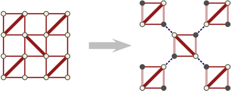
Figure 1: (Color online) Left panel: the original Shastry-Sutherland model with the dimer-like coupling $J$ (thick lines) and the coupling $J^{\prime}$ (thin lines) along the edges of the square lattice. Right panel: the decorated anisotropic Shastry-Sutherland model in CdCu₂(BO₃)₂. The horizontal and vertical couplings ($J^{\prime}$ in the original model) are not equivalent, leading to $J_{\text{t1}}$ (double line) and $J_{\text{t2}}$ (single line). In addition, the coupling $J_{\text{t1}}$ (dashed line) tiles the lattice into four-spin units (tetramers). Filled circles denote the decorating spins.

The Shastry-Sutherland model was first studied theoretically,Shastry and Sutherland (1981) and only two decades later the spin $S$ = $\frac{1}{2}$ magnet SrCu₂(BO₃)₂ was claimed to be an experimental realization of this model.Kageyama et al. (1999) In the following years, numerous experimental and theoretical studies disclosed a rather complex magnetic behavior of this compound, including plateaux at 1/8, 1/4, and 1/3 of the saturation magnetization (Ref. Onizuka et al., 2000) and an intricate coupling between magnetic and lattice degrees of freedom.Vecchini et al. (2009) For the experimentally defined ratio of the leading couplings $J^{\prime}$/$J$ = 0.64 (Refs. Miyahara and Ueda, 2000 and Miyahara and Ueda, 2003), the system is already in the dimerized singlet phase, but very close to the quantum critical point.[See; e.g.; Ref.~\cite[citep]{\@@bibref{AuthorsPhrase1Year}{SCBO_theory_review}{\@@citephrase{; }}{}}; ][]SCBO_GS_SE; *SCBO_CCM To access the critical point, further tuning of the system is required. For example, external pressure leads to at least one phase transition at low temperatures,Waki et al. (2007) as evidenced by nuclear magnetic resonance (NMR) studies,[Forarecentreview; see][]SCBO_NMR_review while a recent theoretical modelMoliner et al. (2011) with two inequivalent dimer couplings $J$ predicts an unanticipated, effectively one-dimensional Haldane phase.Moliner et al. (2011); Ivanov and Richter (1997)

An alternative way to tune the magnetic couplings is the directed substitution of nonmagnetic atoms or anionic groups. The impact of this substitution on the magnetic coupling regime can be very different. The simplest effect is a bare change of the energy scale, which does not affect the physics, as for instance, in the spin-$\frac{1}{2}$ uniform-chain compounds Sr₂Cu(PO₄)₂ and Ba₂Cu(PO₄)₂.Belik et al. (2004); *HC_Sr2CuPO42_DFT_chiT_fit Another possibility is alteration of the leading couplings, as in the frustrated square lattice systems $AA^{\prime}$VO(PO₄)₂ (Ref. Tsirlin and Rosner, 2009) or the kagome lattice compounds kapellasite Cu₃Zn(OH)₆Cl₂ and haydeeite Cu₃Mg(OH)₆Cl₂.Colman et al. (2008); *kapel_hayd_DFT; *kapel_hayd_str_neutr Such systems have excellent potential for exploring magnetic phase diagrams. Finally, in some cases, chemical substitutions drastically alter the underlying magnetic model, as shown recently for the family of Cu${}_{2}A_{2}$O₇ compounds ($A$ = P, As, V).Janson et al. (2011); *Cu2V2O7_DFT; *Cu2As2O7

However, the most common effect of chemical substitution is a structural transformation, which apparently leads to a major qualitative change in the magnetic couplings. For instance, the Se–Te substitution, accompanied by a major structural reorganization, transforms the Heisenberg-chain system CuSe₂O₅ (Ref. Janson et al., 2009) into the spin dimer compound CuTe₂O₅ (Ref. Deisenhofer et al., 2006; *CuTe2O5_DFT_fchiT_fCpT_fMH). Likewise, the La–Bi substitution in the 2D square lattice system La₂CuO₄ (Ref. Pickett, 1989) leads to the three-dimensional magnet Bi₂CuO₄ (Ref. Janson et al., 2007), etc.

Coming back to the $S$ = $\frac{1}{2}$ Shastry-Sutherland compound SrCu₂(BO₃)₂, the directed substitution of nonmagnetic structural elements is an appealing tool to explore the phase space of the Shastry-Sutherland model.Choi et al. (2003); *SCBO_met_doping_chiT; *SCBO_Zn_Si_doping_chiT_MH; *SCBO_Mg_doping_INS One possible way is the replacement of Sr²⁺ by another divalent cation. Indeed, the compound CdCu₂(BO₃)₂ exists, and its magnetic properties have been investigated experimentally.Hase et al. (2005); Mitsudo et al. (2007); Hase et al. (2009) In contrast to SrCu₂(BO₃)₂, the magnetic GS of CdCu₂(BO₃)₂ is long-range ordered, while the magnetization $M(H)$ curve exhibits a plateau at one-half of the saturation magnetization.Hase et al. (2005)

The substitution of Sr by Cd in SrCu₂(BO₃)₂ is accompanied by a structural transformation. Thus, the initial tetragonal symmetry is reduced to monoclinic, engendering two independent magnetic sites: Cu(1) and Cu(2). The presence of Cu(1) residing in the structural dimers, similar to SrCu₂(BO₃)₂, and the relatively short Cu(2)–Cu(2) connections along $c$ motivated the authors of Ref. Hase et al., 2005 to advance a tentative magnetic model comprising isolated magnetic dimers of Cu(1) pairs and infinite chains built by Cu(2) spins. This model was in agreement with the experimental magnetic susceptibility $\chi(T)$, magnetization $M(H)$, and electron spin resonance (ESR) data. However, later neutron diffraction (ND) studies challenged this model, since the ordered magnetic moments localized on Cu(1) amount to 0.45 $\mu_{\text{B}}$ compared to 0.83 $\mu_{\text{B}}$ on Cu(2).Hase et al. (2009) Therefore, the Cu(1) dimers do not form a singlet state with zero ordered moment, but rather experience a sizable coupling to Cu(2). This coupling is ferromagnetic, as inferred from the magnetic structure, and contrasts with the AFM coupling assumed in the previous studies.Hase et al. (2005)

The tentative magnetic model from Ref. Hase et al., 2005 was founded on the assumption that the strongest magnetic couplings are associated with the shortest Cu–Cu interatomic distances. However, such an approach fully neglects the mutual orientation of magnetic orbitals, which play a decisive role for the magnetic coupling regime. Moreover, the experimental results suggest that the actual spin model of CdCu₂(BO₃)₂ is more complex than the simple “chain + dimer” scenario.

In this paper, we investigate the magnetic properties of CdCu₂(BO₃)₂ on a microscopic level, using density-functional-theory (DFT) band structure calculations, exact diagonalization (ED) and quantum Monte Carlo (QMC) numerical simulations, as well as analytical low-energy perturbative expansions and linear spin-wave theory. We show that the magnetism of CdCu₂(BO₃)₂ can be consistently described by a two-dimensional (2D) frustrated isotropic model (crystalline and exchange anisotropy effects are neglected) with four inequivalent exchange couplings, topologically equivalent to the decorated anisotropic Shastry-Sutherland lattice (see Fig. 1, right). Therefore, the chemical similarity between SrCu₂(BO₃)₂ and CdCu₂(BO₃)₂  is retained on the microscopic level. The dominance of the exchange interaction $J_{\text{d}}$ within the structural Cu(1) dimers allows to describe the magnetic properties within an effective low-energy model for the Cu(2) sites only. This effective model explains the sizable staggered magnetization of Cu(1) dimers despite the large $J_{\text{d}}$, and unravels the nature of the wide 1/2-magnetization plateau in CdCu₂(BO₃)₂. The experimental data, both original and taken from the literature, are reconsidered in terms of the DFT-based microscopic model and the effective model. As a result, we find an excellent agreement between the simulated and measured quantities.

This paper is organized as follows. Sec. II is devoted to the discussion of the structural peculiarities of CdCu₂(BO₃)₂. The methods used in this study are presented in Sec. III. Then, the microscopic magnetic model is evaluated using DFT band structure calculations, and its parameters are refined using ED fits to the experiments (Sec. IV). The magnetic properties of CdCu₂(BO₃)₂ are in the focus of Sec. V. We show that the magnetism of CdCu₂(BO₃)₂ is captured by an effective low-energy description of the Cu(2) spins (on the Shastry-Sutherland lattice), which are further studied using linear spin-wave theory as well as QMC, and corroborated by ED for the microscopic magnetic model. Finally, in Sec. VI a summary and a short outlook are given.

II Crystal structure

The low-temperature crystal structure of CdCu₂(BO₃)₂ is reliably established based on synchrotron x-ray and neutron diffraction data.Hase et al. (2009) The basic structural elements of CdCu₂(BO₃)₂ are magnetic layers (Fig. 2) that stretch almost parallel to $(\bar{1}02)$ planes (Fig. 2, right bottom). These layers are formed by Cu–O polyhedra coupled by B₂O₅ units.

Although Cd²⁺ is isovalent to Sr²⁺, the substantial difference in their ionic radii (1.26 Å and 0.95 Å, respectively)Shannon (1976) gives rise to different structural motives in the two systems. Thus, in sharp contrast with SrCu₂(BO₃)₂, the monoclinic crystal structure of CdCu₂(BO₃)₂ comprises two inequivalent positions for Cu atoms: Cu(1) and Cu(2). The local environment of these two sites is different: Cu(1) forms Cu(1)O₄ plaquettes that in turn build structural Cu(1)₂O₆ dimers, resembling SrCu₂(BO₃)₂, while Cu(2) atoms form tetrahedrally distorted Cu(2)O₄ plaquettes that share a common O atom with the Cu(1)₂O₆ dimers (Fig. 2). As a result, structural Cu(1)₂Cu(2)₂O₁₂ tetramers are formed. Interestingly, the structural tetramers do not coincide with the magnetic tetramers (shaded oval in Fig. 2) that are the basic units of the spin lattice (Sec. IV.1).

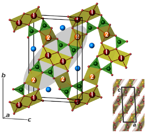
Figure 2: (Color online) The crystal structure of CdCu₂(BO₃)₂ consists of structural Cu(1)₂O₆ dimers, Cu(2)O₄ distorted plaquettes, BO₃ triangles connected pairwise as well as isolated Cd atoms (spheres). Oxygen atoms are shown as small spheres located at the vertices of Cu(1)O₄, Cu(2)O₄ and BO₃ polyhedra. The numbers “1” and “2” denote Cu(1) and Cu(2), respectively. A magnetic tetramer (see Sec. IV.1) is shaped by a gray oval. Right bottom: position of the magnetic layers (shaded) in the crystal structure of CdCu₂(BO₃)₂.

Large cavities between the neighboring magnetic tetramers accommodate Cd atoms. As a result, the space between the magnetic layers is rather narrow, leading to short interatomic distances ($\sim$3.4 Å) between the Cu atoms belonging to neighboring magnetic layers. On the basis of such short Cu–Cu distance, the relevance of the respective interlayer coupling (the chain-like coupling $J_{3}$ in the notation of Ref. Hase et al., 2005) has been conjectured.Hase et al. (2005) However, the orientation of magnetic Cu(1)₂O₆ and Cu(2)O₄ polyhedra (almost coplanar to the magnetic layers) excludes an appreciable interlayer coupling. This quasi-2D scenario is readily confirmed by our DFT calculations (Sec. IV.1).

The evaluation of the intralayer coupling based on structural considerations is more involved. In many cuprates, the leading exchange couplings are typically associated with the Cu–O${}_{\text{plaq}}$–Cu connections, i.e., when the neighbouring plaquettes share a common corner (one O${}_{\text{plaq}}$ atom) or a common edge (two O${}_{\text{plaq}}$ atoms). In the crystal structure of CdCu₂(BO₃)₂, both types of connections are present.

To estimate the respective magnetic exchange couplings, the Goodenough–Kanamori rulesGoodenough (1955); *GKA_2 are typically applied. Using a closely related approach, Braden et al.Braden et al. (1996) evaluated the dependence of the magnetic exchange $J$ on the Cu–O–Cu angle. According to their results, for the Cu–O–Cu angle of 90^∘, the resulting total coupling $J$, being a sum of AFM $J^{\text{AFM}}$ (positive) and FM $J^{\text{FM}}$ (negative) contributions, is FM. An increase in this angle (i) decreases the $J^{\text{FM}}$ contribution caused by Hund’s coupling on the O sites,Mazurenko et al. (2007) and (ii) enhances the Cu–O–Cu superexchange which in turn increases $J^{\text{AFM}}$. As a result, for the Cu–O–Cu angle close to 97^∘, $J^{\text{FM}}$ and $J^{\text{AFM}}$ are balanced, thereby cancelling the total magnetic exchange ($J$ = 0). Further increase in the Cu–O–Cu angle breaks this subtle balance and gives rise to an overall AFM exchange, which grows monotonically up to Cu–O–Cu = 180^∘.

Here, we try to apply this phenomenological approach and estimate the respective exchange integrals. The intradimer Cu(1)–O–Cu(1) angle in CdCu₂(BO₃)₂ is 98.2^∘, only slightly exceeding 97^∘. Therefore, a weak AFM exchange coupling could be expected. For the Cu(1)–O–Cu(2) corner-sharing connections, the angle amounts to 117.5^∘, which should give rise to a sizable AFM exchange. However, our DFT+$U$ calculations deliver a magnetic model, which is in sharp contrast with these expectations: the AFM coupling within the structural dimers is sizable, while the coupling along the Cu(1)–O–Cu(2) connections is much smaller and FM. The substantial discrepancy between the simplified picture, based on structural considerations only, and the microscopic model, evidences the crucial importance of a microscopic insight for structurally intricate magnets like CdCu₂(BO₃)₂.

III Methods

DFT band structure calculations were performed using the full-potential code fplo-8.50-32.Koepernik and Eschrig (1999) For the structural input, we used the atomic positions based on the neutron diffraction data at 1.5 K: space group $P2_{1}/c$ (14), $a$ = 3.4047 Å, $b$ = 15.1376 Å, $c$ = 9.2958 Å, $\beta$ = 92.807^∘.Hase et al. (2009) For the scalar-relativistic calculations, the local-density approximation (LDA) parameterization of Perdew and Wang has been chosen.Perdew and Wang (1992) We also cross-checked our results by using the parameterization of Perdew, Burke and Ernzerhof based on the generalized gradient approximation (GGA).Perdew et al. (1996) For the nonmagnetic calculations, a $k$mesh of 30$\times$6$\times$12 = 2160 points (728 points in the irreducible wedge) has been adopted. Wannier functions (WF) for the Cu $3d_{x^{2}-y^{2}}$ states were evaluated using the procedure described in Ref. Eschrig and Koepernik, 2009. For the supercell magnetic DFT+$U$ calculations, two types of supercells were used: a supercell metrically equivalent to the unit cell (sp. gr. $P1$, 4$\times$2$\times$2 $k$mesh) and a supercell doubled along $c$ (sp. gr. $P1$, 4$\times$1$\times$1 $k$mesh). Depending on the double-counting correction (DCC),Czyżyk and Sawatzky (1994); *LSDA+U_Pickett the around-mean-field (AMF) or the fully localized limit (FLL), we varied the on-site Coulomb repulsion parameter $U_{3d}$ in a wide range: $U_{3d}$ = 5.5–7.5 eV for the AMF and $U_{3d}$ = 8.5–10.5 eV for the FLL calculations, keeping $J_{3d}$ = 1 eV. The local spin-density approximation (LSDA)+$U$ results were cross-checked by GGA+$U$ calculations. All results were accurately checked for convergence with respect to the $k$mesh.

Full diagonalizations of the resulting Heisenberg Hamiltonian were performed using the software package alps-1.3 (Ref. Albuquerque et al., 2007) on the $N$ = 16 finite lattice with periodic boundary conditions. Translational symmetries have been used (the code does not allow for rotational symmetries). Spin correlations in the GS as well as the lowest-lying excitations were computed by Lanczos diagonalization of $N$ = 32 sites finite lattices using the code spinpack.Schulenburg Translational symmetries and the commutation relation $[H,S_{z}]$ = 0 were used. The finite lattices are depicted in Fig. 12. The QMC simulations of the effective model were performed on finite lattices with up to $N$ = 2304 spins with periodic boundary conditions using the looperTodo and Kato (2001) algorithm from the ALPS package.Albuquerque et al. (2007) For $T$ = 0.05 $J$ $\simeq$ 0.0031 $J_{\text{d}}$($\simeq$ 0.55 K), we used 40 000 loops for thermalization and 400 000 loops after thermalization.

A powder sample of CdCu₂(BO₃)₂ was prepared by annealing a stoichiometric mixture of CuO, CdO, and B₂O₃ in air at 750 ^∘C for 96 hours. The sample contained trace amounts of unreacted CuO and Cd₂B₂O₅ (below 1 wt.% according to the Rietveld refinement), as evidenced by powder x-ray diffraction (Huber G670 camera, CuK_α1 radiation, ImagePlate detector, $2\theta$ = 3–100^∘ angle range). To improve the sample quality, we performed additional annealings that, however, resulted in a partial decomposition of the target CdCu₂(BO₃)₂ phase. Both impurity phases reveal a low and nearly temperature-independent magnetization within the temperature range under investigation. Therefore, they do not affect any of the results presented below.

The magnetic susceptibility ($\chi$) was measured with an MPMS SQUID magnetometer in the temperature range $2-380$ K in applied fields up to 5 T. The high-field magnetization curve was measured in pulsed magnetic fields up to 60 T at a constant temperature of 1.5 K using the magnetometer installed at the Dresden High Magnetic Field Laboratory. Details of the experimental procedure can be found in Ref. Tsirlin et al., 2009.

IV Evaluation of a microscopic magnetic model

IV.1 Band structure calculations

We begin our analysis with the evaluation of the magnetically relevant orbitals and couplings. The LDA yields a valence band with a width of about 9 eV, dominated by O $2p$ states (Fig. 3, top panel). Interestingly, the lower part of the valence band exhibits sizable contribution from the Cd $4d$ states, hinting at an appreciable covalency of Cd–O bonds. The energy range between $-3$ and $0.5$ eV is dominated by Cu $3d$ states. The presence of bands crossing the Fermi level evidences a metallic GS, which contrasts with the emerald-green color of CdCu₂(BO₃)₂. This well-known shortcoming of the LDA and the GGA originates from underestimation of strong correlations, intrinsic for the $3d^{9}$ electronic configuration of Cu²⁺. To remedy this drawback, we use two approaches accounting for the missing part of correlations: (i) on the model level, via mapping the LDA bands onto a Hubbard model (model approach); and (ii) directly within a DFT code, by adding an energy penalty $U_{3d}$ for two electrons occupying the same orbital (DFT+$U$ approach).

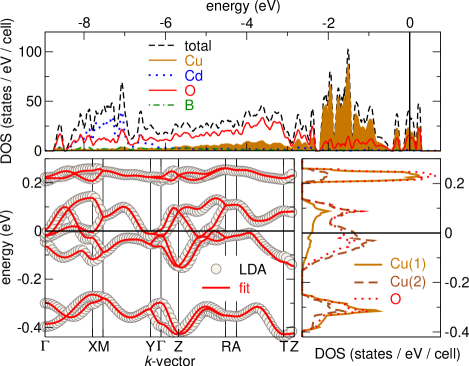
Figure 3: (Color online) Top: LDA valence band of CdCu₂(BO₃)₂. Atom-resolved DOS (number of states per eV and crystallographic unit cell) are shown. Bottom left: LDA band structure of the well-separated eight-band complex at the Fermi level and the WF tight-binding fit within an effective one-orbital model. Bottom right: atom-resolved DOS of the eight-band complex.

The states relevant for magnetism are located in a close vicinity of the Fermi level. Common for cuprates, these states form a band complex, well-separated from the rest of the valence band. This band complex, depicted in Fig. 3 (bottom panels), comprises eight bands, in accord with the eight Cu atoms in a unit cell. The projection of these states onto a local coordinate system readily yields their orbital character: typical for cuprates, these states correspond to the antibonding $\sigma$-combination of Cu $3d_{x^{2}-y^{2}}$ and O $2p$ orbitals. To visualize this combination in real space, the WFs for Cu $3d_{x^{2}-y^{2}}$ states can be used (Fig. 4).

To evaluate the relevant couplings, we calculate hopping matrix elements of the WFs and introduce them as parameters ($t_{i}$) into an effective one-orbital tight-binding model. This parameterization is justified by an excellent fit (Fig. 3, bottom left) to the LDA band dispersions. The relevant couplings ($t_{i}$ $>$ 20 meV) are presented in Table 1 (third column).

The transfer integrals $t_{i}$ can be subdivided into four groups, according to their strength. The first group contains only one term $t_{\text{d}}$ (“d” stands for “dimer”), which clearly dominates over all other couplings, despite the respective Cu(1)–O–Cu(1) angle being rather close to 90^∘. The second group comprises two terms, $t_{\text{t1}}$ and $t_{\text{t2}}$ (“t” stands for “tetramer”) that couple Cu(1) and Cu(2) atoms via Cu(1)–O–O–Cu(2) paths (Fig. 4) within the magnetic tetramers. Although the Cu(1)–Cu(2) distance for $t_{\text{t1}}$ is shorter, the respective coupling is slightly smaller than $t_{\text{t2}}$. This difference plays an important role for the magnetism of CdCu₂(BO₃)₂, as will be shown later.

The couplings $t_{\text{d}}$, $t_{\text{t1}}$, and $t_{\text{t2}}$ form magnetic tetramers (shaded oval in Fig. 2). These tetramers are coupled to each other by two interactions forming the third group: $t_{\text{it}}$ and $t_{\text{Cd}}$. The coupling $t_{\text{it}}$ (‘it” stands for “intertetramer”) corresponds to the magnetic exchange $J_{2}$ between dimers and chains in the notation of Ref. Hase et al., 2005. It is short-ranged, and runs via the corner-sharing Cu(1)–O–Cu(2) connection. The second intertetramer term $t_{\text{Cd}}$ couples Cu(1) and Cu(2) via Cd atoms (not shown). Finally, the fourth group of transfer integrals includes all other terms that are smaller than 20 meV. Since these latter terms play a minor role for the magnetic properties of CdCu₂(BO₃)₂, they are disregarded in the following discussion.

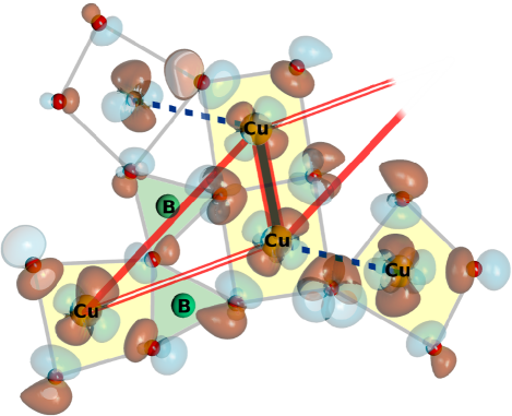
Figure 4: (Color online) Wannier functions for the Cu $3d_{x^{2}-y^{2}}$ states. Light and dark areas (colors) denote different phases of the functions. Relevant exchange couplings are depicted by lines: thick (red-black) lines ($J_{\text{d}}$), thinner solid ($J_{\text{t2}}$) and double ($J_{\text{t1}}$) lines, as well as dashed lines ($J_{\text{it}}$). Note the Cu–O–O–Cu superexchange paths via the BO₃ triangles.

Table 1: Cu–Cu distances ($d$, in Å), transfer integrals ($t_{i}$, in meV), antiferromagnetic $J_{i}^{\text{AFM}}$ (in K) contributions, as well as the total exchange integrals $J_{i}$ (in K) for the leading couplings in CdCu₂(BO₃)₂. The values of $J_{i}$ are evaluated within the DFT+$U$ method for two different double-counting correction schemes with $U_{3d}$ = 6.5 eV for AMF and 9.5 eV for FLL.

exchange	$d$	$t_{i}$		$J_{i}^{\text{AFM}}$		$J_{i}$ (LSDA+$U$)
						AMF		FLL
$J_{\text{d}}$	2.957	203		425		146		202
$J_{\text{t1}}$	5.268	73		55		30		29
$J_{\text{t2}}$	6.436	85		75		64		55
$J_{\text{it}}$	3.228	47		23		$-$45		$-$135
$J_{\text{Cd}}$	6.450	41		17		5		6
$J_{\text{t1}}$ : $J_{\text{d}}$ (%)						20		14
$J_{\text{it}}$ : $J_{\text{d}}$ (%)						$-31$		$-67$
$J_{\text{t1}}$ : $J_{\text{t2}}$ (%)						47		53

To account for electronic correlations, neglected in the tight-biding model, the transfer integrals $t_{i}$ are mapped onto a Hubbard model. This way, under the conditions of half-filling and strong correlations ($U_{\text{eff}}$ $\gg$ $t_{i}$), the AFM contribution $J_{i}^{\text{AFM}}$ to the exchange integrals can be estimated in second-order perturbation theory:Anderson (1959) $J_{i}^{\text{AFM}}$ = $4t_{i}^{2}/U_{\text{eff}}$. Here, $U_{\text{eff}}$ is an effective term which takes into account the correlations in the magnetic Cu $3d_{x^{2}-y^{2}}$ orbitals, screened by the O $2p$ orbitals (their strong hybridization can be seen in Fig. 4). Although the experimental evaluation of $U_{\text{eff}}$ is challenging (see, e.g., Ref. Neudert et al., 2000), there is an empirical evidence that $U_{\text{eff}}$ values in the 4–5 eV range yield reasonable results for Cu²⁺ compounds.Johannes et al. (2006); Janson et al. (2009, 2007) Here, we adopt $U_{\text{eff}}$ = 4.5 eV to estimate $J_{i}^{\text{AFM}}$ (Table 1, fourth column).

Resorting from $t_{i}$ to $J_{i}^{\text{AFM}}$ basically preserves the picture of coupled tetramers with a strong dimer-like coupling. However, the interatomic Cu-Cu distances for $J_{\text{d}}$ and $J_{\text{it}}$ are rather small, thus sizable FM contributions to these couplings can be expected. To account for the FM exchange, we perform DFT+$U$ calculations for different magnetic supercells,[StrongcorrelationsinherenttotheCu$3d^9$electronicconfigurationensuretheapplicabilityoftheDFT+$U$methods; see; e.g.][]LDA+U_GW_compar and subsequently map the resulting total energies onto a Heisenberg model. This way, the FM contribution can be evaluated by subtracting $J_{i}^{\text{AFM}}$ estimates from the values of the total exchange $J_{i}$, obtained from DFT+$U$ calculations. The results of DFT+$U$ calculations typically depend on (i) the functional (LSDA or GGA), (ii) the DCC scheme (AMF or FLL), and (iii) the value of $U_{3d}$ used. Representative values for the total exchange integrals $J_{i}$ are summarized in Table 1.

We first discuss common trends that do not depend on a particular DFT+$U$ calculational scheme. First, despite the substantial FM contribution, $J_{\text{d}}$ preserves its role of the leading coupling. Second, the FM contributions further enhance the difference between $J_{\text{t1}}$ and $J_{\text{t2}}$. This difference is crucial, since these two couplings are frustrated, and the degree of frustration largely depends on their ratio. Third, the interdimer coupling $J_{\text{it}}$ is clearly FM, while a sizable FM contribution to $J_{\text{Cd}}$ practically switches this coupling off.

The DFT+$U$ results exhibit a rather strong dependence on the calculational scheme and the parameters used. A comparative analysis of the exchange values shows that the couplings $J_{\text{d}}$, $J_{\text{t1}}$, $J_{\text{t2}}$, and $J_{\text{Cd}}$ yielded by GGA+$U$ are reduced by 20–30 % compared to the LSDA+$U$ estimates (for the same DCC and $U_{3d}$). The difference between the LSDA+$U$ and GGA+$U$ results for $J_{\text{it}}$ is slightly larger. However, the ratios of the leading couplings, which determine the nature of the GS, are very similar for both functionals.

The DCC scheme has a much larger impact on the values of exchange integrals. In particular, FLL yields substantially larger $J_{\text{it}}$ values than AMF. In addition, the $J_{\text{t1}}$/$J_{\text{d}}$ and $J_{\text{t2}}$/$J_{\text{d}}$ ratios are slightly reduced in FLL compared to the AMF estimates (Table 1).

The dependence of the DFT+$U$ results on $U_{3d}$ shows a clear and robust trend: larger $U_{3d}$ lead to smaller absolute values of the leading exchange couplings. However, the slope of the $J_{i}(U_{3d})$ dependence (not shown) slightly differs for different couplings. As a result, the ratios of the couplings also depend moderately on the $U_{3d}$ value.

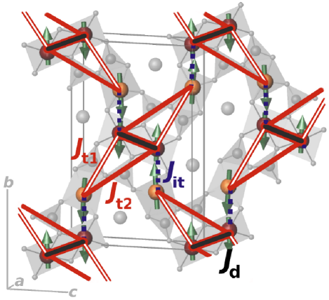
Figure 5: (Color online) Microscopic magnetic model for CdCu₂(BO₃)₂. The leading magnetic couplings are denoted by lines. The experimental magnetic structure (Ref. Hase et al., 2009) is depicted by arrows. The crystal structure sketch is the same as in Fig. 2.

In conclusion, DFT provides a robust qualitative microscopic magnetic model and unambiguously yields the signs of the leading $J_{i}$’s, as revealed by excellent agreement with the experimentally observed magnetic structure (Fig. 5). However, the accuracy of the individual magnetic couplings is not enough to provide a quantitative agreement with the experiments. In the next step, the evaluated model is refined by a simulation of its magnetic properties and subsequent comparison to the experiments.

IV.2 Simulations

Since the microscopic magnetic model is 2D and frustrated, numerically efficient techniques that account for the thermodynamic limit, such as quantum Monte Carlo (QMC) or density-matrix renormalization group (DMRG), can not be applied. Although new methods are presently under active development,[See; e.g.; ][]MERA; *PEPS a standard method to address such problems is exact diagonalization (ED) of the respective Hamiltonian matrix performed on finite lattices of $N$ spins.Richter et al. (2004a) However, the performance of present-day computational facilities limits the size of feasible finite lattices to $N$ = 24 sitesMisguich and Sindzingre (2007); *volb_DFT for finite-temperature properties or $N$ = 42 sitesRichter et al. (2004b); *kagome_GS_ED_N42_gap_AML for the GS. Additional restrictions arise from topological features of the particular model, e.g., only certain values of $N$ fit to periodic boundary conditions. Here, we apply ED to study the magnetic properties of CdCu₂(BO₃)₂ using exact diagonalization on $N$ = 16 sites (for the magnetic susceptibility) and $N$ = 32 sites (for GS spin-spin correlations and the GS magnetization process in magnetic field).

Due to the ambiguous choice of the DCC and $U_{3d}$, our DFT calculations do not provide a precise position of CdCu₂(BO₃)₂ in the parameter space of the proposed $J_{\text{d}}$–$J_{\text{t1}}$–$J_{\text{t2}}$–$J_{\text{it}}$ model. However, the ratios of the leading couplings (Table 1, three bottom lines) follow a distinct trend: the AMF solutions yield larger $J_{\text{t1}}$ : $J_{\text{d}}$ and substantially smaller $|J_{\text{it}}|$ : $J_{\text{d}}$ values, than FLL. Compared to the difference between the AMF and FLL solutions, the value of $U_{3d}$ and the functional used influence the ratios only slightly. Therefore, we adopt the two different DFT+$U$ solutions: the AMF solution $J_{\text{d}}$ : $J_{\text{t1}}$ : $J_{\text{t2}}$ : $J_{\text{it}}$ $\simeq$ 1 : 0.20 : 0.45 : $-$0.30 (AMF, $U_{3d}$ = 6.5 eV) and the FLL solution $J_{\text{d}}$ : $J_{\text{t1}}$ : $J_{\text{t2}}$ : $J_{\text{it}}$ $\simeq$ 1 : 0.15 : 0.25 : $-$0.70 (FLL, $U_{3d}$ = 9.5 eV) as starting points for simulations of magnetic susceptibility.

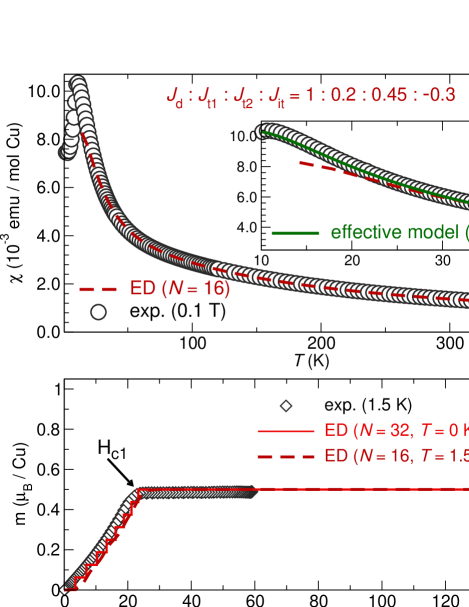
Figure 6: (Color online) Top panel: ED ($N$ = 16 sites) fit to the experimental (exp.) magnetic susceptibility. Deviations at $T$ $<$ 30 K are an extrinsic finite-size effect. Inset: fit to the low-temperature $\chi(T)$ using QMC for the effective model (Sec. V.1) on a $N$ =24$\times$24 sites finite lattice. Note the improved agreement between 15 and 30 K, compared to the ED fit. Bottom panel: magnetization curve measured at 1.5 K and simulated by ED (finite-temperature magnetization for $N$ = 16 and the GS magnetization for $N$ = 32 sites) scaled using the parameters ($J_{\text{d}}$ and $g$-factor) obtained from the fit to $\chi(T)$ (Table 2, top line).

We have simulated the magnetic susceptibility on a $N$ = 16 sites finite lattice (Fig. 12, bottom) with periodic boundary conditions, and by keeping the $J_{\text{d}}$ : $J_{\text{t1}}$ : $J_{\text{t2}}$ : $J_{\text{it}}$ ratios fixed. Such simulations yield the reduced magnetic susceptibility $\chi^{*}(T^{*})$, which can be compared to the experimental $\chi(T)$ by fitting free parameters: the overall energy scale $J_{\text{d}}$, the $g$-factor and the temperature-independent contribution $\chi_{0}$. In accord with the Mermin–Wagner theorem,Mermin and Wagner (1966) our 2D magnetic model does not account for long-range magnetic ordering, hence the simulated magnetic susceptibility is valid only for $T$ $>$ $T_{\text{N}}$ = 9.8 K.Hase et al. (2009) Moreover, at low temperatures (even above $T_{\text{N}}$) finite-size effects become relevant. To find an appropriate temperature range, we used an auxiliary eight-order high-temperature series expansion,Schmidt et al. (2011) and thus evaluated 30 K as a reasonable lowest fitting temperature for the $N$= 16 sites finite lattice.

The fitted values of $J_{\text{d}}$, $g$, and $\chi_{0}$ are summarized in Table 2. Since the FLL solution (Table 2, bottom line) yields unrealistically large $g$ = 2.457, it can be safely ruled out. By contrast, the AMF solution (Table 2, first row) yields a reasonable value of $g$ = 2.175.Janson et al. (2011); *Cu2V2O7_DFT; *Cu2As2O7 The resulting fit to the experimental $\chi(T)$ curve is shown in Fig. 6 (top).

Table 2: Fitted values of $J_{\text{d}}$ (in K), the $g$-factor and $\chi_{0}$ (in $10^{-4}\times$ emu $[$mol Cu$]^{-1}$), as well as the critical field $H_{\text{c}1}$ (in T), corresponding to the onset of a magnetization plateau. The simulations have been performed on $N$ = 16 sites finite lattices using ED.

$J_{\text{d}}$ : $J_{\text{t1}}$ : $J_{\text{t2}}$ : $J_{\text{it}}$	$J_{\text{d}}$	$g$	$\chi_{0}$	$H_{\text{c}1}$
1 : 0.20 : 0.45 : $-0.30$ (AMF)	178.0	2.175	0.9	24.1
1 : 0.15 : 0.25 : $-0.70$ (FLL)	291.9	2.457	$-$2.9	23.7

Next, we challenge the solutions from Table 2 using the high-field magnetization data (Fig. 6, bottom). In particular, the critical field $H_{\text{c}1}$, corresponding to the onset of the magnetization plateau (Fig. 6, bottom), can be estimated independently for both experimental and simulated curves. Experimentally, $H_{\text{c}1}$ = 23.2 T was evaluated by a pronounced minimum in $\partial^{2}m/\partial{}H^{2}$. The simulated magnetization curves $m(h^{*})$, where $h^{*}$ is the reduced magnetic field in the units of $J_{\text{d}}$, were scaled to the experimental data using the expression

$$H=\left(k_{\text{B}}\,J_{\text{d}}\,g^{-1}\,\mu_{\text{B}}^{-1}\right)h^{*},$$ (1)

and by adopting the values of $J_{\text{d}}$ and $g$ from the fits to $\chi(T)$. This way, $H_{\text{c}1}$ can be estimated directly, i.e., without using additional parameters beyond $J_{\text{d}}$ and $g$. Such $H_{\text{c}1}$ estimates are given in the last column of Table 2. Both the AMF and the FLL solutions are in excellent agreement with the experimental $H_{\text{c}1}$. Therefore, only the AMF solution $J_{\text{d}}$ : $J_{\text{t1}}$ : $J_{\text{t2}}$ : $J_{\text{it}}$ $\simeq$ 1 : 0.20 : 0.45 : $-$0.30 yields good agreement for both the $g$-factor and the $H_{\text{c}1}$ values. Thus, in the following, we restrict ourselves to the analysis of this solution (Table 2, first row).

So far, the simulations evidence a good agreement between the DFT-based model and the experimental information on thermodynamical properties. In the following, we perform an elaborate theoretical study of the proposed model. A deep insight into its physics enables further experimental verification of our microscopic scenario and allows to get prospects for new experiments.

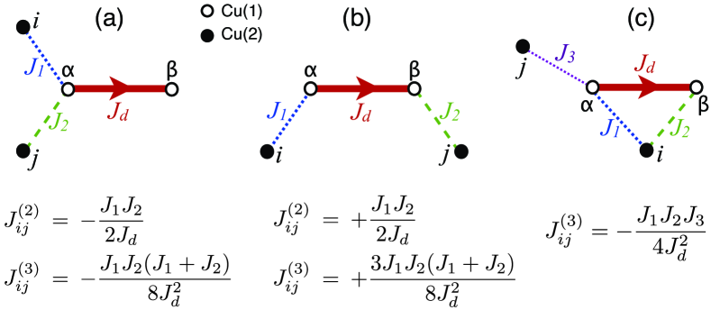
Figure 7: (Color online) The three topologically different clusters that contribute up to third order in the effective exchange $J_{ij}$ in the limit $J_{1,2,3}\!\ll\!J_{\text{d}}$, where $J_{1}$, $J_{2}$, and $J_{3}$ belong to the set: $J_{\text{t1}}$, $J_{\text{t2}}$, or $J_{\text{it}}$. Here $J_{ij}^{(2)}$ and $J_{ij}^{(3)}$ denote, respectively, the contributions from second and third-order perturbation theory. For any given cluster, we include only processes that involve each of the weak couplings at least once.

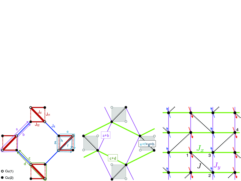
Figure 8: (Color online) The effective interactions between the Cu(2) sites (filled circles) up to lowest second order. Left panel: Eight paths $a-h$ that provide a nonzero exchange interaction up to second order. Middle panel: effective model based on $a$—$h$ paths: $J_{x}=c+d$, $J_{y}=a+b$, and $J=e+f+g+h$. In third order, one should also include the processes from the third cluster of Fig. 7, apart from a renormalization of the amplitudes $a$—$h$ (see text). Right panel: The resulting effective model in the topologically equivalent square lattice version of the structure. The indices 1-4 label the four sites of the unit cell of this lattice model. The arrows denote the classical GS of the model.

V Properties of the magnetic model

V.1 Effective low-energy theory

From the above discussion, it has become clear that the intradimer exchange $J_{\text{d}}$ is considerably larger than the remaining energy scales in the problem. This separation of energy scales leads naturally to the idea that the physics of the problem can be understood by a perturbative expansion around the limit $J_{\text{t1}}$ = $J_{\text{t2}}$ = $J_{\text{it}}$ = 0. In this limit, the Cu(1) sites coupled by $J_{\text{d}}$ form quantum-mechanical singlets, while the remaining, Cu(2) sites are free to point up or down, which defines a highly degenerate GS manifold. By turning on the remaining couplings $J_{\text{t1}}$, $J_{\text{t2}}$, and $J_{\text{it}}$, the Cu(2) sites begin to interact with each other through the virtual excitations of the Cu(1) dimers out of their singlet GS manifold. By integrating out these fluctuations, one can derive an effective low-energy model for the Cu(2) sites only. As we show below, a degenerate perturbation theory up to third order gives a remarkably accurate description of the low-energy physics of the problem.

Figure 7 shows the three topologically different clusters $G$ that involve a given Cu(1) dimer and contribute up to third order in perturbation theory. To avoid double counting of the processes that live on subclusters of $G$,Oitmaa et al. (2006) we keep only those processes that invoke each weak coupling of $G$ at least once. Here the weak couplings $J_{1,2,3}\!\ll\!J_{\text{d}}$ belong to the set: $J_{\text{t1}}$, $J_{\text{t2}}$, and $J_{\text{it}}$.

For the following discussion, it is essential to emphasize the difference between the first two clusters in Fig. 7: in (a) the two couplings involve the same site $\alpha$ of the dimer, while in (b) they involve both sites $\alpha$ and $\beta$. Since the singlet wave function $|s\rangle_{\alpha\beta}=\frac{1}{\sqrt{2}}\left(|\!\uparrow_{\alpha}\downarrow_{\beta}\rangle-|\!\downarrow_{\alpha}\uparrow_{\beta}\rangle\right)$ on the strong dimer is antisymmetric with respect to interchanging $\alpha$ and $\beta$, the two processes have opposite sign (and are equal in magnitude up to second order). In particular, if $J_{1}J_{2}>0$, the effective coupling between the sites $i$ and $j$ is ferromagnetic in (a) but antiferromagnetic in (b). For the third cluster, we have a third-order process where each of the three weak couplings $J_{1}$, $J_{2}$ and $J_{3}$ has been involved once in the whole process.

Using these quite general results, we may turn to our spin lattice and examine the possible effective processes that are active up to third order. We first discuss the contributions of the type shown in Fig. 7(a) and (b). Altogether, we find eight different paths $a$–$h$ $[$these are shown in Fig. 8(a)$]$ with the following amplitudes:

$$a=+\frac{J_{\text{t2}}J_{\text{it}}}{2J_{\text{d}}}\left(1+\frac{3(J_{\text{t2}}+J_{\text{it}})}{4J_{\text{d}}}\right)=-\frac{2403}{32000}J_{\text{d}},$$

$$b=-\frac{J_{\text{t1}}J_{\text{it}}}{2J_{\text{d}}}\left(1+\frac{J_{\text{t1}}+J_{\text{it}}}{4J_{\text{d}}}\right)=+\frac{117}{4000}J_{\text{d}},$$

$$c=-\frac{J_{\text{t2}}J_{\text{it}}}{2J_{\text{d}}}\left(1+\frac{J_{\text{t2}}+J_{\text{it}}}{4J_{\text{d}}}\right)=+\frac{2241}{32000}J_{\text{d}},$$

$$d=+\frac{J_{\text{t1}}J_{\text{it}}}{2J_{\text{d}}}\left(1+\frac{3(J_{\text{t1}}+J_{\text{it}})}{4J_{\text{d}}}\right)=-\frac{111}{4000}J_{\text{d}},$$

$$e=g=-\frac{J_{\text{t1}}J_{\text{t2}}}{2J_{\text{d}}}\left(1+\frac{J_{\text{t1}}+J_{\text{t2}}}{4J_{\text{d}}}\right)=-\frac{837}{16000}J_{\text{d}},$$

$$f=+\frac{J_{\text{t2}}^{2}}{2J_{\text{d}}}\left(1+\frac{3J_{\text{t2}}}{2J_{\text{d}}}\right)=\frac{5427}{32000}J_{\text{d}},$$

$$h=+\frac{J_{\text{t1}}^{2}}{2J_{\text{d}}}\left(1+\frac{3J_{\text{t1}}}{2J_{\text{d}}}\right)=\frac{13}{500}J_{\text{d}}~{}.$$

In the right-hand side equalities, we made use of the estimated ratios of the original couplings from Table 2 (the AMF solution). Including now the contributions of the type shown in Fig. 7(c), we get altogether three different effective exchange interactions between the Cu(2) spins:

$$J_{x}=c+d-\frac{J_{\text{t1}}J_{\text{t2}}J_{\text{it}}}{2J_{\text{d}}^{2}}\simeq+0.05578J_{\text{d}}~{},$$ (2)

$$J_{y}=a+b-\frac{J_{\text{t1}}J_{\text{t2}}J_{\text{it}}}{2J_{\text{d}}^{2}}\simeq-0.03234J_{\text{d}}~{},$$ (3)

$$J=e+f+g+h-\frac{J_{\text{t1}}J_{\text{t2}}(J_{\text{t1}}+J_{\text{t2}})}{2J_{\text{d}}^{2}}\simeq 0.06172J_{\text{d}}~{}.$$ (4)

These couplings are shown in the right panel of Fig. 8, where we use the square-lattice representation that is topologically equivalent to our effective model. Hence, the resulting effective model is the anisotropic Shastry-Sutherland lattice model with an AFM exchange coupling $J$ for the diagonal bonds, an AFM exchange $J_{x}$ for the horizontal bonds, and an FM exchange $J_{y}$ for the vertical bonds. This model readily explains the observed magnetic ordering on the Cu(2) sites since, on the classical level, one can minimize all interactions simultaneously in the collinear “stripe” configuration shown in the right panel of Fig. 8.

To challenge the applicability of the effective model, we refer again to the experimental $\chi(T)$ dependence. The nonfrustrated nature of the effective model enables us to use numerically efficient QMC techniques.Albuquerque et al. (2007) To this end, we have simulated $\chi^{*}(T^{*})$ of the effective model on a finite $N$ = 24$\times$24 sites lattice with periodic boundary conditions. A parameter-free fit to the experimental curve is obtained by using Eqs. (2)-(4) above, and the values of $J_{\text{d}}$ and $g$ from the ED fit (Table 2). By construction, the effective model is valid at low temperatures ($T$ $\ll$ $J_{\text{d}}$), but above the long-range magnetic ordering temperature $T_{N}$. In this temperature range, the effective model yields excellent agreement with the experimental $\chi(T)$ (see inset in top panel of Fig. 6), justifying it as an appropriate low-energy model for CdCu₂(BO₃)₂.

V.2 The size of the Cu(2) moments: linear spin wave theory in the effective model and QMC simulations

The size of the Cu(2) moment in the GS of the system is not equal to the classical value $g\mu_{B}/2$, but it will be somewhat lower due to quantum fluctuations. A similar correction is expected, e.g., for the GS energy. We can calculate these corrections by a standard $1/S$ semiclassical expansion around the stripe phase keeping only the quadratic portion of the fluctuations. The details of this calculation are provided in Appendix A, and here we only discuss the main results.

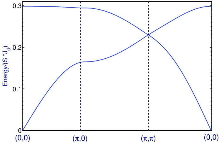
Figure 9: (Color online) Magnon dispersions (along certain symmetry directions in the BZ) obtained from linear spin wave theory around the stripe phase of the Cu(2) spins (see right panel of Fig. 8). There are four magnon branches but these pair up into two 2-fold degenerate branches, which is due to the symmetry of interchanging the sites (1,2) with (3,4) of the unit cell (see right panel of Fig. 8).

Figure 9 shows the magnon dispersions of the effective model along certain symmetry directions in the Brillouin zone (BZ). There are four magnon branches but these pair up into two 2-fold degenerate branches due to the symmetry of interchanging the sites (1,2) with (3,4) in the unit cell (see right panel of Fig. 8). The accuracy of the magnon dispersions was cross-checked by the McPhase code.Rotter (2004)

Let us now look at the quadratic correction to the GS energy which, as shown in Appendix A, consists of two terms, $\delta E_{1}$ and $\delta E_{2}$. The first term is given by $\delta E_{1}=-2\xi N_{uc}S$, where $\xi\equiv J+2J_{x}-2J_{y}$, and $N_{uc}$ is the number of unit cells. So adding $\delta E_{1}$ to the classical GS energy $E_{\text{class}}=-2\xi N_{uc}S^{2}$, amounts to a renormalization of the spin from $S$ to $\sqrt{S(S+1)}$. The second quadratic correction $\delta E_{2}$ stands for the zero-point energy of the final, decoupled harmonic oscillators of the theory $[$see Eq. (32)$]$, and can be calculated by a numerical integration over the BZ. Altogether, we find

$$E_{\text{class}}/N_{uc} = -0.119~{}J_{\text{d}}$$ (5)

$$\delta E_{1}/N_{uc} = -0.238~{}J_{\text{d}}$$ (6)

$$\delta E_{2}/N_{uc} \simeq +0.2092~{}J_{\text{d}}.$$ (7)

Thus, quadratic fluctuations actually reduce the GS energy by about $24\%$. We now turn to the renormalization of the magnetic moment, $\delta S$. As explained in Appendix A, this can also be calculated by a numerical integration over the BZ, see Eq. (35). We find

$$\delta S\simeq 0.159\Rightarrow S=0.5-\delta S\simeq 0.341~{}.$$ (8)

With $g\simeq 2.175$ we get a local magnetic moment on the Cu(2) sites of $m\simeq 0.742~{}\mu_{B}$, in line with the experimental value of $m\simeq 0.83~{}\mu_{B}$.Hase et al. (2009)

Since the model is not frustrated, we expect that the above prediction from linear spin wave theory is a good approximation. To verify this conjecture, we simulate the static structure factor $\mathbb{S}$ corresponding to the propagation vector of the collinear state ($\pi$,0) using QMC, which readily yields the order parameter $S$ $[$Eq. (33) in Ref. Sandvik, 1997$]$:

$$S^{2}(N)=\frac{3\mathbb{S}_{(\pi,0)}}{N}.$$ (9)

The results are presented in Fig. 10. We evaluated finite 2D lattices with up to $N$ = 48$\times$48 sites, and used Eq. (39b) from Ref. Sandvik, 1997 for the finite-size scaling (Fig. 10):

$$S^{2}(N)=S^{2}_{\infty}+\frac{\sigma_{1}}{\sqrt{N}}+\frac{\sigma_{2}}{N}+\frac{\sigma_{3}}{\sqrt{N}^{3}},$$ (10)

where $S_{\infty}$ is the magnetic moment, extrapolated to the thermodynamic limit. The resulting $S_{\infty}$ $\simeq$ 0.3297 yields $m$ = $g\mu_{B}S_{\infty}$ $\simeq$ 0.717 $\mu_{B}$, corroborating the linear spin-wave theory result.

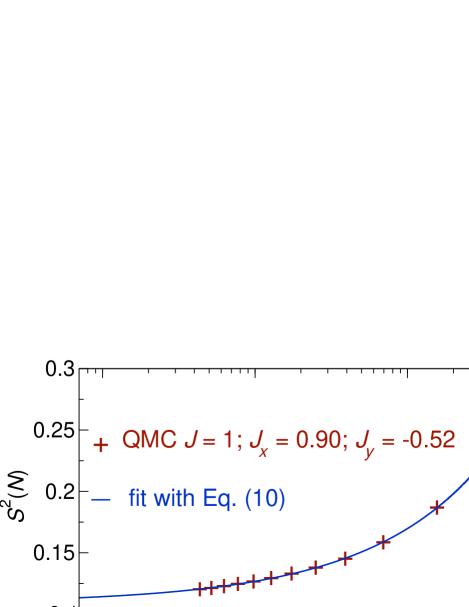
Figure 10: (Color online) Finite-size extrapolation of the quantity $S^{2}$($N$) defined in Eq. (9). Finite-$N$ values (crosses) were evaluated using QMC simulations for the effective model of the Cu(2) spins for a series of finite lattices up to $N$ = 48$\times$48 sites. The fit to Eq. (10) yields $\sigma_{1}$ = 0.5509, $\sigma_{2}$ = 0.6436, $\sigma_{3}$ = $-0.5097$, and $S_{\infty}$ $\simeq$ 0.3297, with the extrapolated magnetic moment $m$ = $g\mu_{B}S_{\infty}$ $\simeq$ 0.717 $\mu_{\text{B}}$.

V.3 Staggered polarization on the Cu(1) dimers

The effective low-energy theory derived above in Sec. V.1 is a theory for the projection of the full wave function of the system onto the manifold where all Cu(1) dimers form singlets. However, there is also a finite GS component out of this manifold. In particular, once the Cu(2) sites order magnetically in the collinear stripe phase (see right panel of Fig. 8), they will exert a finite exchange field on the Cu(1) dimers. A simple inspection of Fig. 11 tells us that this field is staggered, i.e., the local fields on the two Cu(1) spins of any given dimer are opposite to each other. Specifically, the fields $\mathbf{h}_{1,2}$, as shown in Fig. 11, are given by

$$\mathbf{h}_{1,2}\!=\!\pm\left(J_{\text{t1}}-J_{\text{t2}}+J_{\text{it}}\right)\!\langle\mathbf{S}_{\text{Cu}_{2}}\rangle=\mp 0.55J_{\text{d}}\langle\mathbf{S}_{\text{Cu}_{2}}\rangle,$$ (11)

where the last equation follows again from the DFT-based estimates for the ratios of the leading couplings (Table 2, first row).

Now, the important point is that the staggered field does not commute with the exchange interaction on the dimer, and as a result it can polarize the system immediately. This is very different from the case of a uniform field, where one must exceed the singlet-triplet gap $J_{\text{d}}$ in order to (uniformly) polarize the sites of the dimer.

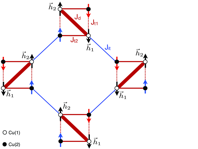
Figure 11: (Color online) The classical ground state of the effective model derived in Sec. V.1. The vectors $\mathbf{h}_{1,2}$ denote the local exchange fields on the Cu(1) sites exerted by the magnetically ordered Cu(2) sites (blue and red arrows).

To assess the amount of the induced polarization on the Cu(1) dimers, we consider a single AFM dimer with the exchange $J_{\text{d}}$ in the presence of a staggered field $h$, described by the Hamiltonian

$$\mathcal{H}=J_{\text{d}}~{}\mathbf{S}_{1}\cdot\mathbf{S}_{2}-h(S_{1}^{z}-S_{2}^{z})$$ (12)

The eigenstates of the dimer for $h=0$ are the singlet GS, $|s\rangle=\frac{1}{\sqrt{2}}\left(|\!\uparrow\downarrow\rangle-|\!\downarrow\uparrow\rangle\right)$, and the triplet excited states $|t_{1}\rangle=|\!\uparrow\uparrow\rangle$, $|t_{-1}\rangle=|\!\downarrow\downarrow\rangle$, and $|t_{0}\rangle=\frac{1}{\sqrt{2}}\left(|\!\uparrow\downarrow\rangle+|\!\downarrow\uparrow\rangle\right)$. The staggered field leaves $|t_{1}\rangle$ and $|t_{-1}\rangle$ intact, namely $\mathcal{H}|t_{\pm 1}\rangle=\frac{J}{4}|t_{\pm 1}\rangle$, but it mixes $|s\rangle$ with $|t_{0}\rangle$ as follows

$$\mathcal{H}|t_{0}\rangle=\frac{J_{\text{d}}}{4}|t_{0}\rangle-h|s\rangle$$ (13)

$$\mathcal{H}|s\rangle=-\frac{3J_{\text{d}}}{4}|s\rangle-h|t_{0}\rangle~{}.$$ (14)

A straightforward diagonalization of the Hamiltonian in the subspace of $\{|s\rangle,|t_{0}\rangle\}$ leads to the eigenvalues

$$E_{\pm}=-\frac{J_{\text{d}}}{4}\pm\sqrt{\left(\frac{J_{\text{d}}}{2}\right)^{2}+h^{2}}~{}.$$ (15)

For $h$ = 0, these results reduce to the energies $J_{\text{d}}/4$ and $-3J_{\text{d}}/4$ as expected. The GS is given by

$$|\psi_{-}\rangle=\frac{1}{N}\left[\left(J_{\text{d}}/2+\sqrt{J_{\text{d}}^{2}/4+h^{2}}\right)|s\rangle+h|t_{0}\rangle\right]~{},$$ (16)

where $N^{2}=2h^{2}+J_{\text{d}}^{2}/2+J_{\text{d}}\sqrt{J_{\text{d}}^{2}/4+h^{2}}$. As expected, $|\psi_{-}\rangle\!\mapsto\!|s\rangle$ for $h\!\mapsto\!0$, while for $h\gg J_{\text{d}}$, $|\psi_{-}\rangle\!\mapsto|\!\uparrow\downarrow\rangle$.

We may also look at the GS expectation value of the local polarizations on the dimer. We find

$$\langle\psi_{-}|S_{1,2}^{z}|\psi_{-}\rangle=\pm\frac{h(J_{\text{d}}/2+\sqrt{J_{\text{d}}^{2}/4+h^{2}})}{2h^{2}+J_{\text{d}}^{2}/2+J_{\text{d}}\sqrt{J_{\text{d}}^{2}/4+h^{2}}}~{}.$$ (17)

For $h=0$ we recover $\langle\psi_{-}|S_{1,2}^{z}|\psi_{-}\rangle=0$, while for $h\gg J_{\text{d}}$ we get maximum polarizations $\langle\psi_{-}|S_{1,2}^{z}|\psi_{-}\rangle\mapsto\pm 1/2$, which corresponds to the state $|\!\!\uparrow\downarrow\rangle$. In the linear response regime $h\!\!\ll\!\!J_{\text{d}}$, we get $\langle\psi_{-}|S_{1,2}^{z}|\psi_{-}\rangle\simeq\pm h/J_{\text{d}}$, thus the staggered susceptibility is $\chi_{s}=1/J_{\text{d}}$.

We can now apply these results to our case. Using Eqs. (11) and (17), the polarization on the Cu(1) sites can be estimated as

$$|\langle S_{\text{Cu}_{1}}\rangle|\simeq 0.176\simeq 0.516|\langle S_{\text{Cu}_{2}}\rangle|~{},$$ (18)

which is again in very good agreement with the experimental $|\langle S_{\text{Cu}_{1}}\rangle|$ = 0.54$|\langle S_{\text{Cu}_{2}}\rangle|$ from Ref. Hase et al., 2009.

V.4 The 1/2-plateau phase and the critical field $H_{c1}$

The separation of energy scales in CdCu₂(BO₃)₂ is a natural reason for the formation of the 1/2 magnetization plateau. Due to the strong $J_{\text{d}}$, the Cu(1) spins involved in the $J_{\text{d}}$-dimers are much harder to polarize with a uniform field than the weakly coupled Cu(2) spins. Naturally then, the 1/2-plateau corresponds to the state with the Cu(2) spins fully polarized and the Cu(1) dimers still carrying a strong singlet amplitude and a finite staggered polarization.

Here, we go one step further and calculate $H_{c1}$, the onset field of the 1/2-plateau by considering the one-magnon spectrum of the effective model in the fully polarized phase. The one-magnon space consists of states with all but one spins pointing up. We label the possible positions of the down spin by one index for the unit cell and another index $\alpha=1-4$ which specifies one of the 4 inequivalent Cu sites within the unit cell (see sites 1-4 in the right panel of Fig. 8). A straightforward Fourier transform gives the following $4\times 4$ Hamiltonian matrix in the one-magnon space

$$\delta\mathcal{H}_{\text{1-magnon}}(\mathbf{k})=\frac{1}{2}\left(\begin{array}[]{c c c c}2\lambda&J&J_{x}(1+e^{-ik_{x}})&J_{y}(e^{-ik_{x}}+e^{-i(k_{x}+k_{y})})\\ J&2\lambda&J_{y}(1+e^{-ik_{y}})&J_{x}(e^{-ik_{y}}+e^{-i(k_{x}+k_{y})})\\ J_{x}(1+e^{ik_{x}})&J_{y}(1+e^{ik_{y}})&2\lambda&J\\ J_{y}(e^{ik_{x}}+e^{i(k_{x}+k_{y})})&J_{x}(e^{ik_{y}}+e^{i(k_{x}+k_{y})})&J&2\lambda\end{array}\right)~{},$$

where we measure all energies relative to the energy of the fully polarized state, and $\lambda=g\mu_{B}H-\left(J_{x}+J_{y}+J/2\right)$. Using Eqs. (2)-(4), we find that one of the four branches of the one-magnon spectrum becomes soft (reaches zero energy) at $\mathbf{k}=0$ when $g\mu_{B}H=J+2J_{x}=\frac{1109}{6400}J_{\text{d}}$. This soft mode signals the instability of the fully polarized state, hence

$$H_{c1}=\frac{1109}{6400}\frac{J_{\text{d}}}{g\mu_{B}}~{}.$$ (19)

With $g$ $\simeq$ 2.175 and $J_{\text{d}}$ = 178 K (AMF solution from Table 2), we obtain $H_{c1}$ $\simeq$ 21.11 T, which is in very good agreement with the experimental value of $H_{c1}$ = 23.2 T. This confirms that the third-order perturbation theory gives an adequate quantitative description of the low-energy physics. It also confirms that our set of exchange parameters gives an accurate quantitative description of the magnetism in this compound.

V.5 Exact Diagonalizations

We are now going to check the above physical picture obtained from the effective model by numerical exact diagonalizations on the original model. We first address the nature of the magnetic GS by evaluating the spin-spin correlations $\langle{}\bf{S}_{0}\!\cdot\!\bf{S}_{\text{R}}\rangle$ as a function of the “distance” R (Fig. 12). In order to elucidate the difference in the coupling regimes of Cu(1) and Cu(2) spins, we choose two independent paths on the 2D spin lattice, with different initial spins $\bf{S}_{0}$ (Fig. 12, lower panel). As expected for strong $J_{\text{d}}$, the structural dimers exhibit strong AFM correlation $\langle{}\bf{S}_{0}\!\cdot\!\bf{S}_{\text{1}}\rangle$ = $-0.57$ (green line in Fig. 12), while the $J_{\text{it}}$ bonds bear much weaker FM correlation $\langle{}\bf{S}_{0}\cdot\bf{S}_{\text{1}}\rangle$ = $0.15$ (brown line in Fig. 12).

A rough estimate for the ordered magnetic moment can be obtained from the spin correlations of the maximally separated spins on a finite lattice. The small size of the 32-site finite lattice impedes a direct evaluation of the order parameters. However, the same-sublattice correlations for the Cu(1) and Cu(2) sublattices, evaluated using the same $N$ = 32 cluster, can be compared to each other. In this way, finite size effects, which are crucial for the values of $m_{\text{Cu(1)}}$ and $m_{\text{Cu(2)}}$, should be largely remedied for the $m_{\text{Cu(1)}}$:$m_{\text{Cu(2)}}$ ratio.

The maximal separation in terms of exchange bonds between the same-sublattice spins on the 32-site finite lattice is five and corresponds to $\langle{}\bf{S}_{0}\!\cdot\!\bf{S}_{8}\rangle$ correlations in Fig. 12. ED yields $\langle{}\bf{S}_{0}\!\cdot\!\bf{S}_{8}\rangle[\text{Cu(1)}]$ = 0.060 and $\langle{}\bf{S}_{0}\!\cdot\!\bf{S}_{8}\rangle[\text{Cu(2)}]$ = 0.174 for Cu(1) and Cu(2), respectively. In the simplest picture, the quantity $\sqrt{\langle{}\bf{S}_{0}\!\cdot\!\bf{S}_{8}\rangle}[\text{Cu(1)}]$ : $\sqrt{\langle{}\bf{S}_{0}\!\cdot\!\bf{S}_{8}\rangle}[\text{Cu(2)}]$ = 0.59 should be close to the ratio of the magnetic moments. Although the results may be still affected by finite-size effects, a comparison to the experimentalHase et al. (2009) $m_{\text{Cu(1)}}$ : $m_{\text{Cu(2)}}$ = 0.45 : 0.83 = 0.54 reveals surprisingly good agreement between theory and experiment.

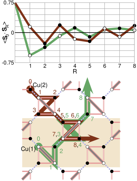
Figure 12: (Color online) Upper panel: spin correlations $\langle{}\mathbf{S}_{0}\cdot\mathbf{S}_{\text{R}}\rangle$ in the magnetic ground state of CdCu₂(BO₃)₂, simulated on the 32-site finite lattice with periodic boundary conditions using ED. Lower panel: $N$ = 32 sites (full plot) and $N$ = 16 sites (shaded rectangle) finite lattices used in our ED. $\mathbf{S}_{0}$–$\mathbf{S}_{\text{R}}$ pathways are used for the $\langle{}\mathbf{S}_{0}\!\cdot\!\mathbf{S}_{\text{R}}\rangle$(R) plot in the upper panel. For the notation of exchange couplings, see Fig. 5.

Next, we examine the evolution of the GS expectation values of the local spin-spin correlations in magnetic field, which are presented in Fig. 13. For $h^{*}$ = 0, the correlations within the structural dimers and along the $J_{\text{t2}}$ bonds are dominant, amounting to $-$0.570 and $-$0.366, respectively. The first one is somewhat weaker than the pure singlet value of $-$0.75, because of the finite admixture with the triplet $|t_{0}\rangle$ in GS, as explained in Sec. V.3.

Now, according to Fig. 13, a magnetic field enhances the intradimer correlation. This counter-intuitive result can be physically understood as follows. In a finite field, the Cu(2) spins order in the plane perpendicular to the field (this happens in an infinitesimal field, since the crystalline anisotropy effects are neglected) and at the same time develop a uniform component along the field. While the former, as discussed in Sec. V.3, gives rise to a staggered exchange field on the Cu(1) dimers, the latter induces a uniform exchange field. By increasing the external field, the staggered component decreases, while the uniform component increases. At the 1/2-plateau, the Cu(2) spins are almost fully polarized, hence only the uniform component survives. Now, in contrast to the staggered component, the uniform field commutes with the exchange interaction on the Cu(1) dimer and thus leaves the singlet GS wave function intact. In other words, the magnetic field suppresses the admixture of a triplet in the singlet GS. The steep decrease in the correlation along the $J_{\text{t2}}$ bonds in a field reflects the same physics.

At the critical field $h^{*}$ $\simeq$ 0.2 (24 T), CdCu₂(BO₃)₂ enters the 1/2-plateau phase. Here, in contrast with the strong AFM correlations within the Cu(1) dimers ($\langle{}\bf{S}_{0}\!\cdot\!\bf{S}_{\text{1}}\rangle$ = $-$0.718), the correlations along the $J_{\text{t1}}$, $J_{\text{t2}}$ and $J_{\text{it}}$ bonds are much smaller and similar in size, but have different signs. The negative correlation for $J_{\text{t2}}$ and the positive for $J_{\text{it}}$ are in accord with the nature of these two couplings, AFM and FM, respectively. For weaker AFM $J_{\text{t1}}$, the correlation is positive due to the frustrated nature of the spin model.

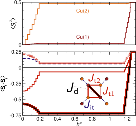
Figure 13: (Color online) Magnetization $\langle{}S^{z}_{i}\rangle$ for Cu(1) and Cu(2) spins, as well as spin correlations $\langle{}\mathbf{S}_{i}\cdot\mathbf{S}_{j}\rangle$ corresponding to the leading couplings $J_{\text{d}}$, $J_{\text{t1}}$, $J_{\text{t2}}$, and $J_{\text{it}}$ (line styles according to the inset) as a function of magnetic field $h^{*}$ in units of $J_{\text{d}}$.

Since the local spin correlation on the Cu(1) dimers is very close to the singlet value, the contribution to the total magnetization from the Cu(1) spins is expected to be negligible. Therefore, the magnetization results predominantly from the Cu(2) spins. This picture is supported by simulations of the local magnetizations $\langle{}S^{z}_{i}\rangle$, shown in the upper panel of Fig. 13. In the 1/2-plateau phase, the local magnetization of Cu(2) is $\langle{}S^{z}_{\text{Cu2}}\rangle$ = 0.483, while the magnetization of Cu(1) is negligibly small with $\langle{}S^{z}_{\text{Cu1}}\rangle$ = 0.017, which also agrees with the main picture obtained from the effective model. Therefore, within the error from finite-size effects, only about 3 % of the Cu(1) moments are polarized in the 1/2-plateau phase.

Let us now discuss the width of the 1/2-plateau. This corresponds to the energy we need to pay to fully polarize a Cu(1) dimer, i.e. to convert a singlet into a triplet excitation. The width of the plateau can be estimated by neglecting the perturbative corrections that give rise to a hopping of these triplet excitations (and, thus, to a small dispersion). Our ED results (upper panel of Fig. 13) agree very well with this estimate: the critical field at which the 1/2-plateau ends is $h^{*}$ = 1.17 (143 T).

Now, once we pay the energy $J_{\text{d}}$ to excite a triplet, we can also polarize the remaining Cu(1) dimers very quickly due to the small (perturbative) kinetic energy scale of the triplet excitations. Indeed, our ED results for the magnetization above $H_{c2}$ show a rapid increase up to the saturation value. In addition, we find no indication for any other magnetization plateaux above 1/2, which suggests that the interaction between the triplet excitations is negligible.

VI Summary and outlook

The magnetism of CdCu₂(BO₃)₂ was investigated on a microscopic level by using extensive DFT band structure calculations, ED and QMC simulations, third-order perturbation theory, as well as high-field magnetization measurements. In contrast to the previously suggested “chains + dimers” model, we evaluate a quasi-2D magnetic model with mostly antiferromagnetic couplings: an intradimer exchange $J_{\text{d}}$ and two intra-tetramer interactions $J_{\text{t1}}$ and $J_{\text{t2}}$, as well as a ferromagnetic coupling $J_{\text{it}}$ between the tetramers. The $J_{\text{d}}$ : $J_{\text{t1}}$ : $J_{\text{t2}}$ : $J_{\text{it}}$ ratio is close to 1 : 0.20 : 0.45 : $-0.30$ with a dominant $J_{\text{d}}$ of about 178 K. Topologically, this microscopic model can be regarded as decorated anisotropic Shastry-Sutherland lattice (Fig. 1).

While the spin pairs forming the structural dimers show a clear tendency to form magnetic singlets on the $J_{\text{d}}$ bonds, the low-temperature magnetic properties of CdCu₂(BO₃)₂ are governed by interdimer couplings. In contrast to the strongly frustrated SrCu₂(BO₃)₂ featuring a singlet ground state, the inequivalence of $J_{\text{t1}}$ and $J_{\text{t2}}$ largely lifts the frustration and triggers long-range antiferromagnetic ordering. This model correctly reproduces the substantial difference between Cu(1) and Cu(2) ordered moments, as observed experimentally. Our simulations and the subsequent fitting of the magnetic susceptibility and magnetization further support the microscopic model and the proposed parameterization.

It is interesting to compare the key results for CdCu₂(BO₃)₂ with the archetype Shastry-Sutherland $S$ = $\frac{1}{2}$ system SrCu₂(BO₃)₂. Although the substitution of Sr by Cd significantly alters the crystal structure and stabilizes a different magnetic ground state, the microscopic magnetic models of both systems bear apparent similarities (Fig. 1). Moreover, the dominance of the $J_{\text{d}}$ coupling in CdCu₂(BO₃)₂ leads to an effective nonfrustrated model for the Cu(2) spins, which is topologically equivalent to an anisotropic Shastry-Sutherland lattice model. It is noteworthy that the phase diagram of such a model was recently discussed.Furukawa et al. (2011)

One of the main objectives of this study is to stimulate further experimental activity on CdCu₂(BO₃)₂. Such studies are necessary to refine the parameters of the suggested microscopic model and address yet unresolved issues. Our extensive analysis of the magnetic properties of this complex system delivers several results that should be challenged experimentally. For example, we have resolved that the Cu(1) dimers develop a sizable staggered polarization which is suppressed by an applied field and vanishes at the 1/2 plateau. This behavior could be addressed experimentally by nuclear magnetic resonance.[See; e.g.][]SCBO_NMR_stagger; *SCBO_NMR_stagger_DM On the other hand, inelastic neutron scattering experiments could challenge the magnon dispersions calculated for the effective low-energy model. In addition, the magnetic couplings, associated with edge-sharing and corner-sharing connections of CuO₄ plaquettes, are strongly dependent on Cu–O–Cu angles. Therefore, the magnetic properties of CdCu₂(BO₃)₂ could be tuned by applying external pressure. Similar experiments on SrCu₂(BO₃)₂ (Ref. Waki et al., 2007) reveal excellent potential of such studies.

Appendix A Linear spin wave theory around the stripe phase of the effective model

Here, we provide the details of the linear spin wave theory around the stripe phase of the Cu(2) spins. We begin with the effective model Hamiltonian that was derived in Sec. V.1 for the Cu(2) spins:

$$\mathcal{H} \!=\! \sum_{u}J~{}\Big{(}\mathbf{S}_{1,u}\cdot\mathbf{S}_{2,u}+\mathbf{S}_{3,u}\cdot\mathbf{S}_{4,u}\Big{)}$$ (20)

$$+ J_{x}~{}\mathbf{S}_{3,u}\cdot\Big{(}\mathbf{S}_{1,u}+\mathbf{S}_{1,u+t_{x}}\Big{)}$$

$$+ J_{y}~{}\mathbf{S}_{3,u}\cdot\Big{(}\mathbf{S}_{2,u}+\mathbf{S}_{2,u+t_{y}}\Big{)}$$

$$+ J_{x}~{}\mathbf{S}_{4,u}\cdot\mathbf{S}_{2,u+t_{y}}+J_{x}~{}\mathbf{S}_{2,u}\cdot\mathbf{S}_{4,u-t_{x}-t_{y}}$$

$$+ J_{y}~{}\mathbf{S}_{1,u}\cdot\mathbf{S}_{4,u-t_{x}-t_{y}}+J_{y}~{}\mathbf{S}_{4,u}\cdot\mathbf{S}_{1,u+t_{x}}$$

where $\mathbf{t}_{x,y}=2a~{}\mathbf{e}_{x,y}$ are the primitive translation vectors in the model ($a$ is the lattice constant of the square lattice), and the index $u$ labels the unit cell. The remaining spin operator index (1-4) labels the 4 sites of the unit cell (see right panel of Fig. 8). We then take as our reference classical state the one where the spins 1 and 3 (resp. 2 and 4) of the unit cell point along the positive (resp. negative) $z$-axis, and perform a standard Holstein-Primakoff expansion in terms of four bosonic operators labeled as $a_{u},b_{u},c_{u},d_{u}$, which correspond to the four spins per unit cell $S_{1,u},S_{2,u},S_{3,u},S_{4,u}$ respectively. The transformation reads

$$S_{1,u}^{z}\simeq-S+a_{u}^{+}a_{u},~{}~{}~{}S_{1,u}^{+}\simeq\sqrt{2S}~{}a_{u}^{+}$$

$$S_{2,u}^{z}\simeq S-b_{u}^{+}b_{u},~{}~{}~{}S_{2,u}^{+}\simeq\sqrt{2S}~{}b_{u}$$

$$S_{3,u}^{z}\simeq S-c_{u}^{+}c_{u},~{}~{}~{}S_{3,u}^{+}\simeq\sqrt{2S}~{}c_{u}$$

$$S_{4,u}^{z}\simeq-S+d_{u}^{+}d_{u},~{}~{}~{}S_{4,u}^{+}\simeq\sqrt{2S}~{}d_{u}^{+}~{}.$$ (21)

Replacing these expressions in the Hamiltonian and performing a Fourier transform, we get

$$\mathcal{H}=E_{0b}+\mathcal{H}_{2b}+\mathcal{O}(S^{0})$$ (22)

where $E_{ob}=-2\xi N_{uc}S^{2}$ stands for the classical energy, and $\xi\equiv J+2J_{x}-2J_{y}$. The term $\mathcal{H}_{2b}$ stands for the quadratic Hamiltonian which can be written in the compact matrix form

$$\mathcal{H}_{2b}=\delta E_{1}+\frac{S}{2}\sum_{k}\mathbf{A}_{k}^{+}\cdot\mathbf{M}_{k}\cdot\mathbf{A}_{k}$$ (23)

where $\delta E_{1}=-2\xi N_{uc}S$,

$$\mathbf{A}_{k}^{+}\!=\!\left(\begin{array}[]{cccccccc}a_{k}^{+},&b_{k}^{+},&c_{k}^{+},&d_{k}^{+},&a_{-k},&b_{-k},&c_{-k},&d_{-k}\end{array}\right),$$ (24)

$$\mathbf{M}_{k}=\left(\begin{array}[]{cc}\mathbf{C}_{k}&\mathbf{D}_{k}\\ \mathbf{D}_{k}&\mathbf{C}_{k}\end{array}\right)~{},$$ (25)

and

$$\mathbf{C}_{k}=\left(\begin{array}[]{cccc}\xi&0&0&J_{y}e^{-ik_{x}}(1+e^{-ik_{y}})\\ &&&\\ 0&\xi&J_{y}(1+e^{-ik_{y}})&0\\ &&&\\ 0&J_{y}(1+e^{ik_{y}})&\xi&0\\ &&&\\ J_{y}e^{ik_{x}}(1+e^{ik_{y}})&0&0&\xi\end{array}\right)~{},$$ (26)

$$\mathbf{D}_{k}=\left(\begin{array}[]{cccc}0&-J&-J_{x}(1+e^{-ik_{x}})&0\\ &&&\\ -J&0&0&-J_{x}e^{-ik_{y}}(1+e^{-ik_{x}})\\ &&&\\ -J_{x}(1+e^{ik_{x}})&0&0&-J\\ &&&\\ 0&-J_{x}e^{ik_{y}}(1+e^{ik_{x}})&-J&0\\ \end{array}\right)~{}.$$ (27)

To diagonalize $\mathcal{H}_{2b}$ we search for a new set of bosonic operators $\tilde{\mathbf{A}}_{k}$ given by the generalized Bogoliubov transformation $\mathbf{A}_{k}=\mathbf{S}_{k}\cdot\tilde{\mathbf{A}}_{k}$, such that the matrix $\mathbf{S}_{k}^{+}\mathbf{M}_{k}\mathbf{S}_{k}\equiv\mathbf{\Omega}_{k}$ becomes diagonal. The transformation must also preserve the bosonic commutation relations, which can be expressed compactly as $\mathbf{g}=\tilde{\mathbf{g}}=\mathbf{S}_{k}\cdot\mathbf{g}\cdot\mathbf{S}_{k}^{+}$, where $\mathbf{g}$ is the “commutator” matrix

$$\mathbf{g}=\mathbf{A}_{k}\cdot\mathbf{A}_{k}^{+}-\left(\left(\mathbf{A}_{k}^{+}\right)^{T}\cdot\mathbf{A}_{k}^{T}\right)^{T}=\left(\begin{array}[]{cc}{\bf 1}_{4}&0\\ 0&-{\bf 1}_{4}\end{array}\right)$$ (28)

and ${\bf 1}_{4}$ stands for the $4\times 4$ identity matrix. The above two conditions give

$$(\mathbf{g}\mathbf{M}_{k})\cdot\mathbf{S}_{k}=\mathbf{S}_{k}\cdot\left(\mathbf{g}\mathbf{\Omega}_{k}\right)\equiv\mathbf{S}_{k}\cdot\mathbf{\Omega}^{\prime}_{k}$$ (29)

which is an eigenvalue equation in matrix form (the columns of $\mathbf{S}_{k}$ contain the eigenvectors of $\mathbf{g}\mathbf{M}_{k}$).

One can showBlaizot and Ripka (1985) that if $\mathbf{M}_{k}$ is semi-definite positive, then the eigenvalues of $\mathbf{gM}_{k}$ come in opposite pairs:

$$\mathbf{\Omega}^{\prime}_{k}=\left(\begin{array}[]{cc}\boldsymbol{\omega}_{k}&0\\ 0&-\boldsymbol{\omega}_{k}\end{array}\right)\Rightarrow\mathbf{\Omega}_{k}=\left(\begin{array}[]{cc}\boldsymbol{\omega}_{k}&0\\ 0&\boldsymbol{\omega}_{k}\end{array}\right)$$ (30)

where $\boldsymbol{\omega}_{k}$ is a diagonal matrix with non-negative entries $\omega_{1k},\!\ldots\!,\omega_{4k}$. This in turn leads to

$$\mathcal{H}_{2b}=\delta E_{1}+\delta E_{2}+S\sum_{k}\left(\omega_{1k}~{}\tilde{a}_{k}^{+}\tilde{a}_{k}+\!\ldots\!+\omega_{4k}~{}\tilde{d}_{k}^{+}\tilde{d}_{k}\right)~{},$$ (31)

where the second correction

$$\delta E_{2}=\frac{S}{2}\sum_{k}\left(\omega_{1k}+\!\ldots\!+\omega_{4k}\right)~{},$$ (32)

stands for the total contribution from the zero-point energy of all independent harmonic operators involved in the theory.

A.1 Renormalization of the magnetic moments

Let us now look at the effect of the quadratic fluctuations on the magnetic moments. We consider the spin $\mathbf{S}_{1}$ operator inside the unit cell $n=0$. The classical vector points along the $z$-axis. We have

$$\mathbf{S}_{1}^{z}=S-a_{n=0}^{+}a_{n=0}=S-\frac{1}{N_{uc}}\sum_{k,q}a_{k}^{+}a_{q}~{}.$$ (33)

Using the transformation $\mathbf{A}_{k}=\mathbf{S}_{k}\cdot\tilde{\mathbf{A}}_{k}$, we get

$$\mathbf{S}_{1}^{z}\!=\!S-\frac{1}{N_{uc}}\sum_{k,q}\sum_{ij}S_{k}(1,i)^{\ast}S_{q}(1,j)~{}\tilde{A}_{k}^{+}(i)\tilde{A}_{k}(j)~{}.$$ (34)

In the vacuum GS, the only non-vanishing expectation values are of the type $\langle\tilde{a}_{k}\tilde{a}_{k}^{+}\rangle=1$. Thus from the above sum we should keep only terms with $i\!=\!j\!=\!5-8$ and $k\!=\!q$, namely

$$\langle\mathbf{S}_{1}^{z}\rangle=S-\frac{1}{N_{uc}}\sum_{k}\sum_{i=5}^{8}|S_{k}(1,i)|^{2}~{}.$$ (35)

The second term can be calculated by a numerical integration over the BZ.

References

- Majumdar and Ghosh (1969a) C. K. Majumdar and D. K. Ghosh, J. Math. Phys. 10, 1388 (1969a).
- Majumdar and Ghosh (1969b) C. K. Majumdar and D. K. Ghosh, J. Math. Phys. 10, 1399 (1969b).
- Kitaev (2006) A. Kitaev, Ann. Phys. 321, 2 (2006), cond-mat/0506438 .
- Shastry and Sutherland (1981) B. S. Shastry and B. Sutherland, Physica B+C 108, 1069 (1981).
- Miyahara and Ueda (1999) S. Miyahara and K. Ueda, Phys. Rev. Lett. 82, 3701 (1999), cond-mat/9807075 .
- Kageyama et al. (1999) H. Kageyama, K. Yoshimura, R. Stern, N. V. Mushnikov, K. Onizuka, M. Kato, K. Kosuge, C. P. Slichter, T. Goto, and Y. Ueda, Phys. Rev. Lett. 82, 3168 (1999).
- Onizuka et al. (2000) K. Onizuka, H. Kageyama, Y. Narumi, K. Kindo, Y. Ueda, and T. Goto, J. Phys. Soc. Jpn. 69, 1016 (2000).
- Vecchini et al. (2009) C. Vecchini, O. Adamopoulos, L. Chapon, A. Lappas, H. Kageyama, Y. Ueda, and A. Zorko, J. Solid State Chem. 182, 3275 (2009).
- Miyahara and Ueda (2000) S. Miyahara and K. Ueda, J. Phys. Soc. Jpn. (Suppl. B) 69, 72 (2000), cond-mat/0004260 .
- Miyahara and Ueda (2003) S. Miyahara and K. Ueda, J. Phys.: Condens. Matter 15, R327 (2003).
- Koga and Kawakami (2000) A. Koga and N. Kawakami, Phys. Rev. Lett. 84, 4461 (2000), cond-mat/0003435 .
- Darradi et al. (2005) R. Darradi, J. Richter, and D. J. J. Farnell, Phys. Rev. B 72, 104425 (2005), cond-mat/0504283 .
- Waki et al. (2007) T. Waki, K. Arai, M. Takigawa, Y. Saiga, Y. Uwatoko, H. Kageyama, and Y. Ueda, J. Phys. Soc. Jpn. 76, 073710 (2007), arXiv:0706.0112 .
- Takigawa et al. (2010) M. Takigawa, T. Waki, M. Horvatić, and C. Berthier, J. Phys. Soc. Jpn. 79, 011005 (2010).
- Moliner et al. (2011) M. Moliner, I. Rousochatzakis, and F. Mila, Phys. Rev. B 83, 140414 (2011), arXiv:1012.5177 .
- Ivanov and Richter (1997) N. B. Ivanov and J. Richter, Phys. Lett. A 232, 308 (1997), cond-mat/9705162 .
- Belik et al. (2004) A. A. Belik, M. Azuma, and M. Takano, J. Solid State Chem. 177, 883 (2004).
- Johannes et al. (2006) M. D. Johannes, J. Richter, S.-L. Drechsler, and H. Rosner, Phys. Rev. B 74, 174435 (2006), cond-mat/0609430 .
- Tsirlin and Rosner (2009) A. A. Tsirlin and H. Rosner, Phys. Rev. B 79, 214417 (2009), arXiv:0901.4498 .
- Colman et al. (2008) R. H. Colman, C. Ritter, and A. S. Wills, Chem. Mater. 20, 6897 (2008), arXiv:0811.4048 .
- Janson et al. (2008) O. Janson, J. Richter, and H. Rosner, Phys. Rev. Lett. 101, 106403 (2008), arXiv:0806.1592 .
- Colman et al. (2010) R. H. Colman, A. Sinclair, and A. S. Wills, Chem. Mater. 22, 5774 (2010).
- Janson et al. (2011) O. Janson, A. A. Tsirlin, J. Sichelschmidt, Y. Skourski, F. Weickert, and H. Rosner, Phys. Rev. B 83, 094435 (2011), arXiv:1011.5393 .
- Tsirlin et al. (2010) A. A. Tsirlin, O. Janson, and H. Rosner, Phys. Rev. B 82, 144416 (2010), arXiv:1007.1646 .
- Arango et al. (2011) Y. C. Arango, E. Vavilova, M. Abdel-Hafiez, O. Janson, A. A. Tsirlin, H. Rosner, S.-L. Drechsler, M. Weil, G. Nénert, R. Klingeler, O. Volkova, A. Vasiliev, V. Kataev, and B. Büchner, Phys. Rev. B 84, 134430 (2011), arXiv:1110.0447 .
- Janson et al. (2009) O. Janson, W. Schnelle, M. Schmidt, Y. Prots, S.-L. Drechsler, S. K. Filatov, and H. Rosner, New J. Phys. 11, 113034 (2009), arXiv:0907.4874 .
- Deisenhofer et al. (2006) J. Deisenhofer, R. M. Eremina, A. Pimenov, T. Gavrilova, H. Berger, M. Johnsson, P. Lemmens, H.-A. Krug von Nidda, A. Loidl, K.-S. Lee, and M.-H. Whangbo, Phys. Rev. B 74, 174421 (2006), cond-mat/0610458 .
- Das et al. (2008) H. Das, T. Saha-Dasgupta, C. Gros, and R. Valentí, Phys. Rev. B 77, 224437 (2008), cond-mat/0703675 .
- Pickett (1989) W. E. Pickett, Rev. Mod. Phys. 61, 433 (1989).
- Janson et al. (2007) O. Janson, R. O. Kuzian, S.-L. Drechsler, and H. Rosner, Phys. Rev. B 76, 115119 (2007).
- Choi et al. (2003) K.-Y. Choi, Y. G. Pashkevich, K. V. Lamonova, H. Kageyama, Y. Ueda, and P. Lemmens, Phys. Rev. B 68, 104418 (2003).
- Liu et al. (2005) G. T. Liu, J. L. Luo, N. L. Wang, X. N. Jing, D. Jin, T. Xiang, and Z. H. Wu, Phys. Rev. B 71, 014441 (2005), cond-mat/0406306 .
- Liu et al. (2006) G. T. Liu, J. L. Luo, Y. Q. Guo, S. K. Su, P. Zheng, N. L. Wang, D. Jin, and T. Xiang, Phys. Rev. B 73, 014414 (2006), cond-mat/0512521 .
- Haravifard et al. (2006) S. Haravifard, S. R. Dunsiger, S. El Shawish, B. D. Gaulin, H. A. Dabkowska, M. T. F. Telling, T. G. Perring, and J. Bonča, Phys. Rev. Lett. 97, 247206 (2006), cond-mat/0608442 .
- Hase et al. (2005) M. Hase, M. Kohno, H. Kitazawa, O. Suzuki, K. Ozawa, G. Kido, M. Imai, and X. Hu, Phys. Rev. B 72, 172412 (2005), cond-mat/0509094 .
- Mitsudo et al. (2007) S. Mitsudo, M. Yamagishi, T. Fujita, Y. Fujimoto, M. Toda, T. Idehara, and M. Hase, J. Magn. Magn. Mater. 310, e418 (2007).
- Hase et al. (2009) M. Hase, A. Dönni, V. Y. Pomjakushin, L. Keller, F. Gozzo, A. Cervellino, and M. Kohno, Phys. Rev. B 80, 104405 (2009).
- Shannon (1976) R. D. Shannon, Acta Crystallogr. A32, 751 (1976).
- Note (1) It is especially important that the respective O atom belongs to a magnetic plaquette. Otherwise, the magnetic exchange would be very small. For instance, an octahedral CuO6 coordination is typically distorted with a formation of four short Cu–O bonds (a plaquette) and two longer Cu–O (apical) bonds. The latter bonds are perpendicular to the magnetically active Cu orbital, thus the superexchange along Cu–O–Cu paths can be very small.
- Goodenough (1955) J. B. Goodenough, Phys. Rev. 100, 564 (1955).
- Kanamori (1959) J. Kanamori, J. Phys. Chem. Solids 10, 87 (1959).
- Braden et al. (1996) M. Braden, G. Wilkendorf, J. Lorenzana, M. Aïn, G. J. McIntyre, M. Behruzi, G. Heger, G. Dhalenne, and A. Revcolevschi, Phys. Rev. B 54, 1105 (1996).
- Mazurenko et al. (2007) V. V. Mazurenko, S. L. Skornyakov, A. V. Kozhevnikov, F. Mila, and V. I. Anisimov, Phys. Rev. B 75, 224408 (2007), cond-mat/0702276 .
- Koepernik and Eschrig (1999) K. Koepernik and H. Eschrig, Phys. Rev. B 59, 1743 (1999).
- Perdew and Wang (1992) J. P. Perdew and Y. Wang, Phys. Rev. B 45, 13244 (1992).
- Perdew et al. (1996) J. P. Perdew, K. Burke, and M. Ernzerhof, Phys. Rev. Lett. 77, 3865 (1996).
- Eschrig and Koepernik (2009) H. Eschrig and K. Koepernik, Phys. Rev. B 80, 104503 (2009), arXiv:0905.4844 .
- Czyżyk and Sawatzky (1994) M. T. Czyżyk and G. A. Sawatzky, Phys. Rev. B 49, 14211 (1994).
- Ylvisaker et al. (2009) E. R. Ylvisaker, W. E. Pickett, and K. Koepernik, Phys. Rev. B 79, 035103 (2009), arXiv:0808.1706 .
- Note (2) Note that different ranges should be used for AMF and FLL, as explained in Refs. \rev@citealpnumCu2P2O7_DFT_chiT_MH,*Cu2V2O7_DFT and \rev@citealpnumHC_dio_DFT_QMC_chiT.
- Albuquerque et al. (2007) A. Albuquerque, F. Alet, P. Corboz, P. Dayal, A. Feiguin, S. Fuchs, L. Gamper, E. Gull, S. Gürtler, A. Honecker, R. Igarashi, M. Körner, A. Kozhevnikov, A. Läuchli, S. R. Manmana, M. Matsumoto, I. P. McCulloch, F. Michel, R. M. Noack, G. Pawlowski, L. Pollet, T. Pruschke, U. Schollwöck, S. Todo, S. Trebst, M. Troyer, P. Werner, and S. Wessel, J. Magn. Magn. Mater. 310, 1187 (2007), arXiv:0801.1765 .
- (52) J. Schulenburg, http://www-e.uni-magdeburg.de/jschulen/spin.
- Todo and Kato (2001) S. Todo and K. Kato, Phys. Rev. Lett. 87, 047203 (2001), cond-mat/9911047 .
- Tsirlin et al. (2009) A. A. Tsirlin, B. Schmidt, Y. Skourski, R. Nath, C. Geibel, and H. Rosner, Phys. Rev. B 80, 132407 (2009).
- Note (3) In this coordinate system, the -axis runs from Cu to one of the O atoms, while the -axis is perpendicular to the plaquette plane.
- Anderson (1959) P. W. Anderson, Phys. Rev. 115, 2 (1959).
- Note (4) Restriction to the antiferromagnetic contribution arises from the one-orbital nature of the tight-binding model, which can not account for the ferromagnetic exchange due to the Pauli exclusion principle.
- Neudert et al. (2000) R. Neudert, S.-L. Drechsler, J. Málek, H. Rosner, M. Kielwein, Z. Hu, M. Knupfer, M. S. Golden, J. Fink, N. Nücker, M. Merz, S. Schuppler, N. Motoyama, H. Eisaki, S. Uchida, M. Domke, and G. Kaindl, Phys. Rev. B 62, 10752 (2000).
- Anisimov et al. (1997) V. I. Anisimov, F. Aryasetiawan, and A. I. Lichtenstein, J. Phys.: Condens. Matter 9, 767 (1997).
- Note (5) The relevant ranges of were chosen based on previous DFT+ studies for related cuprate systems (e.g., Refs. \rev@citealpnumCuSe2O5 and \rev@citealpnumBi2CuO4_DFT). The parameter describes the correlations in the shell, only, thus its value is larger than the value of .
- Vidal (2008) G. Vidal, Phys. Rev. Lett. 101, 110501 (2008), quant-ph/0610099 .
- Jordan et al. (2008) J. Jordan, R. Orús, G. Vidal, F. Verstraete, and J. I. Cirac, Phys. Rev. Lett. 101, 250602 (2008), cond-mat/0703788 .
- Richter et al. (2004a) J. Richter, J. Schulenburg, and A. Honecker, in Lecture Notes in Physics, Vol. 645, edited by U. Schollwöck, J. Richter, D. Farnell, and R. Bishop (Springer Berlin/Heidelberg, 2004) pp. 85–153.
- Misguich and Sindzingre (2007) G. Misguich and P. Sindzingre, Eur. Phys. J. B 59, 305 (2007), arXiv:0704.1017 .
- Janson et al. (2010a) O. Janson, J. Richter, P. Sindzingre, and H. Rosner, Phys. Rev. B 82, 104434 (2010a), arXiv:1004.2185 .
- Richter et al. (2004b) J. Richter, J. Schulenburg, A. Honecker, and D. Schmalfuß, Phys. Rev. B 70, 174454 (2004b), cond-mat/0406103 .
- Läuchli et al. (2011) A. M. Läuchli, J. Sudan, and E. S. Sørensen, Phys. Rev. B 83, 212401 (2011), arXiv:1103.1159 .
- Note (6) For the fitting, we used Eq. 2 from Ref. \rev@citealpnumHC_dio_DFT_QMC_chiT. was set to zero.
- Mermin and Wagner (1966) N. D. Mermin and H. Wagner, Phys. Rev. Lett. 17, 1133 (1966).
- Schmidt et al. (2011) H.-J. Schmidt, A. Lohmann, and J. Richter, Phys. Rev. B 84, 104443 (2011).
- Note (7) The simulated magnetization curve exhibits a step-wise behavior which originates from the finite size of the lattice and the low temperature /\tmspace+.1667em=\tmspace+.1667em8.410-3 used for the ED simulation.
- Oitmaa et al. (2006) J. Oitmaa, C. Hamer, and W. Zheng, Series expansion methods for strongly Interacting lattice models (Cambridge University Press, 2006).
- Rotter (2004) M. Rotter, J. Magn. Magn. Mater. 272–276, E481 (2004).
- Sandvik (1997) A. W. Sandvik, Phys. Rev. B 56, 11678 (1997), cond-mat/9707123 .
- Furukawa et al. (2011) S. Furukawa, T. Dodds, and Y. B. Kim, Phys. Rev. B 84, 054432 (2011), arXiv:1104.5017 .
- Kodama et al. (2004) K. Kodama, K. Arai, M. Takigawa, H. Kageyama, and Y. Ueda, J. Magn. Magn. Mater. 272–276, 491 (2004).
- Kodama et al. (2005) K. Kodama, S. Miyahara, M. Takigawa, M. Horvatić, C. Berthier, F. Mila, H. Kageyama, and Y. Ueda, J. Phys.: Condens. Matter 17, L61 (2005), cond-mat/0404482 .
- Blaizot and Ripka (1985) J.-P. Blaizot and G. Ripka, Quantum Theory of Finite Systems (MIT Press, Cambridge, MA, 1985) Chapter 3.
- Janson et al. (2010b) O. Janson, A. A. Tsirlin, M. Schmitt, and H. Rosner, Phys. Rev. B 82, 014424 (2010b), arXiv:1004.3765 .