The Peculiar Evolutionary History of IGR J17480-2446 in Terzan 5

Abstract

The low mass X-ray binary (LMXB) IGR J17480–2446 in the globular cluster Terzan 5 harbors an 11 Hz accreting pulsar. This is the first object discovered in a globular cluster with a pulsar spinning at such low rate. The accreting pulsar is anomalous because its characteristics are very different from the other five known slow accreting pulsars in galactic LMXBs. Many features of the 11 Hz pulsar are instead very similar to those of accreting millisecond pulsars, spinning at frequencies $>\,100$Hz. Understanding this anomaly is valuable because IGR J17480–2446 can be the only accreting pulsar discovered so far which is in the process of becoming an accreting millisecond pulsar. We first verify that the neutron star (NS) in IGR J17480–2446 is indeed spinning up by carefully analyzing X-ray data with coherent timing techniques that account for the presence of timing noise. We then study the present Roche lobe overflow epoch and the two previous spin-down epochs dominated by magneto dipole radiation and stellar wind accretion. We find that IGR J17480–2446 is very likely a mildly recycled pulsar and suggest that it has started a spin-up phase in an exceptionally recent time, that has lasted less than a few $10^{7}$ yr. We also find that the total age of the binary is surprisingly low (${\thinspace\hbox to0.0pt{\raise 2.15277pt\hbox{$\scriptstyle{<}$}\hss}{\lower 1.29167pt\hbox{$\scriptstyle{\sim}$}}\thinspace}10^{8}$ yr) when considering typical parameters for the newborn NS and propose different scenarios to explain this anomaly.

1. Introduction

According to the recycling scenario (Alpar et al. 1982, Radhakrishnan & Srinivasan 1982), millisecond radio pulsars are produced by spin-up of the neutron stars (NSs) via transfer of angular momentum through accretion in low mass X-ray binaries (LMXBs). During this phase, channeled accretion of plasma along the NS magnetic field lines can produce X-ray pulsations that reveal the spin frequency of the accreting NS. A confirmation of this scenario came with the discovery of the first accreting millisecond X-ray pulsar SAX J1808.4-3658, spinning at a frequency of about 401 Hz (Wijnands & van der Klis, 1998). Thirteen more accreting millisecond pulsars have been discovered so far with spin frequencies ranging from about 180 up to 600 Hz.

In 2010 October the new accreting pulsar IGR J17480-2446 has been discovered in the globular cluster Terzan 5 (Bordas et al., 2010; Markwardt & Strohmayer, 2010). Pooley et al. (2010) localized the source in outburst with Chandra observations and identified it with a previously known candidate quiescent LMXB, named CX25 in the X-ray source catalog of Heinke et al. (2006). The source is in core of Terzan 5, one of the densest among globular clusters (Ferraro et al., 2009).

The accreting pulsar spins with a frequency of 11 Hz and the LMXB has a period of 21.3 hr around a companion with mass $M>0.4\,M_{\odot}$ (Papitto et al., 2011). Although this pulsar is not a millisecond one, its location in a globular cluster makes it a unique system whose properties are of particular importance to study the recycling mechanism. IGR J17480–2446 is different from the other five known slow accreting pulsars in LMXBs (4U 1626$-$67, 2A 1822$-$371, GRO 1744-28, GX 1+4 and Her X-1) with properties which are in between those systems and the accreting millisecond pulsars (Linares et al., 2012). Slow accreting pulsars are a very heterogeneous group of LMXBs, with white dwarf, main sequence and giant companions and orbital periods ranging from less than 1 hr to more than 11 days. Despite this, the five slow pulsars have a high magnetic field $B\sim 10^{11}-10^{13}\rm\,G$ and do not show thermonuclear bursts. This high $B$ field is difficult to reconcile with the long lifetime of these slow systems, and several scenarios have been proposed (see, for example, Verbunt et al. 1990 for a discussion).

IGR J17480–2446 instead shows thermonuclear bursts (Chenevez et al. 2010, Linares et al. 2011b) with burst oscillations phase locked with the accretion powered pulsations (Cavecchi et al., 2011), and the $B$ field has been constrained to be in the range $10^{9}-10^{10}$G (Miller et al. 2011, Cavecchi et al. 2011, Papitto et al. 2011). All these field estimates point toward a mildly recycled pulsar, since accreting millisecond pulsars have shown so far field strengths of the order of $10^{8}$G (in agreement with the $B$ fields of radio millisecond pulsars). Phase locking between burst oscillations and accretion powered pulsations has also been observed in at least one accreting millisecond pulsar (Strohmayer et al. 2003, Watts et al. 2008). The 11 Hz rotation rate is, however ,still unusually slow for an old NS, the typical rotation periods for accreting or rotation powered pulsars in globular clusters and old stellar populations being in the millisecond range.

The reason for old NSs possessing dipole magnetic fields smaller by about three orders of magnitude from the typical $10^{12}\rm\,G$ fields of young NSs has elicited several explanations involving binary evolution. The burial of the field under accreted material has been proposed as a viable mechanism to dissipate the field via ohmic decay in the heated NS crust (see for example Romani 1990). This mechanism, however, has a dramatic consequence for the final magnetic field: as the accreted matter keeps falling on the NS surface, the magnetic field lines will be pushed to deeper (and colder) regions of the crust where the conductivity is much larger, thus freezing at the crust-core interface. This will leave a residual field that is compatible with the observed weak fields of millisecond pulsars.

Another particularly simple and elegant explanation relies on the superfluid-superconducting nature of the NS interior, requiring that the rotation is carried by quantized vortex lines in the neutron superfluid and the magnetic flux by quantized flux lines in the proton superconductor (Srinivasan et al., 1990). Spin down of the star is achieved by outward motion of the vortex lines, which inevitably entangle and drag flux lines with them. Srinivasan et al. noted that many NS binary evolution scenarios have an early first mass transfer epoch when the companion, not yet filling its Roche lobe, is losing mass by a stellar wind, some of which is captured by the NS in a weak quasi spherical accretion with low specific angular momentum. The NS will be spinning down in this epoch, thus reducing its dipole field in proportion to its rotation rate. The wind spin-down epoch ends when the companion fills its Roche lobe. The ensuing disk accretion now starts to spin-up the NS.

If IGR J17480-2446 is a primordial binary, then its spin frequency is surprising low (the globular cluster Terzan 5 is about 12 Gyr old, see Ferraro et al. 2009) and requires investigation to understand whether this is the consequence of a peculiar evolutionary history. At present IGR J17480–2446 is likely to be in its spin-up epoch (Papitto et al., 2011). The results reported by Papitto et al. (2011) are however affected by the usual problem of X-ray timing noise in the pulse time of arrivals (TOAs) that when not taken properly into account might strongly affect the significance of the spin frequency derivatives (see for example the case of the other three accreting millisecond X-ray pulsars in Hartman et al. 2008; Hartman et al. 2009, Patruno et al. 2010 Haskell & Patruno 2011). In this work we will re-investigate the existence of a spin-up phase by taking into account the effect of timing noise. If the spin-up is confirmed, then the comparatively long spin period indicates either that IGR J17480–2446 is at an exceptionally early phase of the spin-up epoch or that it is close to spin equilibrium, with an unusually long equilibrium period reflecting a magnetic field stronger than in most NSs in LMXB.

The aperiodic variability can also help to understand the peculiar behavior of the source. Altamirano et al. (2010) reported several quasi-periodic oscillations (QPOs) at frequencies ranging from about 48 up to 815 Hz. This sequence of frequencies make possible several alternative estimations of the inner disk radius at present. Each such model gives an estimate of the dipole magnetic field, equilibrium rotation rate and expected spin-up rate.

The location of IGR J17480–2446 in the globular cluster Terzan 5 allows also to place stronger constraints on the evolutionary history of the binary since only a narrow range of donor masses is allowed. The distance of the system is also constrained by the globular cluster and leads to a precise determination of the X-ray luminosity. In Section 2 we describe the X-ray observations carried during the 2010 outburst, and in Section 3 we verify the existence of a spin-up phase. In Section 4 we present the evolutionary history of IGR J17480–2446 . We discuss three distinct epochs: in the initial two the NS has been spun down first via magneto dipole radiation and then by wind accretion, whereas in the third epoch the NS is spun-up via accretion of mass provided by the donor in Roche lobe overflow (RLOF). The evolution of the magnetic moment of the NS through the earlier dipole and wind spin-down epochs is also discussed. In Section 5 we place further constraints on the binary parameters by using the available information on the globular cluster Terzan 5 and the results of the evolutionary history. We conclude with a discussion of the results in Section 6 and infer that IGR J17480–2446 is in an exceptionally early RLOF phase that explains why its spin frequency is still so small when compared to accreting millisecond pulsars.

2. X-ray Observations

We reduced all pointed X-ray observations taken with the Rossi X-ray Timing Explorer (RXTE) by the Proportional Camera Array (Jahoda et al., 2006) in event mode. Only photons with energies between 2.5 and 15.6 keV are retained (absolute channels 5$-$37). The time resolution of the observations is $2^{-13}$ s (for $122\mu s$ Event data) and $2^{-20}$ s (for Good Xenon data) rebinned to $2^{-13}$ s to make the data sampling uniform. The photons detected span an observing window between 2010 October 13 and November 19. The total duration of the outburst is longer than the duration of the RXTE observations, and it has been constrained to be $\approx 55$ days (Cavecchi et al., 2011) or even longer (77 days) when modeling the outburst decay (Degenaar & Wijnands, 2011).

2.1. Data Reduction Procedure for Coherent Analysis

A previous coherent timing analysis of IGR J17480–2446 is briefly described in Cavecchi et al. (2011), who reported a pulse frequency derivative of $\approx\,1.4\times\,10^{-12}\rm\,Hz\,s^{-1}$ with errors calculated by means of Monte Carlo (MC) simulations that take into account the red noise in the timing residuals (Hartman et al., 2008). The steps followed are those used in standard coherent timing of radio and X-ray pulsars: the photon arrival times are referred to the solar system barycenter using the optical position from Pooley et al. (2010), fine clock corrections are applied to the RXTE data, and Earth occultations and intervals of unstable pointing are filtered out.

To measure the TOAs of the persistent pulsations, all bursts are removed from the light-curve, then $\approx 10$ to $\approx 500$ s long intervals of data are folded in profiles of $N=32$ bins with the preliminary ephemeris reported in Papitto et al. (2011). The length of the folded data segments is chosen to have a nearly uniform statistical error ($\sim 1$ms) for each TOA. The $\approx 10\rm\,s$ profiles are those folded from the first RXTE data-set (ObsId 95437-01-01-00) when the pulse profiles have the highest fractional amplitude and the highest signal-to-noise ratio. All other observations are folded with $\approx 500$ s segments with the exact length slightly varying for each observation to assure that all good photons are retained in the data analysis. We assume that pulsations are detected in a profile if the ratio between the amplitude of a harmonic and its statistical error is larger than 3.5. This guarantees that the expected number of false pulse detections is less than one in the entire data collection (the total number of profiles is $\approx 650$ for each harmonic). A fundamental and two overtones are detected with strong significance and in enough data segments to allow a determination of a precise global timing solution.

The TOAs of each harmonic are fitted using the TEMPO2 pulse timing program (Hobbs et al., 2006), assuming a circular Keplerian orbit plus a pulse frequency and its first time derivative. The entire folding and fitting procedure is then repeated until the final timing solution converges. The orbital parameters are reported in Table 1 along with $1\,\sigma$ error bars obtained by multiplying the statistical error as given by TEMPO2 by $\sqrt{\chi^{2}}$. The errors on the pulse frequency and its derivative are instead treated separately to include the strong effect of timing noise which operates on the same timescales over which the two parameters are measured. Details of the procedure have been extensively discussed in the literature, and we refer to Cavecchi et al. (2011) for the results obtained on IGR J17480–2446 and to Hartman et al. (2008) and Patruno et al. (2010) for further details on the procedure.

Table 1Orbital Solution of IGR J17480–2446

Orbital Parameter	Fundamental	First Overtone	Second Overtone
$P_{b}$ [hr]	21.27458(7)	21.27470(7)	21.2746(2)
$a_{x}\,sin(i)$ [lt-s]	2.4965(4)	2.4962(4)	2.498(2)
$T_{asc}$ [MJD]	55481.78025(4)	55481.78015(5)	55481.78018(2)
$e$ [$95\%$ c.l.]	$<0.002$	$<0.004$	$<0.004$

Here we will verify more carefully whether the pulse frequency derivative (i.e., the measured $\dot{\nu}$) reported in Cavecchi et al. (2011) is indeed the spin frequency derivative (i.e., a true rotational variation of the NS spin) and not the effect of timing noise. Although Cavecchi et al. (2011) used MC simulations to calculate the long-term average $\dot{\nu}$ of IGR J17480–2446 , no interpretation to the pulse frequency derivative is given and no discussion of the effect of timing noise is provided. Another long-term $\dot{\nu}$ has been reported by Papitto et al. (2011). It is of the same order as, but significantly different from,that given in Cavecchi et al. (2011). The timing analysis of Papitto et al. (2011) did not consider in detail the strong effect of timing noise and the authors reported discordant $\dot{\nu}$ values in their analysis of the fundamental and first overtone which deviate by more than 32$\sigma$ from each other and deviate by more than $3\sigma$ from the results of Cavecchi et al. (2011). Identical considerations also apply to the pulse frequency. These results show why extra care has to be taken to verify that the pulse frequency derivative is the spin frequency derivative of IGR J17480–2446 . Determining whether the NS is in a spin-up phase is crucial for understanding the evolutionary history of the binary as we will discuss in Section 4.

We split the data in five segments of length between $\approx 4$ and $9$ days (see Table 2). The exact values are chosen empirically to have enough data to measure a pulse frequency derivative of the order of $10^{-12}\rm\,Hz\,s^{-1}$. The data used and the start and end times of each data segment are reported in Table 2.

Table 2X-Ray Observations

Segment Nr.	Obs Ids (95437)	Start	End	Flux
		(MJD)	(MJD)	(Crab)
1	01-01-* 01-02-*
	01-03-* 01-04-* 01-05-*	55482.006	55486.755	0.411
2	01-06-* 01-07-* 01-08-*
	01-09-* 01-10-00 01-10-01
	01-10-02	55487.306	55493.347	0.499
3	01-10-03 01-10-04 01-10-05
	01-10-06 01-10-07 01-11-03	55494.246	55501.326	0.382
4	01-11-04 01-11-05 01-11-06
	01-11-08 01-12-*	55502.407	55511.115	0.316
5	01-13-* 01-14-*	55512.153	55519.165	0.259

We fit the pulse frequency and its first derivative to each data segment. The fundamental frequency and the first overtone are analyzed separately, whereas the second overtone is not detected in enough observations to allow data splitting and will therefore not be consider any further. The harmonic phase residuals relative to our best constant frequency timing model exhibit variability on time scales as short as a few tens of minutes (i.e., close to the shortest timescale we are sensitive to) with an amplitude well in excess of the Poisson noise expected from counting statistics. This variability requires a special treatment of the statistical errors of the pulsar spin parameters since standard $\chi^{2}$ minimization techniques (i.e., those used by TEMPO2 or any other standard fitting routine) rely on the assumption that only Poissonian noise is present in the data, which is not a good approximation in IGR J17480–2446 . We apply the MC method developed by Hartman et al. (2008) to estimate the effect of timing noise on the pulse parameters. We run $10^{4}$ MC simulations on time series which have the same power content of the original TOA residuals. The parameters $\nu$ and $\dot{\nu}$ are measured for each simulated time series and a distribution of parameters is constructed over the $10^{4}$ simulations. The $68\%$ confidence interval on the pulse parameters is then determined as the standard deviation of each parameter distribution.

A second test is performed by repeating the entire procedure described above with the difference that we fit only a constant pulse frequency with the derivative set to zero. In this way we perform a “partial coherent” analysis: coherent timing is used in each of the five data segments to extract a constant pulse frequency (constant in that segment), whereas the long term pulse frequency derivative is inferred later by fitting the five pulse frequencies with standard $\chi^{2}$ minimization techniques. In this way we can check whether the five constant pulse frequencies increase linearly in time as expected if a constant spin frequency derivative is present in the data. If instead the five frequencies fluctuate with a large scatter around a linear trend, the effect of timing noise is predominant and a presence of a constant spin frequency derivative is questionable.

To establish whether the pulse frequency derivative is consistent with a spin frequency derivative we require that:

• the pulse frequency derivative inferred for the two harmonics is consistent with being the same and it also matches with the long-term pulse frequency derivatives measured with coherent timing (i.e., those published in Table 1 by Cavecchi et al. 2011);

• the pulse frequencies have to be consistent with each other for the two harmonics in each of the five segments;

• there is no large deviation ($>3\sigma$) of any of the pulse frequencies from the linear trend. This demonstrates that timing noise is not dominating the fitted pulse frequency parameter in any of the five segments.

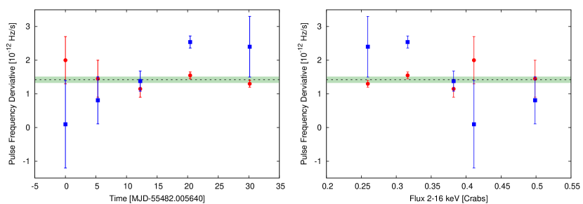
Figure 1.— Left Panel: Time evolution of the pulse frequency derivative of IGR J17480–2446 for the fundamental (blue squares) and first overtone (red circles). The dotted line refers to the long-term average $\dot{\nu}$ of the fundamental reported in Cavecchi et al. (2011), with the green band being the 68% confidence interval calculated with MC simulations. Each data point is measured in a $\sim 4-9$d data interval and the errors are calculated by means of MC simulations (see Section 2). All the data points are consistent with the green confidence interval bar with the exception of the 4th data point of the fundamental which can be considered an outlier (see Section 3.1 for a discussion). Right Panel: Pulse frequency derivative vs. X-ray flux. The meaning of symbols is the same as in the left panel. No trend is visible in the data suggesting that short-term $\dot{\nu}$ measurements have a very weak or no dependence on the X-ray flux.

3. Results of Coherent Analysis

We produce two different outputs: the pulse frequency derivative as it evolves in time (Figure 1, left panel) and as a function of the X-ray flux (Figure 1, right panel). The parameter shows no clear evolution with time and the distribution of points around the long-term average $\dot{\nu}$ is consistent with random fluctuations due to measurement errors, with the exception of one outlier in the fourth data segment of the fundamental.

Under the assumption that the X-ray flux tracks the mass accretion rate $\dot{M}$ and that our five measured pulse frequency derivatives represent short-term instantaneous spin frequency derivatives, we expect to see $\dot{\nu}\propto\,f^{\gamma}_{X}$, where $\gamma=\frac{6}{7}$ in the simplest accretion model (see for example Ghosh & Lamb 1979, Bildsten et al. 1997). From the right panel of Figure 1 we see no clear dependence of $\dot{\nu}$ from $f_{X}$. All short term pulse frequency derivatives are consistent within 1 $\sigma$ with the average long-term pulse frequency derivative $\dot{\nu}=1.42(5)\times 10^{-12}$, reported by Cavecchi et al. (2011), except the second data point of the fundamental frequency which deviates by more than 3$\sigma$ and is the same outlier seen in the left panel of Figure 1 (see Section 3.1 for further discussion of the outlier).

Finally, in Figure 2 the constant pulse frequencies are plotted against time for fundamental and first overtone. We fit each harmonic with a linear function $f(t)=k+\dot{\nu}\,t$ to extract the long-term pulse frequency derivative. The results give $\dot{\nu}$ and $k$ for the two harmonics which are consistent within the $1\sigma$ statistical errors and are both consistent within 1$\sigma$ with the long-term pulse frequency derivative reported in Cavecchi et al. (2011).

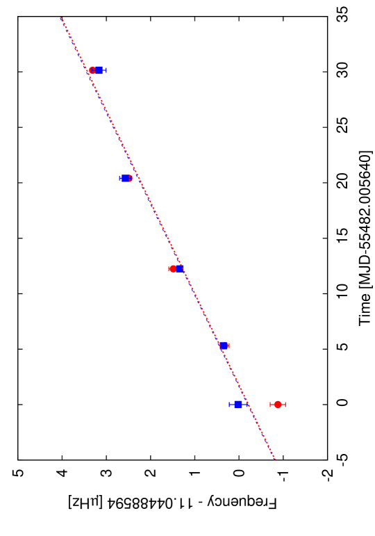
Figure 2.— Pulse frequency evolution with time. The data points refer to the same data segments used in Figure 1 and described in the text. The blue squares and red circles refer to fundamental and first overtone. Each pulse frequency is calculated with a constant pulse frequency model. Both data-sets (fundamental and first overtone) can be fit with a linear relation (blue dotted: fundamental, red dashed: first overtone) which is consistent with being the same within the statistical errors and gives a long-term $\dot{\nu}$ consistent with the value reported in Cavecchi et al. (2011).

3.1. The Spin-up of IGR J17480–2446

The results presented above strongly suggest that the long-term pulse frequency derivative reported by Cavecchi et al. (2011) is indeed the long term spin frequency derivative of IGR J17480–2446 . There are however two points that need further discussion before drawing a firm conclusion from our data analysis: the meaning of the outlier in the short-term pulse frequency derivatives and the lack of correlation between $\dot{\nu}$ and $f_{X}$.

Although the outlier indicates a significantly larger pulse frequency derivative than the long-term average, the first overtone gives in the same data segment a $\dot{\nu}$ incompatible with the outlier and compatible with the long-term average $\dot{\nu}$. The interpretation we give to this is that the outlier does not represent a true increase in the spin frequency derivative of the NS. This can be still ascribed to timing noise, even if we are carefully calculating the statistical errors with MC simulations. MC simulations verify whether a measured $\dot{\nu}$ is significant with respect to the red noise component in the TOA residuals. This is achieved by testing whether random fluctuations in the residuals are able to produce fake $\dot{\nu}$ as strong as the measured one. Since we are looking at short time series ($\sim 4-9$days), the red noise is not stationary, as evident from Figure 3, where the data segment to which the outlier belongs is shaded. In that data segment, the highest red noise frequencies observable are comparable with the length of the data segment and the data show a simple parabolic trend which is absorbed by $\dot{\nu}$ during the fitting procedure. If this is the case, MC simulations cannot discriminate between a true spin frequency derivative and the effect of timing noise. Therefore the error bars thus calculated do not differ much from those one obtains when the errors are dominated by uncorrelated Gaussian noise (i.e., white noise). The final values of the MC errors are not, is such case, a good representation of the true statistical uncertainties. This is a limitation of the MC method. However, a similar behavior is not observed in the same data segment for the first overtone and so we ascribe this behavior to timing noise.

It is of course possible that timing noise is the result of true changes of the spin frequency and/or spin frequency derivative of the NS. Fluctuating torques have been proposed in the past as a mechanism to explain fluctuations in the NS rotation (Lamb et al., 1978). However, in this case we would expect to see identical variations of the spin parameters in both harmonics which is not observed for the outlier in IGR J17480–2446 . Furthermore it has been shown that the timing noise observed in at least two accreting millisecond pulsars (Watts et al., 2008; Patruno et al., 2010) cannot be ascribed to true variations of the neutron star spin parameters since these require unphysical large torque variations.

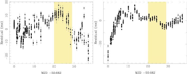
Figure 3.— Timing residuals for the fundamental (left panel) and first overtone (right panel). The strength of timing noise for the two harmonics is comparable with an rms of the residuals for fundamental and first overtone of 5.1 and 4.9 ms respectively. The fundamental shows a stronger timing noise than the first overtone on short timescales ($\sim 1$d) for the first 15 days and the last 3 days, whereas the first overtone has a stronger noise component on longer timescales. The yellow shaded area refer to the data segment where the fundamental pulse frequency derivative shows an outlier (see text for a discussion)

The fact that $\dot{\nu}$ is not proportional to $f_{X}$ can be a consequence of different phenomena. The X-ray flux might be not a good tracer of $\dot{M}$ as has been already seen in several other X-ray binaries (van der Klis, 2001). Our data suggest that $\dot{\nu}\approx\rm\,const$ over an X-ray flux variation of a factor $\approx\,2$. An approximately constant bolometric flux might therefore easily explain the observations.

Another possibility is that $\dot{\nu}\propto\,f_{X}^{6/7}$ is valid only if the accretion disk is a standard thin disk under the rather unrealistic assumption that radiation pressure is not important in determining the inner disk structure (Psaltis & Chakrabarty, 1999). Andersson et al. (2005) suggest that this assumption is not correct already at accretion rates of a few percent Eddington. Since IGR J17480–2446 is accreting at least at $\dot{M}>5\%$ Eddington with peaks exceeding 37%, it is not unreasonable to assume that radiation pressure plays a role in determining the inner disk structure. The disk-magnetosphere interaction region is also more complex than usually assumed (see e.g., Rappaport et al. 2004, D’Angelo & Spruit 2010, Kajava et al. 2011, Patruno et al. 2012), and $\dot{\nu}$ might have a weaker dependence on the bolometric flux than usually assumed.

We conclude therefore that the interpretation of the long term $\dot{\nu}$ as being the spin frequency derivative of IGR J17480–2446 is supported by the observations, with the outlier most likely explained by unmodeled timing noise and the lack of correlation between the short term $\dot{\nu}$ and $f_{X}$, which is not surprising, since the expectation of such correlations is based on assumptions about the accretion process which may not be valid.

4. Evolutionary History of IGR J17480–2446

The present RLOF spin-up epoch has been preceded by two earlier epochs in which the binary was still detached. In the first dipole spin-down epoch, the newly born NS has an initial rotation rate $\Omega_{0}$ (spin $\nu_{0}=\Omega_{0}/2\pi$) and dipole moment $\mu_{0}$. The magneto dipole torque dominates this epoch until the wind of the companion penetrates the light cylinder and the NS is spun down by wind torques. When this second epoch starts, the NS has rotational rate and dipole moments $\Omega_{1}$ and $\mu_{1}$ respectively. In this section we present an evolutionary history of these three epochs to determine the evolution of the NS spin in IGR J17480–2446 . The dipole moment decay induced by the spin-down of the NS in the superfluid-superconducting core of the star is assumed to be an essential factor during the spin-down epochs. We summarize the duration and the symbols used for each evolutionary phase in Table 3.

Table 3Evolutionary History of IGR J17480–2446

Epoch	Duration (yr)	$\mu_{i}$	$\mu_{f}$	$\Omega_{i}$	$\Omega_{f}$
Dipole spin-down	$10^{7}$	$\mu_{0}$	$\mu_{1}=\mu_{0}$	$\Omega_{0}$	$\Omega_{1}$
Wind spin-down	$10^{7}-10^{8}$	$\mu_{1}=\mu_{0}$	$\mu_{2}$	$\Omega_{1}$	$\Omega_{2}$
RLOF spin-up	$10^{7}-10^{8}$	$\mu_{2}$	$\mu_{2}$	$\Omega_{2}$	$\Omega_{3}$

4.1. Duration of the Roche Lobe Overflow Epoch

In the present RLOF spin-up epoch, the 2-16 keV X-ray luminosity of IGR J17480–2446 spans values between $9\times 10^{36}\rm\,erg\,s^{-1}$ and $6.5\times 10^{37}\rm\,erg\,s^{-1}$ for an assumed distance of 5.5 kpc (Ortolani et al., 2007). This luminosity has to be considered a lower limit given that the bolometric luminosity is expected to be higher than the X-ray luminosity. Linares et al. (2012) estimated a bolometric luminosity at the peak of the outburst of about $50\%$ the Eddington limit for $d=6.3$ kpc ($L_{Edd}=2.5\times 10^{38}\rm\,erg\,s^{-1}$). The maximum mass accretion rate is therefore

$$\dot{M}=\frac{LR_{NS}}{GM_{NS}}\simeq 5\times 10^{17}\left(\frac{d}{5.5{\rm\,kpc}}\right)^{2}\frac{R_{6}}{M_{1.4}}\rm\,g\,s^{-1},$$

where $G$ is the gravitational constant, $M_{NS}$ and $R_{NS}$ are the mass and radius of the NS, and $M_{1.4}$ and $R_{6}$ are the mass of the NS in units of $1.4\,M_{\odot}$ and the radius in units of $10^{6}\rm\,cm$ respectively. The average mass accretion rate during the outburst has a value approximately half the peak value, and we assume it is $\langle\,\dot{M}\,\rangle\,=2\times 10^{17}\rm\,g\,s^{-1}$, in agreement with the value reported by Degenaar & Wijnands (2011).

The inner radius $r_{A}$ of the accretion disk is determined by the balance between the magnetic stresses in the NS magnetosphere and the material stresses of the accretion disk (Ghosh & Lamb, 1979):

$$r_{A}=\left(\frac{{\mu}^{2}}{\dot{M}}\right)^{2/7}\left(GM_{NS}\right)^{-1/7}.$$ (1)

where $\mu$ is the dipole magnetic moment of the star. The Keplerian rotation rate at the inner radius of the disk

$$\Omega_{K}(r_{A})=\left(\frac{GM_{NS}}{{r_{A}}^{3}}\right)^{1/2}=\left(\frac{{\mu}^{2}}{\dot{M}}\right)^{-3/7}\left(GM_{NS}\right)^{5/7}$$ (2)

determines the torques on the NS applied by the accretion flow and the induced distortions of the magnetic field. These torques operate as long as $\Omega_{\*}$ is not equal to $\Omega_{K}(r_{A})$, so that the star spins up or down toward an equilibrium rotation rate $\Omega_{eq}=\Omega_{K}(r_{A})$. If any of the QPO frequencies (see Altamirano et al. 2010) is interpreted as the eventual spin equilibrium frequency of the NS, the present rotation rate will give an estimate of the dipole moment of the NS. This identification however, is not straightforward. QPO frequencies reflect modes of oscillation in the accretion flow that are excited in the interacting disk-NS system to some amplitude to effect the luminosity signal. A particular QPO frequency band might be defined by some oscillation mode of the disk or by a beat or resonance between the NS and a disk mode. Disk modes are fundamentally effected by rotation and imprinted by the frequency scale of the disk rotation, Keplerian in most parts of the disk, but necessarily and significantly deviating from the Keplerian rate at the inner boundary where the effect of the NS magnetosphere is important. This results in frequencies of epicyclic (radial) disk oscillations to be somewhat higher than the non-Keplerian rotation frequency at the inner disk boundary or transition region (Alpar & Psaltis, 2008). The presence of a sequence of QPO frequencies may be due to the presence of several multipole components of the neutron star magnetic field, so that the boundary between the disk and the NS magnetosphere is convoluted with a sequence of decreasing “stopping radii”, smaller than the conventional Alfven radius given in Equation (1) and increasing Kepler frequencies corresponding to higher multipoles of the NS magnetic field (Alpar 2011). We assume that one of the observed range of QPO frequencies $\nu_{i}$ is close to the Keplerian rotation rate $\Omega_{K}(r_{A})$ near the Alfvén radius,

$$\nu_{i}\cong\frac{\Omega_{K}(r_{A})}{2\pi}$$

yielding the estimates

$$\mu \cong (2\pi\nu_{i})^{-7/6}\dot{M}^{1/2}(GM_{NS})^{5/6}$$ (3)

$$\mu = 1.3\times 10^{26}\rm\,G\;{cm}^{3}\left(\frac{\nu_{i}}{kHz}\right)^{-7/6}\langle\dot{M}\rangle^{1/2}M_{1.4}^{5/6}$$

for the dipole moment. In these estimates we use $\langle\dot{M}\rangle$ to mean the mass accretion rate averaged over the outburst length and it is normalized to $2\times 10^{17}\rm\,g\,\;s^{-1}$;

Table 4QPO Frequency Model for IGR J17480–2446

QPO Frequency $\nu_{i}$	$\mu$	$B$ Field	$\dot{\nu}$	$t_{su,QPO}$
$(\rm\,Hz)$	$(10^{27}\rm\,G\,cm^{3})$	($10^{9}$G)	$(10^{-12})$	$(10^{7}\rm\,yr)$
48	5	10	1.6	1.8
173	1	2	1.1	2.8
814	0.2	0.4	0.6	4.6

The values of the magnetic dipole moment are reported in Table 4. If we take the NS to be already in equilibrium at the present spin frequency of 11 Hz, then $\mu\cong 2\times 10^{28}\rm\,G\,{cm}^{3}$ and a $B$ field at the poles of $4\times 10^{10}$G where we have used:

$$\mu_{30}=0.6f^{7/6}\left(\frac{d}{5.5{\rm\,kpc}}\right){R_{6}}^{1/2}M_{1.4}^{1/3}\nu^{-7/6}$$ (4)

Here $f$ takes account of the possibility that the observed frequency is not the Kepler frequency but some related frequency at the disk boundary: e.g., $f\sim 1.5-2$ for the epicyclic frequency (e.g., Alpar & Psaltis 2008). This uncertainty makes the field estimates somewhat higher.
The torque applied by the accretion disk on the NS is usually assumed to be:

$$N=\dot{M}(GM_{NS}r_{A})^{1/2}F(\omega)$$ (5)

with the dimensionless torque $F(\omega)$ describing the dependence on the fastness parameter $\omega\equiv\Omega_{\*}/\Omega_{K}(r_{A})$, is likely of the form

$$F(\omega)=1-\omega^{p}$$

with the exponent $p\sim 2$ (Ertan et al., 2009). If IGR J17480–2446 is as yet at the beginning of its spin-up epoch, then $\omega<<1$, $F(\omega)\cong 1$, giving constant $\dot{\nu}$ and expected spin frequency derivatives

$$\dot{\nu}\cong 6\times 10^{-13}{\rm\,Hz\;s^{-1}}\frac{\langle\dot{M}\rangle M_{1.4}^{2/3}}{I_{45}\left(\frac{\nu_{i}}{\rm\,kHz}\right)^{1/3}}$$ (6)

where $I_{45}$ is the NS moment of inertia in units of $10^{45}\rm\,g\,cm^{2}$. These estimates of $\dot{\nu}$ are also given in Table 4. With any of the QPO $\nu_{i}$ this gives $\dot{\nu}\sim 10^{-12}\rm\,Hz\;s^{-1}$. If the system is already in equilibrium $\dot{\nu}$ would be fluctuating in sign with rms values much smaller than $10^{-12}\rm\,Hz\;s^{-1}$, which is however not observed (see Section 3 and Figures 1 and  2).

The spin-up age up to the present is then

$$t_{su,QPO}\cong 5\times 10^{5}\;yr\frac{I_{45}{\left(\frac{\nu_{i}}{kHz}\right)}^{1/3}}{\langle\dot{M}\rangle M_{1.4}^{2/3}\Delta}.$$ (7)

where $\Delta$ is the (unknown) duty cycle of the binary. If we assume $\Delta\sim 0.01$, the maximum estimated time in the spin-up epoch up to now is $\approx 5\times 10^{7}$ yr corresponding to $\nu_{i}=814\rm\,Hz$ (see Table 4). If any of the QPO frequencies is interpreted as the eventual equilibrium frequency, then the time spent in the current spin-up epoch is a small fraction of the age of the system. Even if the system were already in equilibrium at $\nu=11\rm\,Hz$ then it must have reached equilibrium in the short time

$$t_{su}\cong\frac{\nu}{\dot{\nu}\,\Delta}\simeq 2.5\times 10^{7}yr.$$ (8)

4.2. Duration of the Dipole Spin-down Epoch

New born NSs have a distribution of rotation rates $\Omega_{0}\sim 1-300$ rad s^-1 and dipole magnetic moments $\mu_{0}\sim 10^{29}-10^{30}$ G cm³ (Faucher-Giguère & Kaspi, 2006). The NS is active as a pulsar until the magnetospheric voltage falls below a critical threshold (the “pulsar death line”). For conventional radio pulsars the epoch of pulsar activity lasts for 10⁶-10⁷ yr. No evidence of magnetic field decay is seen in the pulsar population during this active epoch. The lower limit for an exponential decay time is 10⁷ yr.

If the magnetic dipole moment decayed in proportion to the rotation rate, due to flux-line vortex line coupling (Srinivasan et al., 1990),

$$\mu(t)=\mu_{0}\frac{\Omega(t)}{\Omega_{0}}.$$ (9)

the spin-down would follow a power law with braking index $\cong 5$. More detailed considerations of flux-line motion indicates that the simple scaling in Equation (12) is a likely to be a good description for the evolution (Jahan-Miri, 2000).

The vortex-flux coupling leads to the decay of magnetic flux in the NS superfluid neutron-superconducting proton core. For the total dipole moment to decay, the flux expelled from the core must diffuse through the highly conducting crust. The decay time through the crust is estimated to be 10⁷ yr. This is supported by the limits on exponential decay of the dipole moment from population analysis of the radio pulsars. Ongoing dipole spin-down on time scales much longer than 10⁷ yr, that is, beyond the typical duration of the epoch of radio pulsar emission, will be effected by the power law decay of the dipole moment due to flux-vortex coupling.

Whether pulsar activity has ceased or not, vacuum dipole spin-down will continue until the wind captured from the companion penetrates the light cylinder. The captured wind loses angular momentum in a shock and will accrete towards the NS down to a stopping radius $\sim r_{A}$. The wind will be able to affect the torque on the neutron star when

$$r_{A}(\mu_{0},\dot{M}_{wNS}){\thinspace\hbox to0.0pt{\raise 2.15277pt\hbox{$\scriptstyle{<}$}\hss}{\lower 1.29167pt\hbox{$\scriptstyle{\sim}$}}\thinspace}r_{LC}\equiv\frac{c}{\Omega_{1}}.$$ (10)

with $\dot{M}_{wNS}$ denoting the wind captured by the NS. After this point, spin-down will proceed under the effect of the inflowing wind. From Equation (10) the rotation rate $\Omega_{1}$ at the beginning of the wind spin-down epoch is

$$\Omega_{1}\cong 24{\rm\,rad\;s^{-1}}\mu_{1,29}^{-4/7}\dot{M}_{wNS,13}^{2/7}M_{1.4}^{1/7}$$ (11)

where $\dot{M}_{wNS,13}$ is the mass inflow rate arriving at $r_{A}$ in units of $10^{13}$ g  s^-1. If we first assume that flux-vortex coupling has no effect, the dipole spin-down proceeds with a constant dipole moment and braking index 3:

$$\dot{\Omega}=-K\Omega^{3}=-\frac{4\mu^{2}\pi}{3c^{3}I}\Omega^{3}$$ (12)

where $c$ is the speed of light and $I$ is the NS moment of inertia. The duration of the dipole spin-down epoch, until the rotation rate $\Omega_{1}$ is reached is given by

$$t_{n=3} \equiv \frac{P_{1}}{2\dot{P}}=-\frac{\Omega_{1}}{2\dot{\Omega}}$$ (13)

$$\cong 10^{10}yr\;\mu_{1,29}^{-2}\Omega_{1}^{-2}$$

$$\cong 2.5\times 10^{6}yr\;\mu_{0,30}^{-6/7}\dot{M}_{wNS,13}^{-4/7}M_{1.4}^{-2/7}$$

where we have used Equations (11) and (12) and $I=10^{45}\rm\,g\,cm^{2}$. In the last line of Equation (13) we have assumed that the magnetic field does not decay during the dipole spin-down epoch, so that the dipole moment $\mu_{1}$ at the end of this epoch is still the dipole moment $\mu_{0}$ of the NS at birth. Since the lifetime thus obtained is not much smaller than the crust diffusion timescale of 10⁷ yr, it might be necessary to take the vortex-flux coupling and the induced decay of the dipole magnetic moment into account. The correct estimate of dipole spin-down epoch, incorporating flux decay according to Equation (9) proceeds with braking index 5. We obtain

$$t_{n=5} \equiv \frac{P_{1}}{4\dot{P}}=-\frac{\Omega_{1}}{4\dot{\Omega}}$$

$$\cong 5\times 10^{9}yr\;\mu_{1,29}^{-2}\Omega_{1}^{-4}$$

$$\cong 1.5\times 10^{4}yr\;\mu_{1,29}^{2/7}\dot{M}_{wNS,13}^{-8/7}M_{1.4}^{-4/7}.$$

Relating the magnetic moment $\mu_{1}$ and rotation rate $\Omega_{1}$ at the end of dipole spin-down to the initial values $\mu_{0}$ and $\Omega_{0}$ with Equation (9)

$$\mu_{1,29}=10\mu_{0,30}\frac{\Omega_{1}}{\Omega_{0}},$$ (15)

and using Equation (11) we obtain

$$t_{n=5}\cong 2\times 10^{4}y\;\mu_{0,30}^{2/11}\left[\frac{\Omega_{0}}{10{\rm\,rad\,s^{-1}}}\right]^{-2/11}\dot{M}_{wNS,13}^{-12/11}M_{1.4}^{-6/11}.$$ (16)

This value is shorter than the typical field diffusion time scale through the NS crust (${\thinspace\hbox to0.0pt{\raise 2.15277pt\hbox{$\scriptstyle{>}$}\hss}{\lower 1.29167pt\hbox{$\scriptstyle{\sim}$}}\thinspace}10^{7}$yr) and therefore Equation (16) cannot be used self-consistently for $\mu_{0}\sim 10^{29}-10^{30}\rm\,G\,cm^{3}$. If one ignores the field decay and assumes a typical $\mu_{0}=10^{29-30}\rm\,G\,cm^{3}$ in Equation (13) then the dipole spin down age is $\sim 10^{7}$ yr.

4.3. Duration of the Wind Accretion Spin-down Epoch

Wind accretion (Edgar 2004, Theuns & Jorissen 1993; Theuns et al. 1996, Pfahl et al. 2002) proceeds by Bondi-Hoyle like capture of material from the companion’s wind, which is then channeled toward the NS by outward transport of angular momentum in traversing a shock front. The wind mass loss rate from a $\sim 1\,M_{\odot}$ main sequence companion is $\dot{M}_{wind}\sim 10^{12}\rm\,g\,s^{-1}$, which is low when compared to the present day mass accretion rate, driven by RLOF. Even considering a sub-giant phase of a $\sim 1\,M_{\odot}$ donor star, the wind loss rate will increase only slightly, reaching $\dot{M}_{wind}\sim 10^{13}\rm\,g\,s^{-1}$ for sub-giant stars (see for example Reimers 1975, 1978). Only a fraction of this wind will be captured to flow towards the NS, with $\dot{M}/\dot{M}_{wind}$ as low as $\sim 10^{-2}$ (Nagae et al., 2004). However, since the orbit of IGR J17480–2446 shows stringent upper limits on the eccentricity ($e<10^{-3}$, Papitto et al. 2011) tidal circularization has probably already taken place and it is likely that the donor star is rotating synchronously with the orbit, since the circularization timescale is typically larger than the synchronization timescale (see for example Hurley et al. 2002). The large rotation of the donor ($v_{rot}\simeq 70\rm\,km\,s^{-1}$) can boost the wind loss rate by a large factor of the order of $10^{2-3}$ when compared with typical isolated stars of similar mass at the same evolutionary stage. The captured wind might be therefore comparably higher, with values of $\dot{M}_{wNS}\sim 10^{13-14}\rm\,g\,s^{-1}$.

The NS is spinning rapidly within this wind of low specific angular momentum. For our purposes of estimating the duration of the spin-down epoch it will be enough to take a constant torque, giving the spin-down rate:

$$\dot{\Omega} = -\frac{\dot{M}_{wNS}}{I}\left(GM_{NS}r_{A}\right)^{1/2}$$ (17)

$$= -\left(\dot{M}_{wNS}\right)^{6/7}\frac{\mu^{2/7}}{I}\left(GM_{NS}\right)^{3/7}$$

$$= -4.9\times 10^{-15}{\rm\,rad\,s^{-1}}\dot{M}_{wNS,13}^{6/7}\mu_{1,29}^{2/7}M_{1.4}^{3/7}I_{45}^{-1}$$ (18)

Using Equations (9) and (15) one can find the spin-down in wind and field decay solutions

$${\mu(t)}^{5/7} = {\mu_{1}}^{5/7}-5/7C^{\prime}t$$ (19)

$${\Omega(t)}^{5/7} = {\Omega_{1}}^{5/7}-5/7Ct$$ (20)

$$C \equiv \left(\frac{\mu_{1}}{\Omega_{1}}\right)^{2/7}\frac{{\dot{M}_{wNS}}^{6/7}(GM_{NS})^{3/7}}{I}$$

$$C^{\prime} \equiv \frac{\mu_{1}}{\Omega_{1}}\frac{{\dot{M}_{wNS}}^{6/7}(GM_{NS})^{3/7}}{I}.$$

Since the magnetic moment does not change after the wind spin-down epoch, $\mu_{2}$ at the end of the wind spin-down epoch is just the magnetic moment in the present RLOF spin-up epoch as estimated above. By assuming that $\Omega(t_{sd})=\Omega_{2}<<\Omega_{1}$ and $\mu_{2}<<\mu_{1}$, we obtain

$$t_{sd} = \frac{7}{5}\frac{\Omega_{1}}{{\mu_{1}}^{2/7}}\frac{I}{{\dot{M}_{wNS}}^{6/7}(GM_{NS})^{3/7}}$$

$$\cong 3\times 10^{7}\;yr\;I_{45}\;\mu_{0,30}^{-6/7}\dot{M}_{wNS,13}^{-4/7}M_{1.4}^{-2/7}.$$

where we have assumed that $\mu_{1}=\mu_{0}$ as found at the end of the previous section.

From the calculations presented in Equation (4.3) we see that for a captured wind of $\dot{M}_{wind,NS}\sim\,10^{-2}\cdot\,\dot{M}_{wind}\sim 10^{13}-10^{14}\rm\,g\,s^{-1}$, the spin-down epoch lasts for a time $10^{7-8}$yr, much shorter than the age of the cluster ($\sim 10^{10}$yr) for an assumed $\mu_{1}=\mu_{0}=10^{29-30}\rm\,G\,cm^{3}$. If more wind is accreted, as described for example in the focused accretion model of Podsiadlowski & Mohamed (2007) , the wind spin-down epoch would be further shortened if the wind still carries low angular momentum. If the wind has instead large angular momentum because it is focused through the Lagrangian point $L_{1}$, the RLOF epoch would be further shortened.

4.4. Incompatibility with a Spin Equilibrium Scenario

In the previous section we have seen that IGR J17480–2446 is not close to equilibrium since it exhibits a strong spin-up during the outburst. Several other considerations on the evolutionary history of IGR J17480–2446 also suggest that the NS is currently spinning up. According to the spin evolution history, the present 11 Hz spin frequency does not represent a special frequency. It remains to be explained whether the conclusion that the binary has currently completed only the first few million years since the onset of the RLOF, a phase which lasts for $\sim 10^{9}$ yr, requires any special pleading.

If we assume that the observed spin-up and outburst duration represent the typical values of an outburst of IGR J17480–2446 , then the pulsar spins up by $\dot{\nu}\;\Delta\,t_{o}\simeq 7\times 10^{-6}\rm\,Hz$ at each outburst, where $\Delta\,t_{o}$ is the outburst length (55 days). If the NS is dominated by magneto dipole spin-down during quiescence, as proposed for some accreting millisecond pulsars (Hartman et al. 2008; Hartman et al. 2009; Hartman et al. 2011, Patruno et al. 2010, Papitto et al. 2011, Riggio et al. 2011) then a balance of the spin-up requires a magnetic field $B\simeq 10^{11}\rm\,G$ and a recurrence time of $\sim 15$ yr to provide a spin-down with the necessary magnitude calculated via the expression (Spitkovsky, 2006):

$$\dot{\nu}_{sd}=-\frac{\mu^{2}\left(\frac{2\pi\nu}{c}\right)^{3}\left(1+{\rm\,sin}^{2}\alpha\right)}{2\pi\,I}$$ (22)

where $\alpha$ is the offset angle between the rotational and magnetic field axes. The spin down would then be of the order of $-10^{-14}\rm\,Hz\,s^{-1}$.

However, as discussed in Section 1, different estimates of the $B$ field of IGR J17480–2446 suggest $B\sim 10^{9}-10^{10}$G. Such a $B$ value requires a recurrence time of $\sim 10^{2}-10^{3}$ yr which is not compatible with a binary evolution scenario with the donor in an RLOF phase. The mass transfer rate (equal to the outburst mass accretion rate averaged over the source duty cycle) would then average to $\dot{M}\sim 10^{13}-10^{14}\rm\,g\,s^{-1}$, a value too small for an evolved donor or even a main sequence star with $M>0.8\,M_{\odot}$ (typical values being $\sim 10^{15}-10^{16}\rm\,g\,s^{-1}$).

5. Constraints on the Donor Mass and Binary Parameters

The mass function of IGR J17480–2446 has been reported in Papitto et al. (2011) and corresponds to a minimum donor mass of 0.4$M_{\odot}$ for a neutron star of $1.4\,M_{\odot}$. The location of IGR J17480–2446 in the globular cluster Terzan 5 allows to place further constraints on the donor mass. Terzan 5 is composed by two populations of stars: one with sub-solar metallicity ($Z=0.01$, $Y=0.26$) and one with supra-solar metallicity ($Z=0.03$, $Y=0.29$; see Ferraro et al. 2009). One interpretation of these discrepant metallicities and Helium abundances is that the cluster is composed by two different populations of stars with ages of $12\pm 1$ Gyr (metal poor) and $6\pm 2$ Gyr (metal rich). If we assume that the donor star belongs to the first population, strong constraints can be placed on the donor star. Since the orbital period of IGR J17480–2446 is $\approx 21$ hr, and assuming a minimum NS mass of 1.2$\,M_{\odot}$, the minimum orbital separation of the system is $A\approx 0.02$ AU. By using the Roche lobe approximation of Eggleton (1983):

$$R_{L}=\frac{0.49\,A\,q^{2/3}}{0.6q^{2/3}+\rm\,ln\left(1+q^{1/3}\right)}$$ (23)

with $q=M_{d}/M_{NS}$ being the ratio of the donor and accretor mass, the minimum possible Roche lobe radius that corresponds to the minimum orbital separation and the minimum mass ratio ($M_{d}=0.4\,M_{\odot}$, $M_{NS}=1.2\,M_{\odot}$) is 1.1$R_{\odot}$. After 12 Gyr all stars with a mass $M{\thinspace\hbox to0.0pt{\raise 2.15277pt\hbox{$\scriptstyle{>}$}\hss}{\lower 1.29167pt\hbox{$\scriptstyle{\sim}$}}\thinspace}1\,M_{\odot}$ have evolved to the red giant phase and might have already turned into white dwarfs whereas all stars with $M{\thinspace\hbox to0.0pt{\raise 2.15277pt\hbox{$\scriptstyle{<}$}\hss}{\lower 1.29167pt\hbox{$\scriptstyle{\sim}$}}\thinspace}0.9\,M_{\odot}$ (i.e., the turn off mass of the metal-poor population of Terzan 5, Ferraro et al. 2009) are still on the main sequence. Considering the other extreme case of $M_{d}=1.0\,M_{\odot}$ and $M_{NS}=2.0\,M_{\odot}$, the maximum Roche lobe radius will be 1.8$R_{\odot}$.

To fill the Roche lobe therefore any possible donor star of IGR J17480–2446 has to be an evolved star that has left the main sequence and has increased its radius to fit its Roche lobe. The donor star mass falls in the range $0.9{\thinspace\hbox to0.0pt{\raise 2.15277pt\hbox{$\scriptstyle{<}$}\hss}{\lower 1.29167pt\hbox{$\scriptstyle{\sim}$}}\thinspace}\,M{\thinspace\hbox to0.0pt{\raise 2.15277pt\hbox{$\scriptstyle{<}$}\hss}{\lower 1.29167pt\hbox{$\scriptstyle{\sim}$}}\thinspace}\,1\,\,M_{\odot}$ and is likely to be a sub-giant. This result strongly constrains the orbital separation of the system to be in the range $0.023$-$0.026$ AU for a total mass of the binary between 2.1 ($1.2\,M_{\odot}$ NS and 0.9$\,M_{\odot}$ donor) and 3$\,M_{\odot}$ ($2\,M_{\odot}$ NS and $1\,M_{\odot}$ donor). The inclination $i$ of the binary is then constrained by using the projected semi-major axis of IGR J17480–2446 (see Table 1):

$$i={\rm\,sin^{-1}}\left(\frac{5\times 10^{-3}\rm\,AU}{A}\frac{M_{NS}+M_{d}}{M_{d}}\right)\simeq\,30^{\circ}.$$ (24)

Identical considerations apply if the donor star belongs to the metal rich population, with the difference that the turn off mass will be higher by a few tenths of solar mass and the inclination smaller by a few degrees.

All these considerations assume that irradiation of the donor star is unimportant in determining its radius. This is a good assumption given that non-negligible irradiation sets in with the onset of RLOF and we have seen that this phase has lasted for ${\thinspace\hbox to0.0pt{\raise 2.15277pt\hbox{$\scriptstyle{<}$}\hss}{\lower 1.29167pt\hbox{$\scriptstyle{\sim}$}}\thinspace}10^{7}-10^{8}$ yr. Therefore any possible donor star has filled the Roche lobe following a standard evolutionary path that does not involve irradiation of the outer envelope. The effect of irradiation might instead be important during the RLOF phase when the outermost layers of the envelope expand after absorbing the energy deposited by the X-ray radiation. The star being constrained to fit the Roche lobe will increase its mass loss through the inner Lagrangian point and boost the mass transfer rate. The average X-ray power absorbed by the companion during an outburst is

$$L_{abs}=\langle\,L_{x}\rangle\left(\frac{\,R}{2\,A}\right)^{2}$$ (25)

with $\langle\,L_{x}\rangle\sim 4\times 10^{37}\rm\,erg\,s^{-1}$ being the average X-ray luminosity during an outburst. Given a duty cycle of $\Delta{\thinspace\hbox to0.0pt{\raise 2.15277pt\hbox{$\scriptstyle{<}$}\hss}{\lower 1.29167pt\hbox{$\scriptstyle{\sim}$}}\thinspace}0.005$, the long term average power absorbed by the donor will be ${\thinspace\hbox to0.0pt{\raise 2.15277pt\hbox{$\scriptstyle{<}$}\hss}{\lower 1.29167pt\hbox{$\scriptstyle{\sim}$}}\thinspace}\,10^{33}-10^{34}\rm\,erg\,s^{-1}$. This value corresponds to ${\thinspace\hbox to0.0pt{\raise 2.15277pt\hbox{$\scriptstyle{<}$}\hss}{\lower 1.29167pt\hbox{$\scriptstyle{\sim}$}}\thinspace}10\%-100\%$ of the outgoing power produced by a low mass stars in the sub-giant branch and cannot be considered negligible. The quantitative effect of irradiation can be calculated with stellar evolutionary codes and is beyond the scope of this work.

6. Discussion

We have investigated the evolutionary history of IGR J17480–2446 discussing three distinct evolutionary epochs: a dipole dominated spin-down epoch, a wind epoch and the currently observed RLOF phase. By taking into account the effect of timing noise in the X-ray pulsations we are able to confirm the long-term average spin-up of $1.4\times 10^{-12}\rm\,Hz\,s^{-1}$ observed during the 2010 outburst (Papitto et al. 2011; Cavecchi et al. 2011). If the X-ray flux represents most of the bolometric flux, the short term spin frequency derivatives $\dot{\nu}$ do not scale with the X-ray flux in the expected way. The long-term $\dot{\nu}$, however, leads to exclude a scenario in which IGR J17480–2446 has already reached spin equilibrium. A long-term spin equilibrium with magnetic dipole spin down in quiescence balancing the accretion torques in outburst is also excluded based on binary evolution considerations. The spin-up timescale suggests that IGR J17480–2446 has been spun-up in the RLOF phase for a few $10^{7}$ yr. An interpretation of the observed QPOs as the equilibrium frequencies of IGR J17480–2446 indicates a similar timescale for the spin-up epoch up to the present.

The spin-down epochs suggest that the NS in IGR J17480–2446 had reached a spin frequency of the order of $\sim 1$Hz at the onset of the RLOF phase, if we assume that the newborn NSs had typical initial values for $\Omega_{0}$ and $\mu_{0}$. This reinforces the idea that the time elapsed in RLOF has been very short, since the time required to spin-up a 1 Hz NS to 11 Hz with a spin frequency derivative of $10^{-12}\rm\,Hz\,s^{-1}$ and a duty cycle of 0.01 is a few $10^{7}$yr.

Based on these findings we conclude that IGR J17480–2446 is in an exceptionally early RLOF phase. The total spin-up timescale to transform IGR J17480–2446 from a slow pulsar ($\sim\,1\rm\,Hz$) into a millisecond one ($\nu>100\rm\,Hz$) is ${\thinspace\hbox to0.0pt{\raise 2.15277pt\hbox{$\scriptstyle{>}$}\hss}{\lower 1.29167pt\hbox{$\scriptstyle{\sim}$}}\thinspace}10^{8}-10^{9}$yr. Since the current RLOF phase will last for $\sim 10^{9}$yr, we would expect to observe today $\sim 1-10$ accreting millisecond pulsars that have followed a similar evolutionary history as IGR J17480–2446 . The accreting millisecond pulsar SAX J1748.9-2021 ($\nu\simeq 442\rm\,Hz$) in the globular cluster NGC 6440 has a companion with mass and orbital period compatible with being in a slightly evolved post main sequence phase (Altamirano et al., 2008). It is likely that the companion of SAX J1748.9-2021 has followed an evolutionary history similar to IGR J17480–2446 with the difference that it spent a longer time in the RLOF phase thus turning its NS into a millisecond pulsar. The scenario outlined above is compatible with the observed population of accreting pulsars, although it is difficult to assess the problem in a robust way given the small number statistics. It is also possible that dynamical interactions have played a role by decreasing the number of similar systems in globular clusters via ionization interactions. This however requires further investigations along with detailed binary evolution calculations.

The prior spin-down history gives results which are not compatible with a binary having an age of several $10^{9}$ yr as expected if IGR J17480–2446 is primordial or if it has not suffered exchange interactions in the last few $10^{9}$ yr. Different formation scenarios are available to explain the apparent discrepancy between the age of the cluster and the binary. A first possibility is that a recent dynamical encounter has played a role in forming the binary or in accelerating the onset of the RLOF phase. If an exchange interaction has taken place in the last few $10^{7}-10^{8}$ yr then this would explain why the apparent age of IGR J17480–2446 is so short compared with the age of the cluster. The location of IGR J17480–2446 in the high mass and high central density cluster Terzan 5 suggests that the interaction rate might be particularly high in this environment. Dynamical simulations to calculate the typical interaction rates in the core of Terzan 5 are required to assess this question.

A second possibility for the origin of IGR J17480–2446 is formation of the accreting pulsar via accretion induced collapse (AIC) of a massive white dwarf (Miyaji et al. 1980, Nomoto 1987). In this scenario a ONeMg white dwarf accretes matter until its mass exceeds the Chandrasekhar limit and it collapses to form an NS via electron captures on Mg and Ne nuclei. In this case the binary must have gone through a preliminary contact phase during which the white dwarf was accreting from a donor star in RLOF. During the collapse approximately 0.2$\,M_{\odot}$ are ejected from the binary (see for example van den Heuvel 2011 for a discussion) which causes a sudden expansion of the orbit turning the system into a detached binary. At this point the binary follows the three evolutionary epochs described in Section 4 with the NS age set by the onset of AIC. The formation of NSs from AIC has been discussed by Lyne et al. (1996) to explain the young radio pulsar population in globular clusters. Lyne et al. note that the formation rate of young pulsars in globular clusters is larger than that of millisecond pulsars in globular clusters. The young pulsars are found in metal rich globular clusters with high mass and high central densities, like Terzan 5 (Lyne et al. 1996; Boyles et al. 2011). Further evidence that globular clusters might contain young NSs was also presented by Freire et al. (2011), who reported the discovery of the youngest millisecond pulsar ever found in the globular cluster NGC 6624, with a characteristic age $t<24$ Myr (see also Lyne et al. 1987 and Cognrd et al. 1996 on the “young” millisecond pulsar PSR 1821-24A in the globular cluster M28). We can therefore speculate that a similar evolutionary process has taken place for IGR J17480–2446 thus explaining the relatively short lifetime of the NS through the dipole and wind spin-down and present RLOF spin-up epochs.

A possible test for the AIC scenario can be performed by measuring the gravitational mass of the NS in IGR J17480–2446 . Since the RLOF phase has lasted for a very short time, the NS mass is currently almost identical to the value expected from the AIC scenario, which is $M\simeq 1.25\,M_{\odot}$. A gravitational NS mass larger than this value would immediately rule out the AIC scenario.

References

- Alpar (2011) Alpar M.A., 2011, MNRAS, submitted
- Alpar & Psaltis (2008) Alpar M.A., Psaltis D., Dec. 2008, MNRAS, 391, 1472
- Alpar et al. (1982) Alpar M.A., Cheng A.F., et al., Dec. 1982, Nature, 300, 728
- Altamirano et al. (2008) Altamirano D., Casella P., et al., Feb. 2008, ApJ, 674, L45
- Altamirano et al. (2010) Altamirano D., Homan J., et al., Oct. 2010, The Astronomer’s Telegram, 2952, 1
- Bordas et al. (2010) Bordas, P., Kuulkers, E., Alfonso-Garzón, J., et al. 2010, The Astronomer’s Telegram, 2919, 1
- Andersson et al. (2005) Andersson N., Glampedakis K., et al., Aug. 2005, MNRAS, 361, 1153
- Bildsten et al. (1997) Bildsten L., Chakrabarty D., et al., Dec. 1997, ApJS, 113, 367
- Boyles et al. (2011) Boyles J., Lorimer D.R., et al., Nov. 2011, ApJ, 742, 51
- Cavecchi et al. (2011) Cavecchi Y., Patruno A., et al., Oct. 2011, ApJ, 740, L8
- Chenevez et al. (2010) Chenevez J., Kuulkers E., et al., Oct. 2010, The Astronomer’s Telegram, 2924, 1
- Cognrd et al. (1996) Cognard, I., Bourgois, G., Lestrade, J.-F., et al. 1996, A&A, 311, 179
- D’Angelo & Spruit (2010) D’Angelo C.R., Spruit H.C., Aug. 2010, MNRAS, 406, 1208
- Degenaar & Wijnands (2011) Degenaar N., Wijnands R., Jun. 2011, MNRAS, 414, L50
- Edgar (2004) Edgar R., Sep. 2004, New A Rev., 48, 843
- Eggleton (1983) Eggleton P.P., May 1983, ApJ, 268, 368
- Ertan et al. (2009) Ertan Ü., Ekşi K.Y., et al., Sep. 2009, ApJ, 702, 1309
- Faucher-Giguère & Kaspi (2006) Faucher-Giguère C.A., Kaspi V.M., May 2006, ApJ, 643, 332
- Ferraro et al. (2009) Ferraro F.R., Dalessandro E., et al., Nov. 2009, Nature, 462, 483
- Freire et al. (2011) Freire P.C.C., Abdo A.A., et al., 2011, Science, 334, 1107
- Ghosh & Lamb (1979) Ghosh P., Lamb F.K., Nov. 1979, ApJ, 234, 296
- Hartman et al. (2008) Hartman J.M., Patruno A., et al., Mar. 2008, ApJ, 675, 1468
- Hartman et al. (2009) Hartman, J. M., Patruno, A., Chakrabarty, D., et al. 2009, ApJ, 702, 1673
- Hartman et al. (2011) Hartman J.M., Galloway D.K., Chakrabarty D., Jan. 2011, ApJ, 726, 26
- Haskell & Patruno (2011) Haskell B., Patruno A., Sep. 2011, ApJ, 738, L14
- Heinke et al. (2006) Heinke, C. O., Wijnands, R., Cohn, H. N., et al. 2006, ApJ, 651, 1098
- Hobbs et al. (2006) Hobbs G.B., Edwards R.T., Manchester R.N., Jun. 2006, MNRAS, 369, 655
- Hurley et al. (2002) Hurley J.R., Tout C.A., Pols O.R., Feb. 2002, MNRAS, 329, 897
- Jahan-Miri (2000) Jahan-Miri, M. 2000, ApJ, 532, 514
- Jahoda et al. (2006) Jahoda K., Markwardt C.B., et al., Apr. 2006, ApJS, 163, 401
- Kajava et al. (2011) Kajava J.J.E., Ibragimov A., et al., Oct. 2011, MNRAS, 417, 1454
- Lamb et al. (1978) Lamb F.K., Pines D., Shaham J., Oct. 1978, ApJ, 225, 582
- Linares et al. (2012) Linares, M., Altamirano, D., Chakrabarty, D., Cumming, A., & Keek, L. 2012, ApJ, 748, 82
- Linares et al. (2011b) Linares M., Chakrabarty D., van der Klis M., Jun. 2011b, ApJ, 733, L17
- Lyne et al. (1987) Lyne, A. g., Brinklow, A., Middleditch, J., Kulkarni, S. R., & Backer, D. C. 1987, Nature, 328, 399
- Lyne et al. (1996) Lyne A.G., Manchester R.N., D’Amico N., Mar. 1996, ApJ, 460, L41
- Markwardt & Strohmayer (2010) Markwardt C.B., Strohmayer T.E., Jul. 2010, ApJ, 717, L149
- Miller et al. (2011) Miller J.M., Maitra D., et al., Apr. 2011, ApJ, 731, L7
- Miyaji et al. (1980) Miyaji S., Nomoto K., et al., 1980, PASJ, 32, 303
- Nagae et al. (2004) Nagae T., Oka K., et al., May 2004, A&A, 419, 335
- Nomoto (1987) Nomoto K., Nov. 1987, ApJ, 322, 206
- Ortolani et al. (2007) Ortolani S., Barbuy B., et al., Aug. 2007, A&A, 470, 1043
- Papitto et al. (2011) Papitto A., D’Aì A., et al., Feb. 2011, A&A, 526, L3
- Patruno et al. (2010) Patruno A., Hartman J.M., et al., Jul. 2010, ApJ, 717, 1253
- Patruno et al. (2012) Patruno, A., Haskell, B., & D’Angelo, C. 2012, ApJ, 746, 9
- Pfahl et al. (2002) Pfahl E., Rappaport S., Podsiadlowski P., May 2002, ApJ, 571, L37
- Podsiadlowski & Mohamed (2007) Podsiadlowski, P., & Mohamed, S. 2007, Baltic Astronomy, 16, 26
- Pooley et al. (2010) Pooley D., Homan J., et al., Oct. 2010, The Astronomer’s Telegram, 2974, 1
- Psaltis & Chakrabarty (1999) Psaltis D., Chakrabarty D., Aug. 1999, ApJ, 521, 332
- Radhakrishnan & Srinivasan (1982) Radhakrishnan V., Srinivasan G., Dec. 1982, Current Science, 51, 1096
- Rappaport et al. (2004) Rappaport S.A., Fregeau J.M., Spruit H., May 2004, ApJ, 606, 436
- Reimers (1975) Reimers D., 1975, Memoires of the Societe Royale des Sciences de Liege, 8, 369
- Reimers (1978) Reimers D., 1978, Mitteilungen der Astronomischen Gesellschaft Hamburg, 43, 70
- Riggio et al. (2011) Riggio A., Burderi L., et al., Jul. 2011, A&A, 531, A140
- Romani (1990) Romani R.W., Oct. 1990, Nature, 347, 741
- Spitkovsky (2006) Spitkovsky A., Sep. 2006, ApJ, 648, L51
- Srinivasan et al. (1990) Srinivasan G., Bhattacharya D., et al., Jan. 1990, Current Science, 59, 31
- Strohmayer et al. (2003) Strohmayer T.E., Markwardt C.B., et al., Oct. 2003, ApJ, 596, L67
- Theuns & Jorissen (1993) Theuns T., Jorissen A., Dec. 1993, MNRAS, 265, 946
- Theuns et al. (1996) Theuns T., Boffin H.M.J., Jorissen A., Jun. 1996, MNRAS, 280, 1264
- van den Heuvel (2011) van den Heuvel E.P.J., Mar. 2011, Bulletin of the Astronomical Society of India, 39, 1
- van der Klis (2001) van der Klis M., Nov. 2001, ApJ, 561, 943
- Verbunt et al. (1990) Verbunt F., Wijers R.A.M.J., Burm H.M.G., Aug. 1990, A&A, 234, 195
- Watts et al. (2008) Watts A.L., Patruno A., van der Klis M., Nov. 2008, ApJ, 688, L37
- Wijnands & van der Klis (1998) Wijnands R., van der Klis M., Jul. 1998, Nature, 394, 344