Systematic analysis of the $B_{s}\rightarrow f_{0}\ell^{+}\ell^{-}$ in the universal extra dimension

Abstract

Using form factors enrolled to the transition matrix elements and calculated via light-cone QCD sum rules including next-to-leading order corrections in the strong coupling constant, we provide a systematic analysis of the $B_{s}\rightarrow f_{0}(980)\ell^{+}\ell^{-}$ both in the standard and universal extra dimension models. In particular, we discuss sensitivity of the differential branching ratio and various double lepton polarization asymmetries on the compactification factor of extra dimension and show how the results of the extra dimension model deviate from the standard model predictions. The order of branching ratio makes this decay mode possible to be checked at LHCb in near future.

I Introduction

It is well known that the decays of the $B_{s}$ meson are very promising tools to constrain the standard model (SM) parameters, serve to determine the elements of the Cabibbo-Kobayashi-Maskawa (CKM) matrix, enable us to understand the origin of the CP violation and help us search for new physics (NP) effects beyond the SM. One of the possible decay modes of the $B_{s}$ meson is the semileptonic $B_{s}\rightarrow f_{0}(980)\ell^{+}\ell^{-}$. This channel proceeds via flavor-changing neutral currents (FCNC) transition of $b\rightarrow s\ell^{+}\ell^{-}$ at quark level, which is induced at loop level in the SM and is therefore sensitive to NP effects. The extra dimensions as NP effects can contribute to such loop level transitions and enhance the branching ratio. It has been shown that, in the presence of a single universal extra dimension (UED) compactified on a circle with radius $R$, the branching ratios of the $B_{s}\rightarrow\eta^{(^{\prime})}\ell^{+}\ell^{-}/\nu\bar{\nu}$ and $B_{s}\rightarrow\phi\nu\bar{\nu}$ which are also based on $b\rightarrow s\ell^{+}\ell^{-}/\nu\bar{\nu}$, increase significantly at lower values of the compactification factor, $1/R$ Colangelo1 ; Colangelo2 .

In the present work, we investigate the effect of the UED on some physical observables related to the semileptonic $B_{s}\rightarrow f_{0}(980)\ell^{+}\ell^{-}$. The UED with a single extra dimension called the Appelquist, Cheng and Dobrescu (ACD) model acd , is a kind of extra dimension (ED) antoniadis1 ; antoniadis2 ; arkani which allows the SM fields (both gauge bosons and fermions) to propagate in the extra dimensions (for more details see for instance Hooper ). The ACD model has been previously applied to many decay channels. For some of them see R7624 ; wangying ; R7601 ; wangying ; fazio ; sirvanli ; kank1 ; yee ; bashiry ; aliev ; ahmet ; nihan ; cog ; Mohanta ; Haisch:2007vb and references therein.

In the SM, the effective Hamiltonian describing the $B_{s}\rightarrow f_{0}(980)\ell^{+}\ell^{-}$ transition at quark level can be written as:

$${\cal H}^{eff} = {G_{F}\alpha_{em}V_{tb}V_{ts}^{\ast}\over 2\sqrt{2}\pi}\Bigg{[}C_{9}^{eff}\bar{s}\gamma_{\mu}(1-\gamma_{5})b\,\bar{\ell}\gamma^{\mu}\ell+C_{10}\bar{s}\gamma_{\mu}(1-\gamma_{5})b\,\bar{\ell}\gamma^{\mu}\gamma_{5}\ell$$ (1)

$$- 2m_{b}C_{7}^{eff}{1\over q^{2}}\bar{s}i\sigma_{\mu\nu}q^{\nu}(1+\gamma_{5})b\,\bar{\ell}\gamma^{\mu}\ell\Bigg{]}~{}.$$

where $V_{ij}$ are elements of the CKM matrix, $\alpha_{em}$ is the fine structure constant, $G_{F}$ is the Fermi constant, and $C_{7}^{eff}$, $C_{9}^{eff}$ and $C_{10}$ are Wilson coefficients. In the ACD model, the form of the effective Hamiltonian remains unchanged but due to the interaction of the Kaluza-Klein (KK) particles with the usual SM particles and also with themselves, the Wilson coefficients are modified. This modification is done in Buras:2002ej ; R7623 ; R7626 ; R7627 ; R762777 in leading logarithmic approximation in a way that each Wilson coefficient is written in terms of some periodic functions as:

$$F(x_{t},1/R)=F_{0}(x_{t})+\sum_{n=1}^{\infty}F_{n}(x_{t},x_{n}),$$ (2)

where, $F_{0}(x_{t})$ is ordinary SM part and the other part can be written in terms of the compactification factor $1/R$, by means of the following definitions:

$$x_{t}=m_{t}^{2}/M_{W}^{2},~{}~{}~{}~{}~{}~{}~{}~{}~{}~{}~{}~{}x_{n}=m_{n}^{2}/m_{W}^{2},~{}~{}~{}~{}~{}~{}~{}~{}~{}~{}~{}~{}~{}~{}m_{n}=n/R,$$ (3)

where, $m_{t}$ is the mass of the top quark, $M_{W}$ is the mass of the $W$ boson, $m_{n}$ is the mass of the KK particles and $n=0$ corresponds to the ordinary SM particles. Few comments about the lower bound of the compactification factor are in order. From the electroweak precision tests, the lower limit for $1/R$ had been previously obtained as $250~{}GeV$ in acd ; yee if $M_{h}\geq 250~{}GeV$ expressing larger KK contributions to the low energy FCNC processes, and $300~{}GeV$ if $M_{h}\leq 250~{}GeV$. Analysis of the $B\rightarrow X_{s}\gamma$ transition and also anomalous magnetic moment had shown also that the experimental data are in a good agreement with the ACD model if $1/R\geq 300~{}GeV$ ikiuc . Taking into account the leading order (LO) contributions due to the exchange of KK modes as well as the available next-to-next-to-leading order (NNLO) corrections to also $B(B\rightarrow X_{s}\gamma)$ in the SM, the authors of Haisch:2007vb have obtained a lower bound on the inverse compactification radius $600~{}GeV$. Using the electroweak precision measurements and also some cosmological constraints, the authors of Gogoladze:2006br and Cembranos:2006gt have found that the lower limit on compactification factor is in or above the $500~{}GeV$ range. We will plot the physical observables under consideration in the range $1/R\in[200-1000]GeV$ just to clearly show how the results of the UED deviate from those of the SM and grow decreasing the $1/R$ .

The numerical values for different Wilson coefficients both in the SM and ACD model in the range $1/R\in[200-1000]GeV$ are presented in Table 1. From this Table, we see that in the ACD model, the $C_{10}$ is enhanced and $C_{7}^{eff}$ is suppressed considerably in comparison with their values in the SM.

$1/R~{}[{\rm GeV}]$	$C_{7}^{eff}$	$C_{10}$	$C_{9}^{eff}$
$200$	$-0.195212$	$-5.61658$	$4.83239+3.59874i$
$400$	$-0.266419$	$-4.65118$	$4.7538+3.54366i$
$600$	$-0.283593$	$-4.43995$	$4.7366+3.53161i$
$800$	$-0.29003$	$-4.36279$	$4.73032+3.52721i$
$1000$	$-0.293092$	$-4.32646$	$4.72736+3.52514i$
SM	$-0.298672$	$-4.26087$	$4.72202+3.52139i$

Table 1: Numerical values for $C_{7}^{eff}$, $C_{10}$ and values of $C_{9}^{eff}$ at transferred momentum square, $q^{2}=14$ for different values of $1/R$ as well as the SM

Here we should mention that, besides the aforementioned contributions, the Wilson coefficient $C_{9}^{eff}$ receives also long distance contributions from $J/\psi$ family parameterized using Breit–Wigner ansatz R8401 , i.e.,

$$Y_{\rm LD}={3\pi\over\alpha_{em}^{2}}C^{(0)}\sum_{V_{i}=\psi(1s)\cdots\psi(6s)}\ae_{i}\,{\Gamma(V_{i}\rightarrow\ell^{+}\ell^{-})m_{V_{i}}\over m_{V_{i}}^{2}-q^{2}-im_{V_{i}}\Gamma_{V_{i}}}~{},$$

where, $C^{(0)}=0.362$. As the phenomenological factors, $\ae_{i}$ have not known for the transition under consideration, we will choose the values of the $q^{2}$ which do not lie on the $J/\psi$ family resonances. This is possible in the case of the differential branching ratio and double–lepton polarization asymmetries under consideration in this work, however, to calculate the total branching ratio as well as the average double–lepton polarization asymmetries, which require integration over $q^{2}$, one should take also into account such contributions. For more details about the long distance contributions see for instance cana1 ; cana2 .

The layout of the paper is as follows. In the next section, we present the transition matrix elements expressed in terms of form factors and the formula for decay rate as well as various double lepton polarization asymmetries. In the last section, we numerically analyze the observables in terms of compactification factor, $1/R$ of the ACD model and discuss the results.

II Transition matrix elements and observables related to the $B_{s}\rightarrow f_{0}(980)\ell^{+}\ell^{-}$ channel

To find the amplitude of the decay channel in question, we need to sandwich the aforementioned effective Hamiltonian between the initial and final states. As a result, we obtain the following transition matrix elements defined in terms of form factors $F_{0}(q^{2})$, $F_{1}(q^{2})$ and $F_{T}(q^{2})$:

$$\langle f_{0}(p_{f_{0}})|\bar{s}\gamma_{\mu}\gamma_{5}b|\overline{B}_{s}(p_{B_{s}})\rangle=-i\Big{\{}F_{1}(q^{2})\Big{[}P_{\mu}-\frac{m_{B_{s}}^{2}-m_{f_{0}}^{2}}{q^{2}}q_{\mu}\Big{]}+F_{0}(q^{2})\frac{m_{B_{s}}^{2}-m_{f_{0}}^{2}}{q^{2}}q_{\mu}\Big{\}},\,\,\,$$ (4)

$$\langle{f_{0}}(p_{f_{0}})|\bar{s}\sigma_{\mu\nu}\gamma_{5}q^{\nu}b|\overline{B}_{s}(p_{B_{s}})\rangle=-\frac{F_{T}(q^{2})}{m_{B_{s}}+m_{f_{0}}}\Big{[}q^{2}P_{\mu}-(m_{B_{s}}^{2}-m_{f_{0}}^{2})q_{\mu}\Big{]},$$ (5)

where $P=p_{B_{s}}+p_{f_{0}}$ and $q=p_{B_{s}}-p_{f_{0}}$. For simplicity in some parts of calculations, it is convenient to introduce the auxiliary form factors $f_{+}$ and $f_{-}$,

$$\langle{f_{0}}(p_{f_{0}})|\bar{s}\gamma_{\mu}\gamma_{5}b|\overline{B}_{s}(p_{B_{s}})\rangle = -i\left\{f_{+}(q^{2})P_{\mu}+f_{-}(q^{2})q_{\mu}\right\}$$

such that

$$F_{1}(q^{2}) = f_{+}(q^{2})\,\,,$$

$$F_{0}(q^{2}) = f_{+}(q^{2})+\frac{q^{2}}{m_{B_{s}}^{2}-m_{f_{0}}^{2}}f_{-}(q^{2})\,\,.$$ (7)

The form factors, $F_{1}$, $F_{0}$ and $F_{T}$ are calculated via light-cone QCD sum rules both at the leading order and the next-to-leading order corrections in colangelo3 . We use the latter to analyze the considered physical observables. The fit parametrization of the form factors including next-to-leading order corrections in $\alpha_{s}$ is given as colangelo3 :

$$F_{i}(q^{2}) = \frac{F_{i}(0)}{1-a_{i}q^{2}/m_{B_{s}}^{2}+b_{i}(q^{2}/m_{B_{s}}^{2})^{2}}\,\,,$$ (8)

where $F_{i}$ denotes any function among $F_{1,0,T}$. The parameters $a_{i}$ and $b_{i}$ as well as $F_{i}(0)$ are given in Table 2.

Table 2: ${B_{s}\to f_{0}(980)}$ transition form factors including next-to-leading order corrections colangelo3 .

	$F_{i}(q^{2}=0)$	$a_{i}$	$b_{i}$
$F_{1}$	$0.238\pm 0.036$	$1.50^{+0.13}_{-0.09}$	$0.58^{+0.09}_{-0.07}$
$F_{0}$	$0.238\pm 0.036$	$0.53^{+0.14}_{-0.10}$	$-0.36^{+0.09}_{-0.08}$
$F_{T}$	$0.308\pm 0.049$	$1.46^{+0.14}_{-0.10}$	$0.58^{+0.09}_{-0.07}$

Now we proceed to calculate some observables such as differential decay rate and double lepton polarization asymmetries. With the matrix elements in terms of form factors one can easily obtain the $1/R$-dependent differential decay rate as:

$$\frac{d\Gamma(\bar{B}_{s}\to f_{0}\ell^{+}\ell^{-})}{dq^{2}}(q^{2},1/R) =\frac{G_{F}^{2}\alpha^{2}_{em}|V_{tb}|^{2}|V^{*}_{ts}|^{2}\sqrt{\lambda}}{512m_{B_{s}}^{3}\pi^{5}}\frac{v}{3q^{2}}\Bigg{[}6m_{\ell}^{2}|C_{10}(1/R)|^{2}(m_{B_{s}}^{2}-m_{f_{0}}^{2})^{2}F_{0}^{2}(q^{2})$$ (9)

$$+(q^{2}+2m_{\ell}^{2})\lambda\bigg{|}C_{9}^{eff}(q^{2},1/R)F_{1}(q^{2})+\frac{2C_{7}^{eff}(1/R)(m_{b}-m_{s})F_{T}(q^{2})}{m_{B_{s}}+m_{f_{0}}}\bigg{|}^{2}$$

$$+|C_{10}(1/R)|^{2}(q^{2}-4m_{\ell}^{2})\lambda F_{1}^{2}(q^{2})\Bigg{]},$$

with $v=\sqrt{1-\frac{4m_{\ell}^{2}}{q^{2}}}$, $\lambda=\lambda(m_{B_{s}}^{2},m_{f_{0}}^{2},q^{2})$ with $\lambda(a,b,c)=(a-b-c)^{2}-4bc$ and $m_{\ell}$ is the lepton’s mass.

To calculate the double–polarization asymmetries, we consider the polarizations of both lepton and anti-lepton, simultaneously and introduce the following spin projection operators for the lepton $\ell^{-}$ and the anti-lepton $\ell^{+}$ (see also bas1 ; bas2 ; Fukae ):

$$\Lambda_{1}~{}\!\!\! = \!\!\!~{}\frac{1}{2}(1+\gamma_{5}\!\!\not\!{s}_{i}^{-})~{},$$

$$\Lambda_{2}~{}\!\!\! = \!\!\!~{}\frac{1}{2}(1+\gamma_{5}\!\!\not\!{s}_{i}^{+})~{},$$ (10)

where $i=L,N$ and $T$ correspond to the longitudinal, normal and transversal polarizations, respectively. Now, we define the following orthogonal vectors $s^{\mu}$ in the rest frame of lepton and anti-lepton:

$$s^{-\mu}_{L}~{}\!\!\! = \!\!\!~{}\left(0,\vec{e}_{L}^{\,-}\right)=\left(0,\frac{\vec{p}_{-}}{\left|\vec{p}_{-}\right|}\right)~{},$$

$$s^{-\mu}_{N}~{}\!\!\! = \!\!\!~{}\left(0,\vec{e}_{N}^{\,-}\right)=\left(0,\frac{\vec{p}_{f_{0}}\times\vec{p}_{-}}{\left|\vec{p}_{f_{0}}\times\vec{p}_{-}\right|}\right)~{},$$

$$s^{-\mu}_{T}~{}\!\!\! = \!\!\!~{}\left(0,\vec{e}_{T}^{\,-}\right)=\left(0,\vec{e}_{N}^{\,-}\times\vec{e}_{L}^{\,-}\right)~{},$$

$$s^{+\mu}_{L}~{}\!\!\! = \!\!\!~{}\left(0,\vec{e}_{L}^{\,+}\right)=\left(0,\frac{\vec{p}_{+}}{\left|\vec{p}_{+}\right|}\right)~{},$$

$$s^{+\mu}_{N}~{}\!\!\! = \!\!\!~{}\left(0,\vec{e}_{N}^{\,+}\right)=\left(0,\frac{\vec{p}_{f_{0}}\times\vec{p}_{+}}{\left|\vec{p}_{f_{0}}\times\vec{p}_{+}\right|}\right)~{},$$

$$s^{+\mu}_{T}~{}\!\!\! = \!\!\!~{}\left(0,\vec{e}_{T}^{\,+}\right)=\left(0,\vec{e}_{N}^{\,+}\times\vec{e}_{L}^{\,+}\right)~{},$$ (11)

where $\vec{p}_{\mp}$ are the three–momenta of the leptons $\ell^{\mp}$ and $\vec{p}_{f_{0}}$ is three-momentum of the final $f_{0}$ meson in the center of mass (CM) frame of $\ell^{-}\,\ell^{+}$. By Lorenz transformations, the longitudinal unit vectors are boosted to the CM frame of $\ell^{-}\ell^{+}$,

$$\left(s^{-\mu}_{L}\right)_{CM}~{}\!\!\! = \!\!\!~{}\left(\frac{\left|\vec{p}_{-}\right|}{m_{\ell}}~{},\frac{E\vec{p}_{-}}{m_{\ell}\left|\vec{p}_{-}\right|}\right)~{},$$

$$\left(s^{+\mu}_{L}\right)_{CM}~{}\!\!\! = \!\!\!~{}\left(\frac{\left|\vec{p}_{-}\right|}{m_{\ell}}~{},-\frac{E\vec{p}_{-}}{m_{\ell}\left|\vec{p}_{-}\right|}\right)~{},$$ (12)

while the other two vectors are kept the same. Now, we define the double–lepton polarization asymmetries as bas1 ; bas2 ; Fukae :

$$P_{ij}(\hat{s})=\frac{\displaystyle{\Bigg{(}\frac{d\Gamma}{d\hat{s}}(\vec{s}_{i}^{-},\vec{s}_{j}^{+})}-\displaystyle{\frac{d\Gamma}{d\hat{s}}(-\vec{s}_{i}^{-},\vec{s}_{j}^{+})\Bigg{)}}-\displaystyle{\Bigg{(}\frac{d\Gamma}{d\hat{s}}(\vec{s}_{i}^{-},-\vec{s}_{j}^{+})}-\displaystyle{\frac{d\Gamma}{d\hat{s}}(-\vec{s}_{i}^{-},-\vec{s}_{j}^{+})\Bigg{)}}}{\displaystyle{\Bigg{(}\frac{d\Gamma}{d\hat{s}}(\vec{s}_{i}^{-},\vec{s}_{j}^{+})}+\displaystyle{\frac{d\Gamma}{d\hat{s}}(-\vec{s}_{i}^{-},\vec{s}_{j}^{+})\Bigg{)}}+\displaystyle{\Bigg{(}\frac{d\Gamma}{d\hat{s}}(\vec{s}_{i}^{-},-\vec{s}_{j}^{+})}+\displaystyle{\frac{d\Gamma}{d\hat{s}}(-\vec{s}_{i}^{-},-\vec{s}_{j}^{+})\Bigg{)}}}~{},$$ (13)

where the subindex $j$ also stands for the $L,~{}N$ or $T$ polarization. The subindexses, $i$ and $j$ correspond to the lepton and anti-lepton, respectively. Using the above definitions, the various $1/R$-dependent double lepton polarization asymmetries are obtained in the following way:

$$P_{LL}(\hat{s},1/R) = \frac{-4m_{B_{s}}^{2}}{3\Delta(\hat{s},1/R)}Re[-24m_{B_{s}}^{2}\hat{m}_{l}^{2}(1-\hat{r}_{f_{0}})C^{*}D+\lambda^{{}^{\prime}}m_{B_{s}}^{2}(1+v^{2})|A|^{2}$$ (14)

$$- 12m_{B_{s}}^{2}\hat{m}_{l}^{2}\hat{s}|D|^{2}+m_{B_{s}}^{2}|C|^{2}(2\lambda^{{}^{\prime}}-(1-v^{2})(2\lambda^{{}^{\prime}}+3(1-\hat{r}_{f_{0}})^{2}))],$$

$$P_{LN}(\hat{s},1/R) = \frac{-4\pi m_{B_{s}}^{3}\sqrt{\lambda^{{}^{\prime}}\hat{s}}}{\hat{s}\Delta(\hat{s},1/R)}Im[-m_{B_{s}}\hat{m}_{l}\hat{s}A^{*}D-m_{B_{s}}\hat{m}_{l}(1-\hat{r}_{f_{0}})A^{*}C],$$ (15)

$$P_{NL}(\hat{s},1/R) = -P_{LN}(\hat{s},1/R),$$ (16)

$$P_{LT}(\hat{s},1/R) = \frac{4\pi m_{B_{s}}^{3}\sqrt{\lambda^{{}^{\prime}}\hat{s}}}{\hat{s}\Delta(\hat{s},1/R)}Re[m_{B_{s}}\hat{m}_{l}v(1-\hat{r}_{f_{0}})|C|^{2}+m_{B_{s}}\hat{m}_{l}v\hat{s}C^{*}D],$$ (17)

$$P_{TL}(\hat{s},1/R) = P_{LT}(\hat{s},1/R),$$ (18)

$$P_{NT}(\hat{s},1/R) = -\frac{8m_{B_{s}}^{2}v}{3\Delta(\hat{s},1/R)}Im[2\lambda^{{}^{\prime}}m_{B_{s}}^{2}A^{*}C],$$ (19)

$$P_{TN}(\hat{s},1/R) = -P_{NT}(\hat{s},1/R),$$ (20)

$$P_{TT}(\hat{s},1/R) = \frac{4m_{B_{s}}^{2}}{3\Delta(\hat{s},1/R)}Re[-24m_{B_{s}}^{2}\hat{m}_{l}^{2}(1-\hat{r}_{f_{0}})C^{*}D-\lambda^{{}^{\prime}}m_{B_{s}}^{2}(1+v^{2})|A|^{2}-12m_{B_{s}}^{2}\hat{m}_{l}^{2}\hat{s}|D|^{2}$$ (21)

$$+ m_{B_{s}}^{2}|C|^{2}\{2\lambda^{{}^{\prime}}-(1-v^{2})(2\lambda^{{}^{\prime}}+3(1-\hat{r}_{f_{0}})^{2})\}],$$

$$P_{NN}(\hat{s},1/R) = \frac{4m_{B_{s}}^{2}}{3\Delta(\hat{s},1/R)}Re[24m_{B_{s}}^{2}\hat{m}_{l}^{2}(1-\hat{r}_{f_{0}})C^{*}D-\lambda^{{}^{\prime}}m_{B_{s}}^{2}(3-v^{2})|A|^{2}+12m_{B_{s}}^{2}\hat{m}_{l}^{2}\hat{s}|D|^{2}$$ (22)

$$+ m_{B_{s}}^{2}|C|^{2}\{2\lambda^{{}^{\prime}}-(1-v^{2})(2\lambda^{{}^{\prime}}-3(1-\hat{r}_{f_{0}})^{2})\}],$$

where, $\hat{s}=\frac{q^{2}}{m_{B_{s}}^{2}}$, $\hat{r}_{f_{0}}=\frac{m^{2}_{f_{0}}}{m_{B_{s}}^{2}}$, $\hat{m}_{l}=\frac{m_{l}}{m_{B_{s}}}$, $\lambda^{{}^{\prime}}=\lambda(1,\hat{r}_{f_{0}},\hat{s})$ and

$$\Delta(\hat{s},1/R) = \frac{4m_{B_{s}}^{2}}{3}Re[24m_{B_{s}}^{2}\hat{m}_{l}^{2}(1-\hat{r}_{f_{0}})D^{*}C+\lambda^{{}^{\prime}}m_{B_{s}}^{2}(3-v^{2})|A|^{2}+12m_{B_{s}}^{2}\hat{m}_{l}^{2}\hat{s}|D|^{2}$$ (23)

$$+ m_{B_{s}}^{2}|C|^{2}\{2\lambda^{{}^{\prime}}-(1-v^{2})(2\lambda^{{}^{\prime}}-3(1-\hat{r}_{f_{0}})^{2})\}],$$

with

$$A=A(\hat{s},1/R) = 2C_{9}^{eff}(\hat{s},1/R)f_{+}(\hat{s})-4C_{7}^{eff}(1/R)(m_{b}+m_{s})\frac{F_{T}(\hat{s})}{m_{B_{s}}+m_{f_{0}}},$$

$$B=B(\hat{s},1/R) = 2C_{9}^{eff}(\hat{s},1/R)f_{-}(\hat{s})+4C_{7}^{eff}(1/R)(m_{b}+m_{s})\frac{F_{T}(\hat{s})}{(m_{B_{s}}+m_{f_{0}})\hat{s}m_{B_{s}}^{2}}(m_{B_{s}}^{2}-m_{f_{0}}^{2}),$$

$$C=C(\hat{s},1/R) = 2C_{10}(1/R)f_{+}(\hat{s}),$$

$$D=D(\hat{s},1/R) = 2C_{10}(1/R)f_{-}(\hat{s})~{}.$$ (24)

III Numerical Results

In this section, we numerically analyze the physical observables and discuss their sensitivity to the compactification factor of extra dimension. The main input parameters are form factors in the matrix elements whose fit parametrization are presented in the previous section. To proceed in numerical calculations, we also need to know the numerical values of the other input parameters. We use the values: $m_{t}=167~{}GeV$, $m_{W}=80.4~{}GeV$, $m_{b}=4.8~{}GeV$, $m_{s}=0.14~{}GeV$, $m_{\mu}=0.105~{}GeV$, $m_{\tau}=1.778$, $|V_{tb}V_{ts}^{\ast}|=0.041$, $G_{F}=1.166\times 10^{-5}~{}GeV^{-2}$, $\alpha_{em}=\frac{1}{137}$, $\tau_{B_{s}}=1.42\times 10^{-12}~{}s$, $m_{f_{0}}=0.980~{}GeV$ and $m_{B_{s}}=5.36~{}GeV$.

Considering the central values of the form factors, we plot the dependence of the differential branching ratio and various double lepton polarization asymmetries for the $B_{s}\rightarrow f_{0}\ell^{+}\ell^{-}$ decay channel on the compactification factor ($1/R)$ of the extra dimension in figures 1-8. As the results of the electron channel are very close to those of the $\mu$, we will depict only the results of the $\mu$ and $\tau$ channels. As it is evident from the formulas in the previous section that the observables depend on $\hat{s}$, we will present our results at three fixed values of this parameter for the $\mu$ and two fixed values for $\tau$ channel in the allowed kinematical region ($4\hat{m}_{\ell}^{2}\leq\hat{s}\leq(1-\sqrt{\hat{r}_{f_{0}}})^{2}$). Note that in each figure we see graphs of the lines with the same colors. The straight line in each case depicts the result of the SM and the curve line stands for the ACD model prediction.

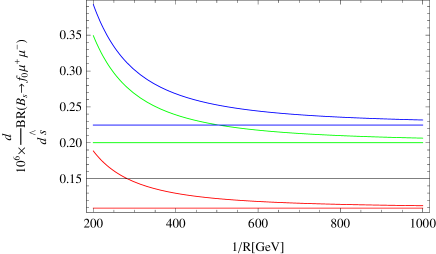
Figure 1: Dependence of the branching ratio on the $1/R$ for muon channel at three fixed values of the $\hat{s}$. The blue, green and red lines belong to the values $\hat{s}=0.2$, $\hat{s}=0.3$ and $\hat{s}=0.5$, respectively. The straight line shows the result of SM and the curve depicts the ACD model prediction in each case.

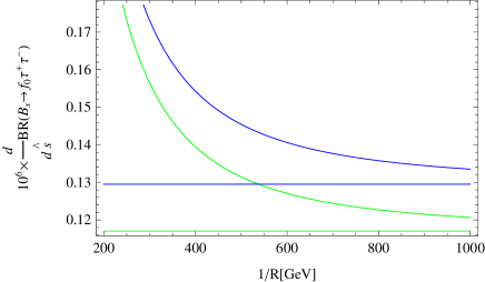
Figure 2: Dependence of the branching ratio on the $1/R$ for tau channel at two fixed values of the $\hat{s}$. The blue and green lines belong to the values $\hat{s}=0.5$ and $\hat{s}=0.6$, respectively. The straight line shows the result of SM and the curve depicts the ACD model prediction in each case.

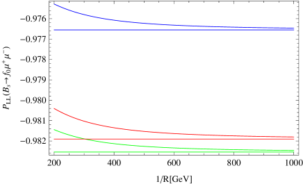
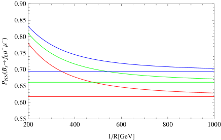
Figure 3: Dependence of the $P_{LL}$ and $P_{NN}$ on the $1/R$ for muon channel at three fixed values of the $\hat{s}$. The blue, green and red lines belong to the values $\hat{s}=0.2$, $\hat{s}=0.3$ and $\hat{s}=0.5$, respectively. The straight line shows the result of SM and the curve depicts the ACD model prediction in each case.

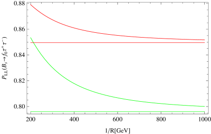
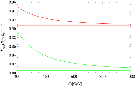
Figure 4: Dependence of the $P_{LL}$ and $P_{NN}$ on the $1/R$ for tau channel at two fixed values of the $\hat{s}$. The green and red lines belong to the values $\hat{s}=0.5$ and $\hat{s}=0.6$, respectively. The straight line shows the result of SM and the curve depicts the ACD model prediction in each case.

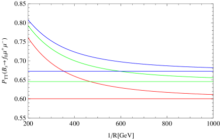
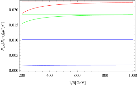
Figure 5: The same as FIG. 3 but for $P_{TT}$ and $P_{LN}$.

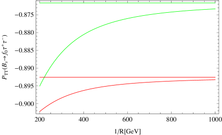
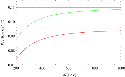
Figure 6: The same as FIG. 4 but for $P_{TT}$ and $P_{LN}$.

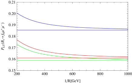
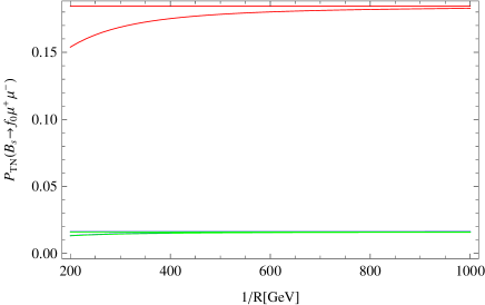
Figure 7: The same as FIG. 3 but for $P_{LT}$ and $P_{TN}$.

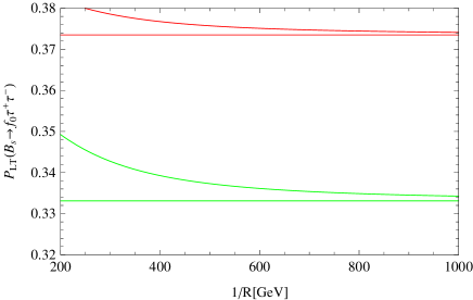
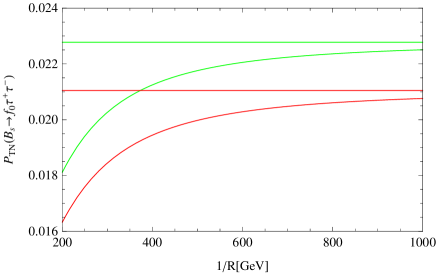
Figure 8: The same as FIG. 4 but for $P_{LT}$ and $P_{TN}$.

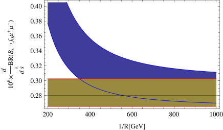
Figure 9: Dependence of the branching ratio on the $1/R$ for muon channel at $\hat{s}=0.2$ when errors of the form factors are taken into account. The straight band shows result of the SM and the curve band refers to the ACD model prediction.

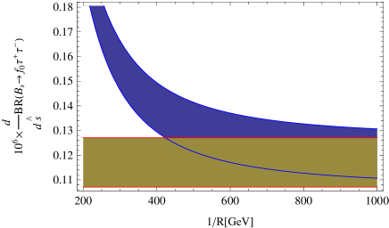
Figure 10: Dependence of the branching ratio on the $1/R$ for tau channel at $\hat{s}=0.6$ when errors of the form factors are taken into account. The straight band shows result of the SM and the curve band refers to the ACD model prediction.

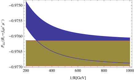
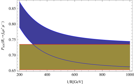
Figure 11: Dependence of the $P_{LL}$ and $P_{NN}$ on the $1/R$ for muon channel at $\hat{s}=0.2$ when errors of the form factors are taken into account. The straight bands show results of the SM and the curve bands refer to the the ACD model predictions.

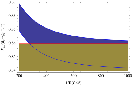
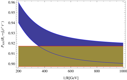
Figure 12: Dependence of the $P_{LL}$ and $P_{NN}$ on the $1/R$ for tau channel at $\hat{s}=0.6$ when errors of the form factors are taken into account. The straight bands show results of SM and the curve bands refer to the ACD model predictions.

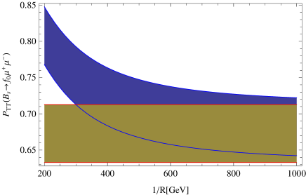
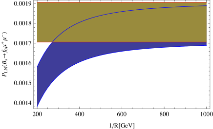
Figure 13: The same as FIG. 11 but for $P_{TT}$ and $P_{LN}$.

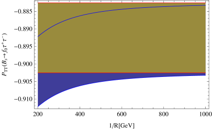
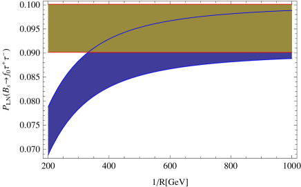
Figure 14: The same as FIG. 12 but for $P_{TT}$ and $P_{LN}$.

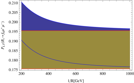
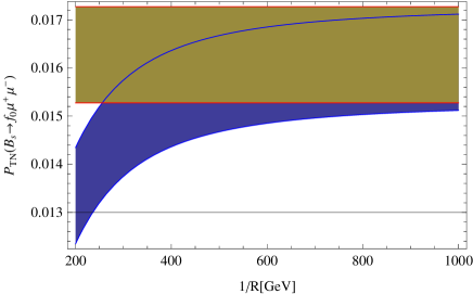
Figure 15: The same as FIG. 11 but for $P_{LT}$ and $P_{TN}$.

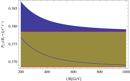
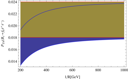
Figure 16: The same as FIG. 12 but for $P_{LT}$ and $P_{TN}$.

From these figures, we obtain the following results:

• There are considerable discrepancies between the results of the UED and SM predictions at lower values of the compactification factor for all observables and both lepton channels. When $1/R$ is increased, the differences between the predictions of two models become small so that two models have approximately the same predictions at $1/R=1000~{}GeV$.

• As it is expected, the branching ratio in $\tau$ channel is small comparing to that of the $\mu$.

• An increase in the value of $\hat{s}$ ends up in a decrease in the value of the differential branching ratio.

• The deviations of the UED results from those of the SM on double lepton polarization asymmetries are small in comparison with the deviation of the differential branching ratios from corresponding SM values. However these can not be overlooked.

• The contributions of KK modes enhance the absolute values of the $P_{LL}$ for $\tau$ as well as the $P_{NN}$, $P_{TT}$ and $P_{LT}$ for both lepton channels, but they decrease the absolute values of the $P_{LL}$ for $\mu$ and $P_{LN}$ and $P_{TN}$ for both leptons.

• The $P_{LL}$ for $\mu$ and $P_{TT}$ for $\tau$ have negative signs but the rest of double lepton polarization asymmetries have positive signs.

Now, we would like to discuss how the uncertainties of the form factors affect the physical quantities under consideration. For this aim, we plot the aforementioned physical observables on the compactification factor in figures 9-16 when the uncertainties of the form factors are taken into account. These figures are plotted at $\hat{s}=0.2$ and $\hat{s}=0.6$ for the $\mu$ and $\tau$ channels, respectively. From figures 9 and 10 for the branching fractions, it is clear that the difference between the UED and SM models predictions exist and can not be killed by uncertainties of the form factors especially at lower values of the compactification factor. The figures 11-16 for double lepton polarization asymmetries also depict that except the $P_{TT}$ and $P_{TN}$ in $\tau$ channel and $P_{LT}$ in both lepton channels, there are discrepancies between two model predictions at lower values of the $1/R$ even if the errors of the form factors are encountered.

In conclusion, making use of the related form factors calculated via light-cone QCD sum rules up to next-to-leading order corrections in $\alpha_{s}$, we analyzed the sensitivity of the differential branching ratio and various double lepton polarization asymmetries on the compactification factor of extra dimension for the $B_{s}\rightarrow f_{0}(980)\ell^{+}\ell^{-}$ transition. Our numerical calculations depict considerable deviations of the extra dimension model results from the SM predictions. These differences can not be killed by errors of the form factors in the allowed regions of the compactification parameter previously discussed. Such discrepancies can be interpreted as signals for existing extra dimensions in nature which can be searched for at hadron colliders. As a final note it is worth to estimate the accessibility to measure the branching ratio and lepton polarization asymmetries. An observation of a $3~{}\sigma$ signal for asymmetry of the order of the $1\%$ needs about $\sim 10^{12}$ $\bar{B}B$ pairs. This allow us to measure the branching ratio and the polarization asymmetries shown in the figures (1)-(16) in principle. The order of branching ratios show that the $B_{s}\rightarrow f_{0}(980)\ell^{+}\ell^{-}$ decay channel both for $\mu$ and $\tau$ leptons can be detected at LHC. However, as experimentalists say, there are some technical difficulties to measure the lepton polarizations. In the case of $\mu$, this lepton should be stopped in order to measure its polarizations which is not yet possible experimentally. For $\tau$ lepton, we should reconstruct then analyze the decay products of this lepton. In this case, we face with the problem of the efficiency of the reconstruction. If these technical difficulties over come, by measuring the considered double–lepton polarization asymmetries, we can get valuable information about the nature of interactions included in the effective Hamiltonian because as the large parts of the uncertainties are canceled out, the ratio of physical observables such as CP, forward–backward asymmetry and single or double–lepton polarization asymmetries less suffer from the uncertainty of the form factors compared to the branching ratio.

IV Acknowledgment

We would like to thank T. M. Aliev for his useful discussions.

References

• (1) P. Colangelo, F. De Fazio, R. Ferrandes and T. N. Pham, Phys. Rev. D 77, 055019 (2008).
• (2) M. V. Carlucci, P. Colangelo and F. De Fazio, Phys. Rev. D 80, 055023 (2009).
• (3) T. Appelquist, H. C. Cheng and B. A. Dobrescu, Phys. Rev. D 64, 035002 (2001).
• (4) I. Antoniadis, Phys. Lett. B 246, 377 (1990).
• (5) I. Antoniadis, N. Arkani-Hamed, S. Dimopoulos and G. Dvali, Phys. Lett. B 439, 257 (1998).
• (6) N. Arkani-Hamed, S. Dimopoulos and G. Dvali, Phys. Lett. B 429, 263 (1998); Phys. Rev. D 59, 086004 (1999).
• (7) D. Hooper, S. Profumo, Phys.Rept. 453 (2007) 29.
• (8) P. Colangelo, F. De Fazio, R. Ferrandes, T. N. Pham, Phys. Rev. D 73 (2006) 115006.
• (9) Yu-Ming Wang, M. Jamil Aslam, Cai-Dian Lu, Eur. Phys. J. C 59, 847 (2009).
• (10) T. M. Aliev, M. SavcΔ±, Eur. Phys. J. C 50, 91 (2007).
• (11) F. De Fazio, Nucl. Phys. Proc. Suppl. 174, 185 (2007).
• (12) B. B. Sirvanli, K. Azizi, Y. Ipekoglu, JHEP 1101, 069 (2011).
• (13) K. Azizi, N. KatΔ±rcΔ±, JHEP 1101, 087 (2011).
• (14) T. Appelquist, H. U. Yee, Phys. Rev. D 67, 055002 (2003).
• (15) V. Bashiry, M. Bayar, K. Azizi, Phys. Rev. D 78, 035010 (2008).
• (16) T. M. Aliev, M. Savci, B. B. Sirvanli, Eur. Phys. J. C 52, 375 (2007).
• (17) I. Ahmed, M. A. Paracha, M. J. Aslam, Eur. Phys. J. C 54, 591 (2008).
• (18) N. KatΔ±rcΔ±, K. Azizi, JHEP 1107, 043 (2011).
• (19) P. Colangelo, F. De Fazio, R. Ferrandes, T. N. Pham, Phys. Rev. D 74 (2006) 115006.
• (20) R. Mohanta and A. K. Giri, Phys.Rev. D 75 (2007) 035008.
• (21) U.Β Haisch and A.Β Weiler, Phys.Β Rev.Β D 76, 034014 (2007).
• (22) A.Β J.Β Buras, M.Β Spranger and A.Β Weiler, Nucl.Β Phys.Β B 660, 225 (2003).
• (23) A. J. Buras, A. Poschenrieder, M. Spranger Nucl. Phys. B D 678, 455 (2004).
• (24) A. Buras, M. Misiak, M. MΓΌnz and S. Pokorski, Nucl. Phys. B 424, 374 (1994).
• (25) M. Misiak, Nucl. Phys. B 393, 23 (1993); Erratum ibid B 439, 161 (1995).
• (26) B. Buras, M. MΓΌnz, Phys. Rev. D 52, 186 (1995).
• (27) K. Agashe, N. G. Deshpande, G. H. Wu, Phys. Lett. B 514 (2001) 309; B 511 (2001) 85; T. Appelquist, B. A. Dobrescu, Phys. Lett. B 516 (2001) 85.
• (28) I.Β Gogoladze and C.Β Macesanu, Phys.Β Rev.Β D 74, 093012 (2006).
• (29) J.Β A.Β R.Β Cembranos, J.Β L.Β Feng and L.Β E.Β Strigari, Phys.Β Rev.Β D 75, 036004 (2007).
• (30) G. Buchalla, A. J. Buras, M. E. Lautenbacher, Rev. Mod. Phys. 68, 1125 (1996).
• (31) M. Beneke, G. Buchalla, M. Neubert, C.T. Sachrajda, Eur. Phys. J. C 61 (2009) 439.
• (32) A. Khodjamirian, Th. Mannel, A.A. Pivovarov, Y.-M. Wang, JHEP 1009 (2010) 089.
• (33) P. Colangelo, F. De Fazio, W. Wang, Phys. Rev.D 81, 074001 (2010).
• (34) T. M. Aliev, V. Bashiry, M. Savci, Eur .Phys. J. C 35 (2004) 197.
• (35) V. Bashiry, S. M. Zeberjad, F. Falahati, K. Azizi, J. Phys. G 35, 065005 (2008) .
• (36) S. Fukae, C.S. Kim, T. Yoshikawa, Phys. Rev. D 61 (2000) 074015.