The Source Density and Observability of Pair-Instability Supernovae from the First Stars

Abstract

Theoretical models predict that some of the first stars ended their lives as extremely energetic pair-instability supernovae (PISNe). With energies approaching $10^{53}$ ergs, these supernovae are expected to be within the detection limits of the upcoming James Webb Space Telescope (JWST), allowing observational constraints to be placed on the properties of the first stars. We estimate the source density of PISNe using a semi-analytic halo mass function based approach, accounting for the effects of feedback from star formation on the PISN rate using cosmological simulations. We estimate an upper limit of $\sim$0.2 PISNe per JWST field of view at any given time. Feedback can reduce this rate significantly, e.g., lowering it to as little as one PISN per 4000 JWST fields of view for the most pessimistic explosion models. We also find that the main obstacle to observing PISNe from the first stars is their scarcity, not their faintness; exposures longer than a few times $10^{4}\,$s will do little to increase the number of PISNe found. Given this we suggest a mosaic style search strategy for detecting PISNe from the first stars. Even rather high redshift PISNe are unlikely to be missed by moderate exposures, and a large number of pointings will be required to ensure a detection.

1. Introduction

Understanding the formation of the first stars and galaxies is one of the central challenges of modern cosmology, as they mark a significant increase in complexity from the simple initial conditions of the primordial universe during the ‘dark ages’ (e.g., Barkana & Loeb 2001; Miralda-Escudé 2003; Bromm et al. 2009; Loeb 2010). The basic properties of these so-called Population III (Pop III) stars have been reasonably well established, with the consensus that the first stars formed in dark matter ‘minihalos’ on the order of $10^{5}$–$10^{6}$$\,{\rm M}_{\odot}$ at high redshifts (Couchman & Rees, 1986; Haiman et al., 1996; Tegmark et al., 1997). Numerical simulations of the collapse of primordial metal-free gas into these halos, where molecular hydrogen is the only available coolant, had suggested that the first stars were predominantly very massive, with $M_{*}\gtrsim 100$$\,{\rm M}_{\odot}$ and a top-heavy initial mass function (IMF) (e.g., Bromm et al. 1999, 2002; Abel et al. 2002; Bromm & Larson 2004; Yoshida et al. 2006; O’Shea & Norman 2007). More recent work has found that the gas from which the first stars formed underwent significant fragmentation (Stacy et al., 2010; Clark et al., 2011; Greif et al., 2011, 2012), and experienced strong protostellar feedback (Hosokawa et al., 2011; Stacy et al., 2012). These results have revised our picture of Pop III star formation, with lower characteristic masses (on the order of 50 rather than $100$$\,{\rm M}_{\odot}$) and a much broader IMF now expected. The light from these stars ended the dark ages and fundamentally transformed the universe, beginning both the reionization (e.g, Meiksin 2009) and the chemical enrichment of the universe (e.g, Karlsson et al. 2011).

Given the top-heavy nature of Pop III star formation and the fact that low-metallicity stars are unlikely to undergo significant radiatively driven mass loss (Kudritzki, 2002), one interesting possibility is that some of the first stars died as pair-instability supernovae (PISNe), a scenario that has significant consequences for the chemical enrichment history of the universe (Heger & Woosley, 2002; Tumlinson et al., 2004; Karlsson et al., 2008). Basic one-dimensional models predict that stars with masses in the range 140–260$\,{\rm M}_{\odot}$ will undergo a pair-production instability and explode completely (Barkat et al., 1967; Fraley, 1968). During core oxygen burning, a combination of high temperatures and relatively low densities results in the formation of $e^{\pm}$ pairs, removing pressure support from the core. Following the subsequent contraction, the ignition of explosive oxygen burning completely disrupts the progenitor, resulting in a significant contribution to the metal enrichment of the surrounding medium. More recently, Chatzopoulos & Wheeler (2012) and Yoon et al. (2012) have found that stars with initial masses as low as 65$\,{\rm M}_{\odot}$ can encounter the pair-production instability if they are rapidly rotating. In this scenario, strong rotationally induced mixing causes nearly homogeneous evolution, such that the star is converted almost entirely to helium before the next phase in its evolution begins. These extremely energetic explosions—approaching $10^{53}$ ergs for the most massive models—are very luminous, in part due to the large amount of ⁵⁶Ni produced, and are also very temporally extended as a result of the large mass ejected (Fryer et al., 2001; Heger & Woosley, 2002; Heger et al., 2003; Joggerst & Whalen, 2011; Kasen et al., 2011).

A second possiblility for reaching such extreme explosion energies in slightly lower mass stars is the hypernova scenario for rapidly rotating stars that undergo core collapse (Umeda & Nomoto, 2003; Tominaga et al., 2007). During the collapse, accretion onto a central black hole powers a jet which induces a highly energetic explosion. While recent work has decreased the expected mass of the first stars, they have also been found to rotate more rapidly than previously thought (Stacy et al., 2011), increasing the plausibility of this scenario. Evidence supporting this hypothesis has recently been presented by Chiappini et al. (2011).

While not an example of a Pop III star, the recent discovery of the extremely luminous supernova (SN) 2007bi, identified as a possible PISN, in a metal-poor dwarf galaxy at a redshift of $z\simeq 0.1$ (Gal-Yam et al., 2009) suggests that PISNe may be possible in the local universe under rare circumstances. Further supporting this picture, Woosley et al. (2007) have shown that SN 2006gy (Smith et al., 2007) is well modeled by a pulsational pair-instability model. For stars with initial masses in the range $\sim$100–140$\,{\rm M}_{\odot}$, the star encounters the $e^{\pm}$ production instability, but the resulting explosive ignition of oxygen is insufficient to unbind the star. Instead it ejects a shell of material before settling back into a stable configuration. The star encounters this instability several times until the mass of the helium core drops below $\sim$40$\,{\rm M}_{\odot}$, after which the star can proceed to silicon burning and eventually undergo core-collapse.

With the upcoming launch of the James Webb Space Telescope (JWST) we will be able to probe the epoch of first light in unprecedented detail. While the first stars themselves are unlikely to be visible (e.g, Bromm et al. 2001; Pawlik et al. 2011), some of the SNe that end their lives should be within the detection limits of the JWST (e.g., Mackey et al. 2003; Scannapieco et al. 2005; Gardner et al. 2006). While the basic properties of PISNe and the effect they have on their environment has been well studied (Mori et al., 2002; Bromm et al., 2003; Furlanetto & Loeb, 2003; Kitayama & Yoshida, 2005; Whalen et al., 2008; Wise & Abel, 2008; Greif et al., 2010), the source density of these events has yet to be well constrained.

The first attempt at estimating the number and observability of SNe at high redshift was made by Miralda-Escudé & Rees (1997), who calculated the all-sky SN rate based on estimates of the total metals produced by a typical SN and the observed metallicity of the intergalactic medium (IGM) at high redshifts. This yields $\sim$1 SN yr^-1 arcmin^-2 at $z\sim 5$. Other early work attempted to model the SN rate based on the empirically determined star formation rate out to high redshifts ($z\sim 5$; e.g., Madau et al. 1998; Dahlén & Fransson 1999). It should be noted that these attempts focused on Type II SNe, not PISNe, which are the focus of the present work. Mackey et al. (2003) estimated the PISN rate based on their calculations of the Pop III star formation rate, predicting $\sim$$2\times 10^{6}$ PISNe yr^-1 over the whole sky above $z=15$. Weinmann & Lilly (2005) performed a similar analysis with more conservative estimates for the star formation rate, finding a PISN rate of $\sim$4 yr^-1 deg^-2 above $z=15$ and $\sim$0.2 yr^-1 deg^-2 above $z=25$, as well as concluding that PISNe should be observable out to $z=50$ with the JWST.

Subsequent work by Wise & Abel (2005) determined the PISN rate based on the collapse of gas into dark matter minihalos. Accounting for radiative feedback, they concluded that $\sim$0.34 PISNe yr^-1 deg^-2 were to be expected above $z=10$, as well as briefly considering the detectability of PISNe at high redshifts based on models from Heger & Woosley (2002). Scannapieco et al. (2005) presented a more thorough analysis of the visibility of PISNe based on a suite of numerical simulations spanning the range of theoretical PISN models using the implicit hydrodynamics code KEPLER. Mesinger et al. (2006b) presented a similar but more general halo mass function based analysis, considering the rates and detectability of all SNe; they briefly consider primordial PISNe, but focus on core-collapse SNe and their detectability. More recently, Trenti et al. (2009) explored the observable PISN rate within the context of the metal-free gas supply during the epoch of reionization.

Our work improves upon these investigations by incorporating updated PISN models from Kasen et al. (2011) and determining their observability using the published specifications of the Near Infrared Camera (NIRcam) on the JWST. In the final stages of the work on this paper we have become aware of the study by Pan et al. (2012), who have performed a similar analysis. This paper addresses the question of PISN observability in a nicely complementary way by employing a different normalization strategy. Different from our assumption that viable Pop III progenitors can only form in unenriched minihalos at $z\gtrsim 6$, Pan et al. (2012) derive the star formation rates required to produce sufficient photons for reionization. They then infer the PISN rate corresponding to different choices for the IMF. Their analysis is thus able to probe the charachter of star formation in the dwarf galaxies that are the main drivers of reionization, whereas we focus on the minihalos where Pop III stars first begin to form.

This paper is organized as follows. In Section 2 we describe our semi-analytic model for the PISN rate. We consider the ability of the JWST to detect PISNe at high redshift in Section 3, and our conclusions are gathered in Section 4. Throughout this paper we adopt a $\Lambda$CDM model of hierarchical structure formation, using cosmological parameters consistent with the WMAP 5-year results (Komatsu et al., 2009): $\Omega_{\rm m}=0.258$; $\Omega_{\Lambda}=0.742$; $\Omega_{b}=0.0441$; $h=0.719$; $n_{s}=0.96$; $\sigma_{8}=0.796$.

2. The PISN Rate

PISNe are produced only by very massive stars (Bromm et al., 2001; Schaerer, 2002; Heger et al., 2003), which are now expected to be rare even for Pop III star formation. After the first massive star forms, the resulting heating from photoionization quickly suppresses the density of the remaining gas in the minihalo, effectively halting star formation (Kitayama et al., 2004; Whalen et al., 2004; Alvarez et al., 2006). The energy released by the first PISN disperses the gas in the halo and contaminates it with metals (Bromm et al., 2003; Greif et al., 2007; Whalen et al., 2008; Wise & Abel, 2008; Greif et al., 2010). Subsequent episodes of star formation are thus delayed until the gas is able to recondense into more massive cosmological halos (Yoshida et al., 2004, 2007; Johnson et al., 2007; Alvarez et al., 2009). While star formation will resume at this point, the gas in these systems is expected to be enriched beyond the critical metallicity for the transition to Population II (Pop II) star formation (Wise & Abel, 2007, 2008; Greif et al., 2007, 2008, 2010). As a result, the stars that form will no longer be massive enough to reliably produce PISNe. These explosions are thus only expected to occur in minihalos containing pristine gas that has just crossed the density threshold for star formation via H₂ cooling, and only one PISN occurs per halo.

It is possible that the first stars formed in binaries or small multiples; however, the number of massive stars formed per minihalo is still of order unity (Stacy et al., 2010; Clark et al., 2011; Greif et al., 2011). Given this, and assuming that the time required for the progenitor star to form, live and die is negligible (Heger et al., 2003), we can use the formation rate of minihalos to place a robust upper limit on the PISN rate.

The introduction of cosmic feedback has the potential to significantly alter this picture. Chemical enrichment induces a transition to lower mass Pop II star fomation, and thus always has a negative effect on the PISN rate. Radiative feedback—especially $\mathrm{H}_{2}$-dissociating Lyman-Werner (LW) feedback—has a more complicated effect. The destruction of molecular hydrogen by LW photons removes the ability of pristine gas to cool effectively. This suppresses star formation, and hence negatively affects the PISN rate. However this merely delays star formation; as the halo mass continues to increase, the gas eventually becomes self-shielding and proceeds with cooling and collapse. The delay effectively increases the amount of gas available when star formation begins. This increases the possibility of multiple massive stars forming simultaneously, positively affecting the PISN rate. To account for these possibilities, we consider three scenarios. First we estimate the PISN rate assuming that the first stars form unimpeded by cosmic feedback. Then we consider a conservative scenario in which both chemical and LW feedback affect the PISN rate, but only one star forms per halo. Finally, we allow for enhanced massive star formation in the LW-affected halos, and calculate the observable rate for each scenario.

2.1. No-Feedback Limit

In order to determine an upper limit to the PISN rate, we assume exactly one PISN per minihalo, forming as soon as the virial temperature of the minihalo exceeds the minimum value $T_{\rm crit}$ required for gas to cool and collapse to high densities. We set this to 2200 K based on the results of simulations (see § 2.2.1 for details). The corresponding critical mass for collapse is given by

$$M_{\rm crit}=10^{6}\,{\rm M}_{\odot}\left(\frac{T_{\rm crit}}{10^{3}\,{\rm K}}\right)^{3/2}\left(\frac{1+z}{10}\right)^{-3/2},$$ (1)

where we assume a mean molecular weight of $\mu=1.22$, appropriate for the almost completely neutral IGM at high redshifts (Barkana & Loeb, 2001).

We use the analytic Press-Schechter (PS) formalism for structure formation (Press & Schechter, 1974) to estimate the number density $n_{\textsc{ps}}$ of minihalos of mass $M$ at redshift $z$, given by

$$n_{\textsc{ps}}(M,z)=\sqrt{\frac{2}{\pi}}\frac{\rho_{\rm m}}{M}\left|\frac{d\ln\,\sigma_{0}(M)}{d\ln\,M}\right|\nu_{c,z}\,e^{-\nu_{c,z}^{2}/2},$$ (2)

where $\rho_{\rm m}$ is the background matter density, $\sigma_{z}(M)$ is the standard deviation of overdensities $\delta$ of mass $M$ at redshift $z$, and $\nu_{c,z}=\delta_{c}/\sigma_{z}(M)$, where $\delta_{c}$ is the critical overdensity for collapse; the value used here is $\delta_{c}=1.686$.

Converting from redshift to cosmic time $t(z)$, where

$$t(z)=\frac{1}{H_{0}}\int_{z}^{\infty}\frac{dz^{\prime}}{(1+z^{\prime})\sqrt{\Omega_{\rm m}(1+z^{\prime})^{3}+\Omega_{\Lambda}}},$$ (3)

a first order estimate for the PISN formation rate as a function of redshift is given by $\dot{n}_{\textsc{pisn}}\equiv dn_{\textsc{ps}}/dt$. However, this estimate is only valid while the rate of destruction of minihalos via mergers remains small compared to the formation rate. The Press-Schechter formalism only gives the total number of halos of a given mass at a given redshift. As a result, once mergers become important the rate of change of the total number of minihalos no longer traces the formation rate. To correct for this, we use the expression for the formation rate derived by Sasaki (1994):

$$\dot{n}_{+}(z)=\frac{\dot{D}}{D}n_{\textsc{ps}}(M_{\rm crit},z)\frac{\delta_{c}^{2}}{\sigma^{2}_{0}(M)D^{2}},$$ (4)

where $D(z)$ is the growth factor. The PISN rate in this upper limit of no feedback, shown in Figure 2 (blue line), is then simply given by the halo formation rate:

$$\dot{n}_{\textsc{pisn}}(z)=\dot{n}_{+}(z).$$ (5)

2.2. Feedback

The preceding analysis has only nominally incorporated the baryonic physics involved through the critical mass for H₂ cooling. Gas will not successfully cool and collapse in all minihalos that reach the critical mass (e.g., Yoshida et al. 2003). The various feedback mechanisms responsible for this include photoheating from stars in nearby halos and the buildup of a background of H₂ dissociating LW photons. Chemical feedback will enrich the gas with metals, improving its ability to cool. However, gas that is enriched forms lower-mass Pop II stars, effectively reducing the PISN rate. These feedback mechanisms can be represented with distinct efficiency factors $\eta(z)$, such that the true PISN rate will be given by

$$\dot{n}_{\textsc{pisn}}(z)=\eta_{\rm chem}(z)\;\eta_{\rm rad}(z)\;\dot{n}_{+}(z).$$ (6)

We must include these effects in order to derive a realistic estimate for the PISN rate, which we henceforth refer to as the conservative feedback case.

2.2.1 Lyman-Werner Feedback

LW feedback is of particular importance in any discussion of feedback on the first stars as it dissociates the H₂ molecules primarily responsible for cooling primordial gas. This significantly reduces the ability of the gas to cool and works to suppress further star formation (Haiman et al., 1997; Omukai & Nishi, 1999; Ciardi et al., 2000; Haiman et al., 2000; Glover & Brand, 2001; Kitayama et al., 2001; Machacek et al., 2001; Ricotti et al., 2001, 2002a, 2002b; Yoshida et al., 2003; Omukai & Yoshii, 2003; Mesinger et al., 2006a). As the first stars form in $\gtrsim 3\sigma$ peaks in the Gaussian distribution of density fluctuations (Barkana & Loeb, 2001), we focus here on a similarly overdense environment in order to provide a conservative estimate of the effects of LW feedback on the PISN rate. While representative of the LW background in Pop III star formation sites, this is likely not representative of the ‘average’ LW background in the universe (e.g., Machacek et al. 2001; Mesinger et al. 2006a).

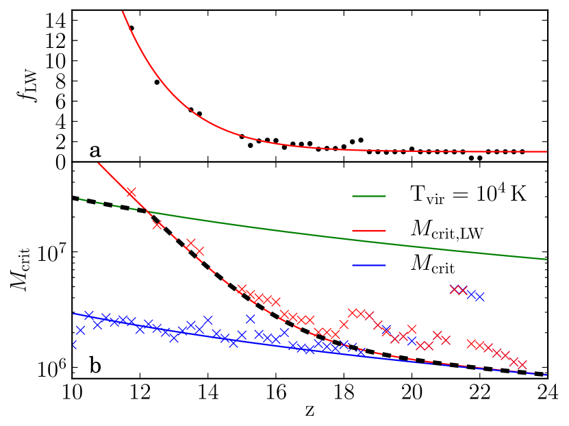
Figure 1.— a) the factor $f_{\textsc{lw}}$ by which LW feedback increases the critical mass for star formation; points show the results of the simulation, the red line our fit. b) The critical mass for star formation in both simulations. Blue crosses mark the critical mass for star formation in the absence of LW feedback, red crosses in its presence. The blue line shows the best fit critical mass from Equation 1, given by a temperature of 2200 K; the red line the critical mass from Equation 9 for LW feedback using the fit for $f_{\textsc{lw}}$ given in Equation 8. The green line marks the halo mass corresponding to a virial temperature of $10^{4}\,$K, and the black dashed line represents the critical mass employed, accounting for atomic cooling in halos with virial temperatures above $10^{4}\,$K.

We will describe our radiative feedback simulations in detail elsewhere, and present only a brief summary here. We employ a set of two cosmological simulations using a modified version of the $N$-Body/TreePM SPH code GADGET (Springel, 2005; Springel et al., 2001) to gauge the effects of LW feedback on the PISN rate. These simulations, carried out in a box of size $3.125\,h^{-1}$ comoving Mpc and starting from a redshift of $z=127$, were performed to investigate the formation of the first dwarf galaxies in $10^{9}$$\,{\rm M}_{\odot}$ halos at $z=10$. In order to obtain high resolution in the halo containing the first galaxy while retaining information about structure on large scales, a zoomed simulation technique was used, with the highest resolution dark matter (gas) particles having a mass of 2350 (484)$\,{\rm M}_{\odot}$. This allows halos with masses $\gtrsim 2\times 10^{5}$$\,{\rm M}_{\odot}$, to be resolved with $\gtrsim 100$ dark matter particles.

The first of the simulations we employ is similar to simulation Z4 presented in Pawlik et al. (2011), and follows the non-equilibrium chemistry and cooling of the primordial atomic and molecular gas, including star formation but not the associated feedback. It thus provides a useful reference against which the effects of LW feedback can be discussed. Here, gas particles were turned stochastically into star particles at densities $n_{\rm H}>500\,{\rm cm}^{-3}$ on a dynamical time scale. Star particles were considered simple stellar populations using the zero-metallicity top-heavy IMF models from Schaerer (2003). Henceforth this simulation is referred to as Simulation A.

The second simulation employed here, which we refer to as Simulation B, is identical to Simulation A except for the inclusion of LW feedback. Calculation of the feedback was carried out by considering the contribution from both star particles and a uniform LW background. The combined LW background is normalized to approximate the LW background evolution shown in Greif & Bromm (2006) in the optically thin limit, but with the application of a self-shielding correction (Wolcott-Green et al., 2011).

The efficiency of LW feedback, $\eta_{\textsc{lw}}$, can be expressed as the ratio of the formation rate of minihalos at the critical mass with LW feedback to that without:

$$\eta_{\textsc{lw}}(z)=\frac{\dot{n}_{+}(M_{\rm crit,\textsc{lw}},z)}{\dot{n}_{+}(M_{\rm crit},z)}.$$ (7)

This requires determining the factor $f_{\textsc{lw}}(z)$ by which LW feedback increases the critical mass for star formation. We do this by determining the critical mass required for stars to form in both simulations, as traced by the lowest mass halo that is actively forming stars for the first time. The resulting critical mass in each case is shown in Figure 1b; blue points denote the critical mass in Simulation A, red points in Simulation B. Without any negative feedback, we expect stars to form when the halo reaches the critical mass given in Equation 1. We find the that the resulting critical mass in Simulation A is best fit by a critical virial temperature of 2200 K, as shown in Figure 1b. Note that this includes the effects of dynamical heating; gas in isolated halos would collapse and form stars at lower masses.

Determining the critical mass for star formation in the LW feedback simulation in the same manner as above, we can then determine $f_{\textsc{lw}}$, shown in Figure 1a. We find that $f_{\textsc{lw}}$ is well fit by a functional form of

$$\begin{split}f_{\textsc{lw}}(z)=-6.23\times 10^{-5}\;&\textrm{erf}[0.094(z-0.204)]\\ &+6.23\times 10^{5},\end{split}$$ (8)

for $z\geq 10$, where ${\rm erf}(z)$ is the error function. $M_{\rm crit,\textsc{lw}}$ is then given by

$$M_{\rm crit,\textsc{lw}}=f_{\textsc{lw}}\,M_{\rm crit},$$ (9)

shown in Figure 1b. When the virial temperature of the halo reaches $10^{4}\,$K, cooling via atomic hydrogen becomes efficient and molecular hydrogen becomes unimportant. Once this threshold is reached, LW feedback cannot further suppress star formation, and $M_{\rm crit,\textsc{lw}}$ holds steady at a constant virial temperature of $10^{4}\,$K. This is reflected as an increase in the formation rate of halos affected only by LW feedback, as the formation rate of atomic cooling halos is increasing prior to $z=10$. This transition can be clearly seen in Figure 2, marked by a sudden jump in the halo formation rate. As ionizing photons cannot easily escape the immediate vicinity of the star that produced them, their impact on neighboring halos is small compared to that of LW photons at the highest redshifts. We thus set $\eta_{\rm rad}\simeq\eta_{\textsc{lw}}$ for simplicity. This approximation becomes increasingly unphysical close to the epoch of reionization at $z\sim 10$.

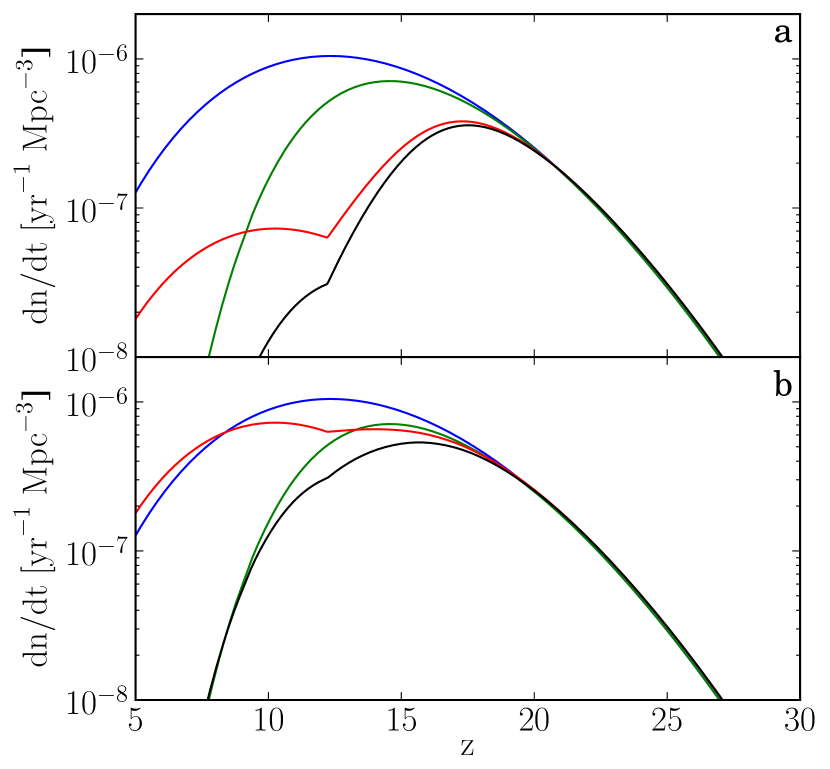
Figure 2.— a) $\dot{n}_{\textsc{pisn}}$ in the upper limit of no feedback (blue), with chemical feedback (green), LW feedback (red) and the resulting PISN rate for the conservative (chemical plus LW) feedback case (black). b) Same as (a), but for enhanced massive star formation.

2.2.2 Chemical Feedback

The process of chemical enrichment is another crucial factor for determining the PISN rate. Gas that has been enriched beyond a critical metallicity of $Z_{\rm crit}\sim 10^{-4}$$\,{\rm Z}_{\odot}$ will no longer form Pop III stars (Bromm et al., 2001; Schneider et al., 2002; Bromm & Loeb, 2003), and hence no PISNe. Chemical feedback can thus be represented as the fraction of halos forming from pristine gas at a given redshift. Realistic three-dimensional simulations of this process starting from cosmological initial conditions have become possible in the past decade, showing that enrichment by Pop III SNe, if they are highly energetic, proceeds very inhomogeneously, enriching the IGM before penetrating into denser regions (Scannapieco et al., 2005; Greif et al., 2007; Tornatore et al., 2007; Wise & Abel, 2008; Maio et al., 2010).

In modeling $\eta_{\rm chem}$, we use the results of Furlanetto & Loeb (2005). Their semi-analytic treatment of SN winds utilizes the Sedov (1959) solution for an explosion expanding into a uniform medium and yields a probability function $P_{\rm pristine}(z)$ that the gas in a newly formed halo is pristine. This is plotted in Figure 2 of their paper for various strengths of chemical feedback. We identify this quantity as the fraction of newly collapsed halos that have been polluted with metals, $\eta_{\rm chem}$. Given the recent detection of pristine gas at $z=3$ by Fumagalli et al. (2011), we choose the weakest feedback scenario presented by Furlanetto & Loeb (2005) among the scenarios that incorporate a clustering of sources. The resulting PISN rate is given by the green line in Figure 2.

2.3. Enhanced Massive Star Formation

Gas cooling and subsequent star formation in halos affected by LW feedback can be delayed until nearly an order of magnitude more gas is available for star formation (Figure 1). This increases the likelihood that multiple massive stars form per halo, offseting the negative effects of LW radiation considered above. We quantify this by positing that the number of PISNe produced per halo at redshift $z$ is given by the ratio of the critical mass in the presence of LW feedback $M_{\rm crit,\textsc{lw}}$ to the critical mass in the no-feedback case $M_{\rm crit}$. For example, at $z=17$, $M_{\rm crit,\textsc{lw}}/M_{\rm crit}\approx 1.4$, so for every 10 pristine halos that form, 14 PISNe are produced. In this case the PISN rate is modified such that

$$\dot{n}_{\textsc{pisn}}(z)=\frac{M_{\rm crit,\textsc{lw}}(z)}{M_{\rm crit}(z)}\;\eta_{\rm chem}(z)\;\eta_{\rm rad}(z)\;\dot{n}_{+}(z).$$ (10)

The resulting enhanced PISN rate can be seen in Figure 2b. In contrast to the conservative feedback case, the net effect of LW feedback is much less significant here, with chemical feedback controlling the final PISN rate.

2.4. The Observable Rate

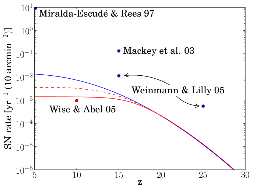
Figure 3.— The observable PISN rates in number per year per JWST field of view above a given redshift in the upper limit of no feedback (blue line), in the conservative feedback case (solid red line), and the enhanced star formation case (dashed red line). The rates calculated by Miralda-Escudé & Rees (1997), Mackey et al. (2003), Weinmann & Lilly (2005) and Wise & Abel (2005) are also shown for reference. Red points account for feedback; blue points do not.

The observed PISN rate per unit time per unit redshift per unit solid angle is given by

$$\begin{split}\frac{dN}{dt_{\rm obs}\,dz\,d\Omega}&=\frac{dN}{dt_{\rm obs}\,dV}\,\frac{dV}{dzd\Omega}\\ &=\frac{1}{(1+z)}\frac{dN}{dt_{\rm em}\,dV}\;r^{2}\frac{dr}{dz}.\end{split}$$ (11)

Cosmological time dilation between $t_{\rm obs}$ and $t_{\rm em}$ is accounted for by the $(1+z)$ in the denominator; $dV$ is the comoving volume element and $r(z)$ is the comoving distance to redshift $z$ given by

$$r(z)=\frac{c}{H_{0}}\int_{0}^{z}\frac{dz^{\prime}}{\sqrt{\Omega_{\rm m}(1+z^{\prime})^{3}+\Omega_{\Lambda}}},$$ (12)

where $c/H_{0}$ is the Hubble distance. With the assumptions outlined above, we estimate the PISN rate in events per year per comoving Mpc³ in the source rest frame:

$$\frac{dN}{dt_{\rm em}\,dV}=\dot{n}_{\textsc{pisn}}(z).$$ (13)

These results—shown in Figure 3—are in reasonable agreement with previous work; our no-feedback limit of one PISN per minihalo is somewhat more conservative than that employed by Weinmann & Lilly (2005), but in general agreement. Likewise, our conservative feedback rate is in good agreement with the rate found by Wise & Abel (2005), which also accounted for feedback. The discrepancy with the remaining rates can be attributed to the fact that Mackey et al. (2003) employed an optimistic star formation efficiency of $\eta_{*}=0.10$, while Miralda-Escudé & Rees (1997) performed a rough estimate of the all-sky supernova rate based on the observed metallicity of the IGM. This estimate of course includes Population I and II supernovae in addition to PISNe, and is included only for reference.

3. JWST Observability

While PISN explosions are predicted to be extremely energetic, the highest redshift events will still be unobservable, and those at lower redshifts will be above the detection limits of the JWST for only a fraction of their lifetimes. To determine the observability of these explosions we must consider both how bright they will be at a given redshift and how long they will remain visible. To span the uncertainties arising from variation in the progenitors of PISNe we consider a set of four models from Kasen et al. (2011), namely their R250, B200, R175 and He100 models. R250 and R175 are red supergiants of 250$\,{\rm M}_{\odot}$ and 175$\,{\rm M}_{\odot}$, respectively, spanning the mass range of succesful explosions. We also consider a more compact 200$\,{\rm M}_{\odot}$ blue supergiant (B200) and a 100$\,{\rm M}_{\odot}$ bare helium core (He100). All models considered here die as PISNe, with explosion energies ranging from $7\times 10^{52}$ ergs (R250) to $2\times 10^{52}$ ergs (R175). The late-time luminosity is powered by the decay of ⁵⁶Ni produced during the explosion. 40$\,{\rm M}_{\odot}$ of ⁵⁶Ni are produced in the R250 model, while only 5, 2 and 0.7$\,{\rm M}_{\odot}$ are produced in He100, B200 and R175, respectively.

Bare helium cores, such as the He100 model, are of particular interest in light of recent work finding that rapidly rotating stars can encounter the pair-production instability in progenitors with masses as low as 65$\,{\rm M}_{\odot}$ (Chatzopoulos & Wheeler, 2012; Yoon et al., 2012). Combined with recent work finding that Pop III stars are both less massive and more rapidly rotating than previously thought (Stacy et al., 2010, 2011, 2012; Clark et al., 2011; Greif et al., 2011, 2012), the explosion of a rapidly rotating helium core formed by homogeneous evolution represents an intriguing possibility.

We first describe our technique for fitting a blackbody to these four PISN models before considering their visibility with the JWST. We then estimate the total observable number in each case and for each feedback prescription. Finally, we briefly discuss the challenges involved in actually identifying PISNe as such.

3.1. A Simple Lightcurve Model

In order to determine how long a PISN will be visible we must model the source spectrum. Given the large mass involved, the ejecta will remain optically thick until late times, so we make the reasonable assumption that the PISN emits as a blackbody for the majority of its visible lifetime. Using the U, B, V, R, I, J, H, and K absolute magnitude light curves presented in Kasen et al. (2011), we perform a least-squares fit to find the combination of temperature $T$ and radius $R_{\textsc{sn}}$ that best matches the broadband magnitudes at each point in time. This is done with the assumption that the specific luminosity of the PISN $L_{\textsc{sn},\lambda}$ at wavelength $\lambda$ is given by

$$L_{\textsc{sn},\lambda}=4\pi^{2}R_{\textsc{sn}}^{2}B_{\lambda}(T),$$ (14)

where $B_{\lambda}$ is the Planck function. The resulting fits for the evolution of the temperature and radius of the PISN models are shown in Figure 4.

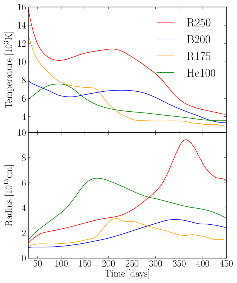
Figure 4.— The temperature and radius of our blackbody fits as a function of source frame time since the explosion for models R250, B200, R175 and He100. The secondary rise in temperature seen in R250 and B200 is caused by the decay of ⁵⁶Ni reheating the ejecta at late times. Note also that the apparent radii begin to decrease again at late times; this can be interpreted as the photosphere receding into the ejecta as the material cools.

Note that our blackbody assumption breaks down at late times when the photosphere begins to recede into the ejecta. This is manifested as an apparent decrease in the radius of the PISN remnant.

Figure 5.— Left: Lightcurves for the Kasen et al. (2011) R250 (top) and B200 (bottom) models as they would be observed by JWST’s F444W NIRCam filter at $z=5,10,15,20,25\>{\rm and}\>30$. The flux limits for a $10^{6}\,$s (dashed line) and $10^{4}\,$s (dotted line) exposure are shown for reference. Right: The visibility time $\Delta t_{\rm vis}$ in years for R250 (top) and B200 (bottom) as a function of redshift for each of the NIRcam wide filters. Note that the axes are scaled independently. Similar plots for models He100 and R175 are included in the appendix.

With this information we can then calculate the specific flux $F_{\lambda,\rm em}$ in the rest frame and—accounting for redshift and cosmological dimming—in the observer’s frame for a source at redshift $z$:

$$F_{\lambda,\rm obs}(T,R_{\textsc{sn}},z)=\pi\left[\frac{R_{\textsc{sn}}}{D_{L}(z)}\right]^{2}\frac{B_{\lambda^{\prime}}(T)}{1+z}.$$ (15)

Here $\lambda^{\prime}=\lambda/(1+z)$ accounts for redshifting, and the luminosity distance $D_{L}=(1+z)r(z)$ accounts for cosmological dimming. Convolving this spectrum with a filter function $\phi_{\textsc{x}}(\lambda)$ yields the observable flux in filter X:

$$F_{\rm obs,\textsc{x}}=\int_{0}^{\infty}\phi_{\textsc{x}}(\lambda)F_{\lambda,\rm obs}(T,R_{\textsc{sn}},z)d\lambda.$$ (16)

3.2. Visibility

The NIRCam instrument on the JWST will observe the early universe through a number of narrow, medium-width, and wide filters. The widest, longest-wavelength filter, F444W, will observe from 3.3 to 5.6 $\mu$m with a sensitivity limit of 24.5 nJy required for a $10\sigma$ detection in $10^{4}\,$seconds (Gardner et al., 2006). Shown in the left-hand column of Figure 5 is the observable flux as it would appear in the F444W NIRCam filter at various redshifts for the most and least easily observable models, R250 and B200, respectively. See Figure 7 for why these two were chosen; models He100 and R175 can be found in the appendix. The flux limits for the filter of $4.4\times 10^{-19}$ erg s^-1 cm^-2 for a $10^{6}\,$s exposure and $4.4\times 10^{-18}$ erg s^-1 cm^-2 for a $10^{4}\,$s exposure are also shown for reference. We see that the brightest explosions (R250) would be visible to beyond $z\sim 25$, but are never so bright as to be detectable with current generation telescopes. This is consistent with the non-detection by Frost et al. (2009) in a search of the Spitzer/IRAC Dark Field for possible Pop III PISN candidates.

To account for absorption of flux by neutral hydrogen along the line of sight we implement a simple model of instant reionization at $z=10$. For sources above this redshift, we assume no flux is observed shortward of the rest frame Ly$\alpha$ line. This is not relevant for the F444W NIRcam filter as Ly$\alpha$ does not redshift into the filter until $z\sim 40$, when the lightcurve is already far below even the $10^{6}\,$s sensitivity limit. It does however have an effect, albeit a small one, on the F115W and F090W filters.

At low redshifts the duration of the lightcurve presented in Kasen et al. (2011) is not quite long enough for the observed flux to reach the sensitivity limit; we extend it to the limit by extrapolating assuming a power-law scaling. The visible time $\Delta t_{\rm vis}$ is then simply given by the time the lightcurve is above the filter sensitivity limit. Shown in Figure 5 are the visibility times as a function of redshift for each of the NIRcam filters.

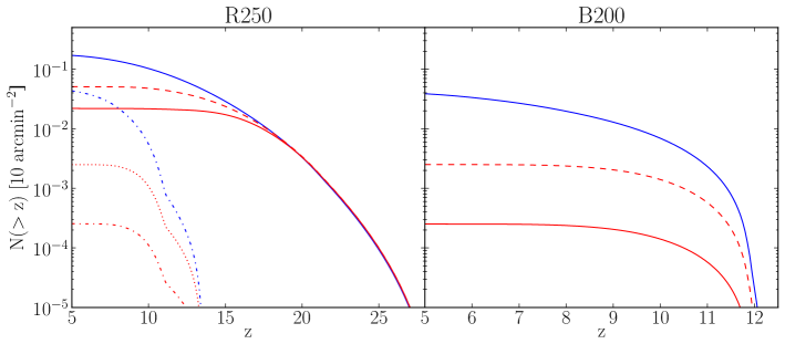
Figure 6.— Upper and lower limits for the number of PISNe per JWST FoV above redshift $z$ with different feedback prescriptions. The observable numbers for a $10^{6}\,$s exposure assuming the R250 model are shown on the left; the B200 model is employed on the right. Solid blue lines show an upper limit to the observable number in the case of no feedback, solid red lines an estimate for the observable number in our conservative feedback scenario, and dashed red lines the number in the enhanced star formation case. Note that the x-axis is scaled independently in each panel. Also shown in the R250 panel are the observable numbers for a $10^{4}\,$s exposure for the no-feedback (dot-dashed blue), conservative feedback (dot-dashed red), and enhanced star formation (dotted red) scenarios. The B200 model is not visible above $z=5$ in a $10^{4}\,$s exposure.

3.3. The Observable Number

With this estimate for $\Delta t_{\rm vis}$, we may finally calculate the observable number of PISNe on the sky, given by the product of the PISN rate at $z$, as seen in the observer frame, and the time a PISN at $z$ is visible, $\Delta t_{\rm vis}$. This yields an estimate for the number of PISNe visible on the sky at any given time per unit redshift per unit solid angle:

$$\frac{dN}{dz\,d\Omega}\simeq\frac{dN}{dt_{\rm obs}\,dz\,d\Omega}\,\Delta t_{\rm vis}.$$ (17)

Figure 6 shows the number of PISNe per JWST field of view (FoV) above redshift $z$ in a $10^{6}\,$s exposure for all three feedback cases for models R250 and B200. Models He100 and R175 can be found in the appendix. For the R250 model the results for a $10^{4}\,$s exposure are also included; B200 is not visible at high redshifts in a $10^{4}\,$s exposure.

In the optimistic case of an R250-type PISN with no feedback we expect $\sim$0.2 PISNe per JWST FoV for a $10^{6}\,$s exposure. In the most pessimistic case of a B200-type PISN with strong negative feedback this number drops to $\sim$2.5$\,\times 10^{-4}$ per FoV. The actual number detected by the JWST will most likely lie somewhere within this range. Given this, we conclude that a single deep pencil-beam survey is unadvisable for detecting PISNe, as there aren’t enough in a given field to ensure a detection, even in the most optimistic upper limit. This suggests that a mosaic search, covering a larger area with shorter exposure times, may be the best approach to ensure finding a Pop III PISN.

3.4. PISN Identification

The exceedingly long duration of their lightcurves poses a serious challenge for identifying PISNe. When combined with the cosmological time dilation factors involved, PISN lightcurves can last for decades; the highest redshift events will last longer than the projected mission lifetime for the JWST, making the detection of PISNe by searching for transients difficult at best. However, a multi-year campaign might be able to detect photometric variations; for example, the He100 model would appear to decline in brightness by $\sim$0.3 magnitudes per year at redshift $z=10$ (Kasen et al., 2011). Additionally, PISN colors become redder over time as the photosphere receeds into the ejecta and metal line blanketing suppresses flux in the bluer bands. While likely insufficient to unambiguously identify PISNe, this could be useful in selecting candidates for spectroscopic follow-up.

While the peak bolometric luminosities and spectra of PISNe resemble those of typical Type Ia and Type II supernovae (Joggerst & Whalen, 2011; Kasen et al., 2011), relatively little mixing occurs during the explosion (Joggerst & Whalen, 2011; Chen et al., 2011). As a result, PISNe mostly retain their onion-layer structure during the explosion, and metal lines do not appear in the spectrum until late times when the photosphere has receeded deep into the ejecta. Some lighter elements may appear, but the early spectrum of a PISN will be devoid of Si, Ni and Fe lines (Joggerst & Whalen, 2011). This may provide the spectroscopic signature needed to identify PISNe.

4. Discussion and Conclusions

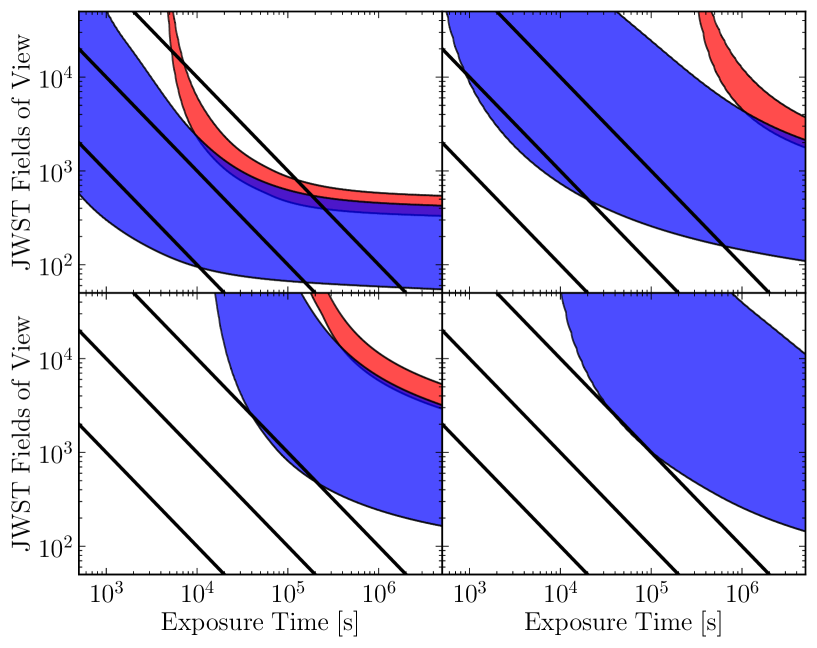
Figure 7.— The observability of the R250, He100, B200, and R175 models (clockwise from upper left) from Kasen et al. (2011) using the JWST’s NIRcam F444W filter. Shown is the possible range for the number of JWST FoVs required to detect 10 sources as a function of exposure time. The blue range is for all PISNe, and the red for PISNe from $z>15$. The lower boundaries correspond to the no-feedback upper limit to the PISN rate and the upper boundaries to the conservative feedback rate. From left to right, the black lines represent the number of pointings possible in a total of $10^{6}$, $10^{7}$, and $10^{8}\,$s for a given exposure time.

In this work, we have examined the source density of PISNe from Pop III stars and considered their detectability with the JWST. We conclude that the limiting factor in detecting PISNe will be the scarcity of sources rather than their faintness, in agreement with the conclusions of Weinmann & Lilly (2005). The brightest PISNe should be readily detectable with the longest wavelength NIRcam filters out to $z\sim 25$; the problem is the overall scarcity of sources.

We have derived an estimate for the observable PISN rate, finding an upper limit of just over 0.01 PISNe per year per JWST FoV in the case of negligible chemical and radiative feedback. We also find that the inclusion of feedback can reduce the PISN rate by an order of magnitude, to $\sim$0.001 per FoV. Accounting for the possibility of enhanced massive star formation in halos affected by LW radiation improves this rate slightly, to $\sim$0.003 per FoV. The derived PISN rate then allows us to place an upper limit on the observable number of PISNe in a $10^{6}\,$s exposure of $\sim$0.2 PISNe per JWST FoV in the no-feedback case. The most pessimistic case of a B200-type PISN with strong negative feedback reduces this number to $\sim$2.5$\,\times 10^{-4}$ per FoV, or one PISN per 4000 JWST fields of view.

The long duration of PISN lightcurves imply that spectroscopic follow-up of PISNe will likely be of great importance. PISN lightcurves can last for decades when combined with the cosmological time dilation factors at high redshifts, making the detection of PISNe by looking for transients untenable. However, a multi-year campaign could identify candidates photometrically, and the lack of metal lines in the spectrum at early times could provide a spectroscopic signature for identification.

We find that the main obstacle to observing PISNe is the paucity of sources. Beyond a moderate exposure time of a few times $10^{4}\,$s, the observability of bright PISNe is not a strong function of exposure time and is instead controlled by the source density; this is evident from Figure 7, where we have shown the number of JWST FoVs required to detect 10 PISNe (blue) as a function of exposure time for each of our PISN models. The upper boundaries correspond to our conservative estimate for the PISN rate in the presence of feedback, and the lower boundaries to the estimated rate without feedback. We can see that the decrease in the required number of JWST pointings slows considerably beyond $\sim$10${}^{5}\,$s, hence a deep pencil-beam survey would not be advisable in searching for PISNe. Even for only high-redshift sources ($z>15$; red) the dependence on exposure time is still minimal, being controlled by the lack of sources once the required imaging depth is reached.

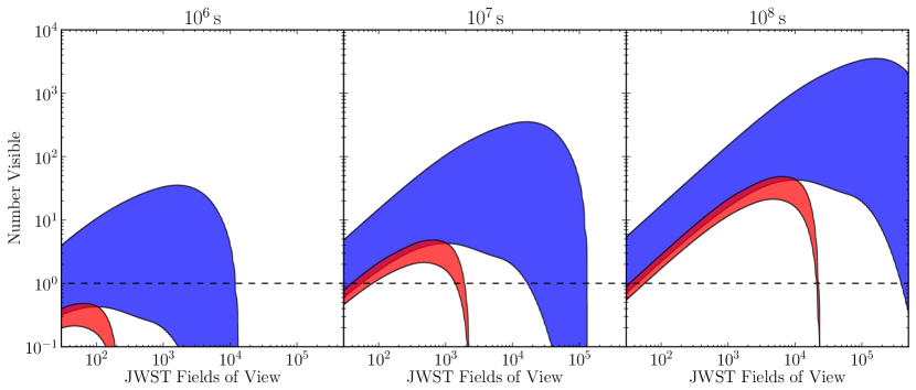
Figure 8.— The total number of PISNe observable with a campaign of $10^{6}$, $10^{7}$ and $10^{8}\,$s (from left to right) as a function of survey area for the R250 PISN model. In each case, the total campaign time is apportioned equally over the total survey area to determine the exposure time for individual pointings. The blue region represents all PISNe, the red only PISNe from $z>15$. Upper boundaries correspond to the no-feedback upper limit to the PISN rate and lower boundaries to the conservative feedback case. For reference we mark the case of only one PISN visible (dashed line).

Of particular interest in Figure 7 are the black lines representing the total number of pointings possible in $10^{6}$, $10^{7}$, and $10^{8}\,$s for a given exposure time and their location relative to the observability ranges in blue and red. $10^{6}\,$s is approximately the limit of what would be possible with a dedicated deep-field campaign; $10^{7}\,$s is the limit of the observations the JWST could make in a year assuming NIRCam is in use one third of the time; $10^{8}\,$s ($\sim$10 years) is the projected mission lifetime.

While the detection of a PISN from a ‘first’ star at very high redshifts would be exciting and is in fact possible given the detection limits of the JWST, the scarcity of sources at these redshifts means that such a detection would be highly contingent on serendipity. Even in the most optimistic case, with all available minihalos producing an R250-type PISN, the observability range for such events lies well above what is possible even in a full year of observations, though a few may be detected over the lifetime of the telescope. The detection of a PISN at lower redshifts appears to be more realistic. As the faintest PISNe (R175 and B200) are effectively unobservable, PISN searches should focus on looking for PISNe similar to the R250 and He100 models. In this case, the strategy with the highest likelihood of detection will be a mosaic survey of many moderately deep exposures. This is clear from Figure 8, where we show the number of PISNe that will be observable with the JWST in observing campaigns totalling $10^{6}$, $10^{7}$ and $10^{8}\,$s for the R250 PISN model. The exposure time for each pointing varies with the total area covered by the survey in order to keep the total observing time constant. Upper boundaries correspond to the number visible in the no-feedback case, lower boundaries to the conservative feedback case. As in Figure 7, the blue region shows the observable number from all redshifts, the red region only those from $z>15$. We see that the observable number increases until the resulting exposure time is no longer sufficient to detect PISNe. The optimal search strategy then will be to cover as large an area as possible, going only as deep as necessary, possibly in a similar manner to the ongoing Brightest of Reionizing Galaxies survey with the Hubble Space Telescope (Trenti et al., 2011; Bradley et al., 2012).

.

Included here are the observable properties of the He100 and R175 models from Kasen et al. (2011), including the observable flux and time visible (Figure 10) and the observable number for each feedback scenario (Figure 9). These plots are to be compared to Figure 5 and Figure 6 in § 3. Both cases may be detected with NIRCam beyond $z=15$ for deep exposures of $10^{6}\,$s.

Also included is an extended version of Figure 8 showing the detectable number in observing campaigns totalling $10^{6}$, $10^{7}$ and $10^{8}\,$s for all four PISN models (Figure 11). Only R250-type PISNe will be detectable above reshift 15, and R175- and B200-type PISNe will only be detectable in observing campaigns totalling greater than $10^{7}\,$s.

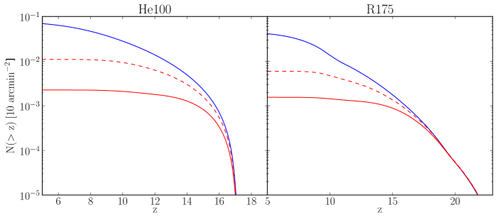
Figure 9.— Upper and lower limits for the number of PISNe per JWST FoV above redshift $z$ with different feedback prescriptions. The observable numbers for a $10^{6}\,$s exposure assuming the He100 model are shown on the left; the R175 model is employed on the right. Solid blue lines show an upper limit to the observable number in the case of no feedback, solid red lines an estimate for the observable number in our conservative feedback scenario, and dashed red lines the number in the enhanced star formation case. Note that the x-axis is scaled independently in each panel.

Figure 10.— Left: Lightcurves for the Kasen et al. (2011) He100 (top) and R175 (bottom) models as they would be observed by JWST’s F444W NIRCam filter at $z=5,10,15,20,25\>{\rm and}\>30$. The flux limits for a $10^{6}\,$s (dashed line) and $10^{4}\,$s (dotted line) exposure are shown for reference. Right: The visibility time $\Delta t_{\rm vis}$ in years for He100 (top) and R175 (bottom) as a function of redshift for each of the NIRcam wide filters. Note that the axes are scaled independently.

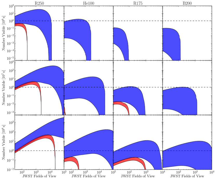
Figure 11.— The total number of PISNe observable with a campaign of $10^{6}$, $10^{7}$ and $10^{8}\,$s (from top to bottom) as a function of total survey area for a given PISN model. In each case, the total campaign time is apportioned equally over the survey area to determine the exposure time for individual pointings. The blue region represents all PISNe, the red only PISNe from $z>15$. Upper boundaries correspond to the no-feedback upper limit to the PISN rate and lower boundaries to the conservative feedback case. The dashed line marks one PISN visible. Note that not all axes are scaled the same.

References

- Abel et al. (2002) Abel, T., Bryan, G. L., & Norman, M. L. 2002, Science, 295, 93
- Alvarez et al. (2006) Alvarez, M. A., Bromm, V., & Shapiro, P. R. 2006, ApJ, 639, 621
- Alvarez et al. (2009) Alvarez, M. A., Wise, J. H., & Abel, T. 2009, ApJ, 701, L133
- Barkana & Loeb (2001) Barkana, R., & Loeb, A. 2001, Phys. Rep., 349, 125
- Barkat et al. (1967) Barkat, Z., Rakavy, G., & Sack, N. 1967, Phys. Rev. Lett., 18, 379
- Bradley et al. (2012) Bradley, L. D., et al. 2012, ApJ, submitted (arXiv:1204.3641)
- Bromm et al. (1999) Bromm, V., Coppi, P. S., & Larson, R. B. 1999, ApJ, 527, L5
- Bromm et al. (2002) —. 2002, ApJ, 564, 23
- Bromm et al. (2001) Bromm, V., Kudritzki, R. P., & Loeb, A. 2001, ApJ, 552, 464
- Bromm & Larson (2004) Bromm, V., & Larson, R. B. 2004, ARA&A, 42, 79
- Bromm & Loeb (2003) Bromm, V., & Loeb, A. 2003, Nature, 425, 812
- Bromm et al. (2003) Bromm, V., Yoshida, N., & Hernquist, L. 2003, ApJ, 596, L135
- Bromm et al. (2009) Bromm, V., Yoshida, N., Hernquist, L., & McKee, C. F. 2009, Nature, 459, 49
- Chatzopoulos & Wheeler (2012) Chatzopoulos, E., & Wheeler, J. C. 2012, ApJ, 748, 42
- Chen et al. (2011) Chen, K.-J., Heger, A., & Almgren, A. S. 2011, Comp. Phys. Communications, 182, 254
- Chiappini et al. (2011) Chiappini, C., Frischknecht, U., Meynet, G., Hirschi, R., Barbuy, B., Pignatari, M., Decressin, T., & Maeder, A. 2011, Nature, 472, 454
- Ciardi et al. (2000) Ciardi, B., Ferrara, A., & Abel, T. 2000, ApJ, 533, 594
- Clark et al. (2011) Clark, P. C., Glover, S. C. O., Smith, R. J., Greif, T. H., Klessen, R. S., & Bromm, V. 2011, Science, 331, 1040
- Couchman & Rees (1986) Couchman, H. M. P., & Rees, M. J. 1986, MNRAS, 221, 53
- Dahlén & Fransson (1999) Dahlén, T., & Fransson, C. 1999, A&A, 350, 349
- Fraley (1968) Fraley, G. S. 1968, Ap&SS, 2, 96
- Frost et al. (2009) Frost, M. I., Surace, J., Moustakas, L. A., & Krick, J. 2009, ApJ, 698, L68
- Fryer et al. (2001) Fryer, C. L., Woosley, S. E., & Heger, A. 2001, ApJ, 550, 372
- Fumagalli et al. (2011) Fumagalli, M., O’Meara, J. M., & Prochaska, J. X. 2011, Science, 334, 1245
- Furlanetto & Loeb (2003) Furlanetto, S. R., & Loeb, A. 2003, ApJ, 588, 18
- Furlanetto & Loeb (2005) —. 2005, ApJ, 634, 1
- Gal-Yam et al. (2009) Gal-Yam, A., et al. 2009, Nature, 462, 624
- Gardner et al. (2006) Gardner, J. P., et al. 2006, Space Sci. Rev., 123, 485
- Glover & Brand (2001) Glover, S. C. O., & Brand, P. W. J. L. 2001, MNRAS, 321, 385
- Greif & Bromm (2006) Greif, T. H., & Bromm, V. 2006, MNRAS, 373, 128
- Greif et al. (2012) Greif, T. H., Bromm, V., Clark, P. C., Glover, S. C. O., Smith, R. J., Klessen, R. S., Yoshida, N., & Springel, V. 2012, MNRAS, in press (arXiv:1202.5552)
- Greif et al. (2010) Greif, T. H., Glover, S. C. O., Bromm, V., & Klessen, R. S. 2010, ApJ, 716, 510
- Greif et al. (2007) Greif, T. H., Johnson, J. L., Bromm, V., & Klessen, R. S. 2007, ApJ, 670, 1
- Greif et al. (2008) Greif, T. H., Johnson, J. L., Klessen, R. S., & Bromm, V. 2008, MNRAS, 387, 1021
- Greif et al. (2011) Greif, T. H., Springel, V., White, S. D. M., Glover, S. C. O., Clark, P. C., Smith, R. J., Klessen, R. S., & Bromm, V. 2011, ApJ, 737, 75
- Haiman et al. (2000) Haiman, Z., Abel, T., & Rees, M. J. 2000, ApJ, 534, 11
- Haiman et al. (1997) Haiman, Z., Rees, M. J., & Loeb, A. 1997, ApJ, 476, 458
- Haiman et al. (1996) Haiman, Z., Thoul, A. A., & Loeb, A. 1996, ApJ, 464, 523
- Heger et al. (2003) Heger, A., Fryer, C. L., Woosley, S. E., Langer, N., & Hartmann, D. H. 2003, ApJ, 591, 288
- Heger & Woosley (2002) Heger, A., & Woosley, S. E. 2002, ApJ, 567, 532
- Hosokawa et al. (2011) Hosokawa, T., Omukai, K., Yoshida, N., & Yorke, H. W. 2011, Science, 334
- Joggerst & Whalen (2011) Joggerst, C. C., & Whalen, D. J. 2011, ApJ, 728, 129
- Johnson et al. (2007) Johnson, J. L., Greif, T. H., & Bromm, V. 2007, ApJ, 665, 85
- Karlsson et al. (2011) Karlsson, T., Bromm, V., & Bland-Hawthorn, J. 2011, Rev. Mod. Phys., submitted (arXiv:1101.4024)
- Karlsson et al. (2008) Karlsson, T., Johnson, J. L., & Bromm, V. 2008, ApJ, 679, 6
- Kasen et al. (2011) Kasen, D., Woosley, S. E., & Heger, A. 2011, ApJ, 734, 102
- Kitayama et al. (2001) Kitayama, T., Susa, H., Umemura, M., & Ikeuchi, S. 2001, MNRAS, 326, 1353
- Kitayama & Yoshida (2005) Kitayama, T., & Yoshida, N. 2005, ApJ, 630, 675
- Kitayama et al. (2004) Kitayama, T., Yoshida, N., Susa, H., & Umemura, M. 2004, ApJ, 613, 631
- Komatsu et al. (2009) Komatsu, E., et al. 2009, ApJS, 180, 330
- Kudritzki (2002) Kudritzki, R. P. 2002, ApJ, 577, 389
- Loeb (2010) Loeb, A. 2010, How Did the First Stars and Galaxies Form? (Princeton University Press)
- Machacek et al. (2001) Machacek, M. E., Bryan, G. L., & Abel, T. 2001, ApJ, 548, 509
- Mackey et al. (2003) Mackey, J., Bromm, V., & Hernquist, L. 2003, ApJ, 586, 1
- Madau et al. (1998) Madau, P., Della Valle, M., & Panagia, N. 1998, MNRAS, 297, L17
- Maio et al. (2010) Maio, U., Ciardi, B., Dolag, K., Tornatore, L., & Khochfar, S. 2010, MNRAS, 407, 1003
- Meiksin (2009) Meiksin, A. 2009, Rev. Mod. Phys., 81, 1405
- Mesinger et al. (2006a) Mesinger, A., Bryan, G. L., & Haiman, Z. 2006a, ApJ, 648, 835
- Mesinger et al. (2006b) Mesinger, A., Johnson, B. D., & Haiman, Z. 2006b, ApJ, 637, 80
- Miralda-Escudé (2003) Miralda-Escudé, J. 2003, Science, 300, 1904
- Miralda-Escudé & Rees (1997) Miralda-Escudé, J., & Rees, M. J. 1997, ApJ, 478, 57
- Mitra et al. (2011) Mitra, S., Kulkarni, G., Bagla, J. S., & Yadav, J. K. 2011, Bull. Astr. Soc. of India, 39, 563
- Mori et al. (2002) Mori, M., Ferrara, A., & Madau, P. 2002, ApJ, 571, 40
- Omukai & Nishi (1999) Omukai, K., & Nishi, R. 1999, ApJ, 518, 64
- Omukai & Yoshii (2003) Omukai, K., & Yoshii, Y. 2003, ApJ, 599, 746
- O’Shea & Norman (2007) O’Shea, B. W., & Norman, M. L. 2007, ApJ, 654, 66
- Pan et al. (2012) Pan, T., Kasen, D., & Loeb, A. 2012, MNRAS, 2809
- Pawlik et al. (2011) Pawlik, A. H., Milosavljević, M., & Bromm, V. 2011, ApJ, 731, 54
- Press & Schechter (1974) Press, W. H., & Schechter, P. 1974, ApJ, 187, 425
- Ricotti et al. (2001) Ricotti, M., Gnedin, N. Y., & Shull, J. M. 2001, ApJ, 560, 580
- Ricotti et al. (2002a) —. 2002a, ApJ, 575, 33
- Ricotti et al. (2002b) —. 2002b, ApJ, 575, 49
- Sasaki (1994) Sasaki, S. 1994, PASJ, 46, 427
- Scannapieco et al. (2005) Scannapieco, E., Madau, P., Woosley, S. E., Heger, A., & Ferrara, A. 2005, ApJ, 633, 1031
- Schaerer (2002) Schaerer, D. 2002, A&A, 382, 28
- Schaerer (2003) —. 2003, A&A, 397, 527
- Schneider et al. (2002) Schneider, R., Ferrara, A., Natarajan, P., & Omukai, K. 2002, ApJ, 571, 30
- Sedov (1959) Sedov, L. I. 1959, Similarity and Dimensional Methods in Mechanics
- Smith et al. (2007) Smith, N., et al. 2007, ApJ, 666, 1116
- Springel (2005) Springel, V. 2005, MNRAS, 364, 1105
- Springel et al. (2001) Springel, V., White, S. D. M., Tormen, G., & Kauffmann, G. 2001, MNRAS, 328, 726
- Stacy et al. (2011) Stacy, A., Bromm, V., & Loeb, A. 2011, MNRAS, 413, 543
- Stacy et al. (2010) Stacy, A., Greif, T. H., & Bromm, V. 2010, MNRAS, 403, 45
- Stacy et al. (2012) —. 2012, MNRAS, 422, 290
- Tegmark et al. (1997) Tegmark, M., Silk, J., Rees, M. J., Blanchard, A., Abel, T., & Palla, F. 1997, ApJ, 474
- Tominaga et al. (2007) Tominaga, N., Umeda, H., & Nomoto, K. 2007, ApJ, 660, 516
- Tornatore et al. (2007) Tornatore, L., Ferrara, A., & Schneider, R. 2007, MNRAS, 382, 945
- Trenti et al. (2009) Trenti, M., Stiavelli, M., & Michael Shull, J. 2009, ApJ, 700, 1672
- Trenti et al. (2011) Trenti, M., et al. 2011, ApJ, 727, L39
- Tumlinson et al. (2004) Tumlinson, J., Venkatesan, A., & Shull, J. M. 2004, ApJ, 612, 602
- Umeda & Nomoto (2003) Umeda, H., & Nomoto, K. 2003, Nature, 422, 871
- Weinmann & Lilly (2005) Weinmann, S. M., & Lilly, S. J. 2005, ApJ, 624, 526
- Whalen et al. (2004) Whalen, D., Abel, T., & Norman, M. L. 2004, ApJ, 610, 14
- Whalen et al. (2008) Whalen, D. J., van Veelen, B., O’Shea, B. W., & Norman, M. L. 2008, ApJ, 682, 49
- Wise & Abel (2005) Wise, J. H., & Abel, T. 2005, ApJ, 629, 615
- Wise & Abel (2007) —. 2007, ApJ, 665, 899
- Wise & Abel (2008) —. 2008, ApJ, 685, 40
- Wolcott-Green et al. (2011) Wolcott-Green, J., Haiman, Z., & Bryan, G. L. 2011, MNRAS, 418, 838
- Woosley et al. (2007) Woosley, S. E., Blinnikov, S., & Heger, A. 2007, Nature, 450, 390
- Yoon et al. (2012) Yoon, S.-C., Dierks, A., & Langer, N. 2012, A&A, submitted (arXiv:1201.2364)
- Yoshida et al. (2003) Yoshida, N., Abel, T., Hernquist, L., & Sugiyama, N. 2003, ApJ, 592, 645
- Yoshida et al. (2004) Yoshida, N., Bromm, V., & Hernquist, L. 2004, ApJ, 605, 579
- Yoshida et al. (2007) Yoshida, N., Oh, S. P., Kitayama, T., & Hernquist, L. 2007, ApJ, 663, 687
- Yoshida et al. (2006) Yoshida, N., Omukai, K., Hernquist, L., & Abel, T. 2006, ApJ, 652, 6