Microscopic approach to the proton asymmetry in the non–mesonic weak decay of $\Lambda$–hypernuclei

Abstract

The non–mesonic weak decay of polarized $\Lambda$–hypernuclei is studied with a microscopic diagrammatic formalism in which one– and two–nucleon induced decay mechanisms, $\vec{\Lambda}N\to NN$ and $\vec{\Lambda}NN\to NNN$, are considered together with (and on the same ground of) nucleon final state interactions. We adopt a nuclear matter formalism extended to finite nuclei via the local density approximation. Our approach adopts different one–meson–exchange weak transition potentials, while the strong interaction effects are accounted for by a Bonn nucleon–nucleon interaction. We also consider the two–pion–exchange effect in the weak transition potential. Both the two-nucleon induced decay mechanism and the final state interactions reduce the magnitude of the asymmetry. The quantum interference terms considered in the present microscopic approach give rise to an opposite behavior of the asymmetry with increasing energy cuts to that observed in models describing the nucleon final state interactions semi-classically via the intranuclear cascade code. Our results for the asymmetry parameter in ${}^{12}_{\Lambda}$C obtained with different potential models are consistent with the asymmetry measured at KEK.

I Introduction

The study of hypernuclear physics provides the main source of information on the baryon–baryon strangeness–changing weak interactions. In particular, the non–mesonic weak decay of $\Lambda$–hypernuclei has shown two challenging issues presenting some puzzling character Al02 ; Pa07 . First, we must mention the disagreement between theory and experiment for the ratio $\Gamma_{n}/\Gamma_{p}$ between the rates for the $\Lambda n\to nn$ and the $\Lambda p\to np$ non–mesonic weak decay processes. Another more recent problem concerns the asymmetry in the proton emission from the non–mesonic weak decay of polarized hypernuclei, which is our main concern in the present contribution.

A $\Lambda$–hypernucleus can be produced with some degree of polarization. Indeed, the $n(\pi^{+},K^{+})\Lambda$ reaction has been used Aj92-00 at $p_{\pi}=1.05$ GeV and small $K^{+}$ laboratory scattering angles to produce hypernuclear states with a substantial amount of spin–polarization, preferentially aligned along the line normal to the reaction plane which identifies the polarization axis. The dominant decay mechanisms for a polarized $\Lambda$–hypernucleus are the following neutron– and proton–induced processes:

$$\vec{\Lambda}n \rightarrow nn$$ (1)

$$\vec{\Lambda}p \rightarrow np.$$ (2)

It turns out that the number of protons emitted parallel to the polarization axis is different from the same quantity measured in the opposite direction. This asymmetric proton emission is a consequence of the interference between the parity–conserving and the parity–violating terms in the $\vec{\Lambda}p\to np$ weak transition potential ban90 .

Let us denote with $a^{1N}_{\Lambda}$ the intrinsic asymmetry, arising from the one–nucleon induced ($1N$) decay in Eq. (2). The one–nucleon induced decays take place within the nuclear environment and the resulting nucleon pairs can interact strongly with others nucleons of the medium before any nucleon leaves the nucleus and is detected. As a result of these final state interactions (FSI), the asymmetry measured in an experiment, $a^{\rm M}_{\Lambda}$, differs from the intrinsic value, $a^{1N}_{\Lambda}$ . Most of the theoretical models result in a negative and rather mass–independent intrinsic asymmetry. Instead, data favor a small $a^{\rm M}_{\Lambda}$, compatible with a vanishing value, for both ${}^{5}_{\Lambda}$He and ${}^{12}_{\Lambda}$C. This shows a clear disagreement between $a^{1N}_{\Lambda}$ and $a^{\rm M}_{\Lambda}$.

The reason for this disagreement can be twofold. It can be originated by the weak decay mechanism itself, which might require some improvement and the consideration of additional two–nucleon induced processes, and it may also be due to nucleon FSI. Let us start by considering the various mechanisms which contribute in the evaluation of $a^{1N}_{\Lambda}$. The theoretical models based on one–meson–exchange potentials (OME) du96 ; pa97 ; pa02 ; bar05 ; al05 ; bar07 and/or direct quark mechanisms sa02 predict $a^{1N}_{\Lambda}$ values in the range from $-0.7$ up to $-0.4$. By using an effective field theory approach, a dominating central, spin– and isospin–independent contact term was predicted in pa04 which allowed the authors to reproduce the experimental total and partial non–mesonic decay widths for ${}^{5}_{\Lambda}$He, ${}^{11}_{\Lambda}$B and ${}^{12}_{\Lambda}$C, and the asymmetry parameter for ${}^{5}_{\Lambda}$He. Motivated by this work, a scalar–isoscalar $\sigma$–meson–exchange was added to a $(\pi+K)$–exchange weak model also including a direct quark mechanism sa05 . Similarly, the $\sigma$–meson was considered together with a full OME weak potential in bar06 . Although the addition of the $\sigma$–meson may improve the calculation of $a^{1N}_{\Lambda}$, it turned out to be not enough to reproduce consistently all the decay data despite the freedom introduced by the unknown coupling constants of the $\sigma$–meson. Later, the OME weak potential was supplemented by the exchange of (uncorrelated and correlated) two–pion pairs Ch07 . The two–pion–exchange potential was obtained from a chiral unitary approach in a study of the nucleon-nucleon interaction toki and was adapted to the weak sector in ji01 for a study of the non–mesonic decay rates, while the calculation of the asymmetry was also carried out in Ch07 . The two–pion exchange mechanism turned out to introduce a significant central, spin– and isospin–independent $\Lambda N\to nN$ amplitudes and gave rise to a good reproduction of the entire set of decay rates and asymmetry data for ${}^{5}_{\Lambda}$He and ${}^{12}_{\Lambda}$C.

We now briefly comment on the effect of FSI on the asymmetry parameter. First of all, it should be noted that from a strictly quantum–mechanical point of view the only observables in non–mesonic weak decay are the total non–mesonic decay width, $\Gamma_{\rm NM}$, the spectra of the emitted nucleons and the asymmetry $a^{\rm M}_{\Lambda}$ Ba10b . It is the action of FSI which prevents the measurement of any of the non–mesonic partial decay rates and of the intrinsic asymmetry $a^{1N}_{\Lambda}$. The link between theory and experiment for both $\Gamma_{n}/\Gamma_{p}$ and $a^{1N}_{\Lambda}$, is not straightforward, since it is strongly dependent on FSI. For instance, to obtain the $\Gamma_{n}/\Gamma_{p}$ ratio from experiments, one should proceed to a deconvolution of the nucleon rescattering effects contained in the measured nucleon spectra ga03 , which requires the use of a theoretical approach for FSI. For the asymmetry parameter the situation may seem more direct, as experimental data for $a^{\rm M}_{\Lambda}$ are available. However, for a direct comparison with experiment, one must calculate the asymmetry $a^{\rm M}_{\Lambda}$, which also requires the inclusion of FSI effects. Only a couple of approaches al05 ; Ch07 calculated this observable in an appropriate way. However, both these calculations adopted an hybrid approach consisting in a shell model for describing the weak decay and a semi–classical intranuclear cascade (INC) model, for simulating FSI. The only kind of FSI effects considered within the finite nucleus approach of al05 ; Ch07 are those between the two nucleons emitted in the non–mesonic decay, which are represented by a wave function describing their relative motion under the influence of a suitable $NN$ interaction  pa02 . Although a discrepancy with data still remains for proton emission spectra ba11 ; Ba10 , one can safely assert that a formalism which takes care of FSI leads to a good agreement between theory and experiment concerning $\Gamma_{n}/\Gamma_{p}$ and $a^{\rm M}_{\Lambda}$.

In the present contribution we evaluate the asymmetry $a^{\rm M}_{\Lambda}$ employing an alternative approach to the hybrid one of al05 ; Ch07 . In our microscopic diagrammatic approach, which was developed in ba07 ; ba07b ; ba11 , both the weak decay and the nucleon FSI are part of the same quantum–mechanical problem and are thus described in a unified way. Therefore, the present formalism has a self–consistency that is not present in previous approaches. The calculation is first performed in nuclear matter and then extended to finite hypernuclei by means of a local density approximation. Clearly, our nuclear matter wave functions are less realistic than the shell model ones. However, FSI are relevant and our quantum–mechanical approach describes them more reliably than the INC. In ba11 we showed that quantum interference terms in the FSI are very important in the calculations of the observable spectra for the emitted nucleons. Moreover, in the same work we have called attention on the fact that pure (i.e., non–quantum interference terms) FSI terms and two–nucleon induced ($2N$) decay contributions originates from two different time–orderings of the same Feynman diagrams at second order in the weak transition potential.

Another contribution of the present work is the consideration for the first time of the $2N$ decays, $\vec{\Lambda}NN\to nNN$, in a calculation of the asymmetry. We will see that, although these contributions represent almost 30% of the decay width, they affect the asymmetry in a very moderate way.

The work is organized as follows. In Section II we discuss general aspects of the asymmetry in the proton emission from the decay of polarized $\Lambda$–hypernuclei. A formal derivation of the expressions needed to evaluate the asymmetry parameter is done in Section III when only $1N$ decays are included, resulting in the intrinsic asymmetry $a^{1N}_{\Lambda}$, and in Section IV when $2N$ decays and FSI are taken into account, resulting in an approximation for the observable asymmetry $a^{\rm M}_{\Lambda}$. Numerical results are presented and discussed in Section V and finally, our conclusions are given in Section VI.

II General considerations on the asymmetry parameter

Spin–polarization observables for baryon–baryon interactions are important quantities which supply additional information to the more usual total cross sections or decay rates and thus facilitate the reconstruction of the interaction amplitudes from experimental data. For nucleon–nucleon elastic scattering, a complete study of spin–polarization observables is given, for instance, in By78 . The formal derivation of the asymmetry parameter for the non–mesonic weak decay of $\Lambda$–hypernuclei is instead provided by Ra92 . Here we follow a less conventional analysis in order to remark some conceptual issues.

Let us denote with $\theta$ the angle between the momentum of the outgoing proton in the $\vec{\Lambda}p\to np$ weak process and the polarization axis of the hypernucleus. The number of emitted protons as a function of $\theta$ can be written as:

$$N_{p}(\theta)=N_{p,\,tot}(1+{\cal{A}}_{y}(\theta))/\pi\,,$$ (3)

where $N_{p,\,tot}$ is the total number of emitted protons in the decay of the polarized $\Lambda$–hypernucleus, while the function ${\cal{A}}_{y}(\theta)$ introduces an asymmetry in the distribution. By construction, it is evident that:

$$\int^{\pi}_{0}d\theta\;N_{p}(\theta)=N_{p,\,tot}\,,$$ (4)

therefore,

$$\int^{\pi}_{0}d\theta\;{\cal{A}}_{y}(\theta)=0\,.$$ (5)

Eq. (5) allows one to express ${\cal{A}}_{y}(\theta)$ as a series of odd powers of $\cos\theta$. By keeping the first term in the series expansion one has:

$${\cal{A}}_{y}(\theta)\cong C\,\cos\theta\,.$$ (6)

This expression is exact for the scattering of two elementary particles, as in the present hadronic description of the $\vec{\Lambda}p\to np$ weak decay.

It is reasonable to write the constant $C$ as the product of the polarization of the hypernucleus $P_{y}$ times a remaining constant, as follows:

$$C\equiv P_{y}\,A_{y}\,,$$ (7)

where the $A_{y}$ is the hypernuclear asymmetry parameter. Being the $\Lambda$ non–mesonic decay in a nucleus a complex process, it is evident that also the two–body induced decays $\vec{\Lambda}np\rightarrow nnp$ and $\vec{\Lambda}pp\rightarrow npp$ as well as FSI terms contribute to the observable proton number $N_{p}(\theta)$ of Eq. (3).

If we restrict to the number of protons originated from the elemntary $\vec{\Lambda}p\rightarrow np$ process, the shell model weak–coupling scheme allows us to make the following replacement:

$$P_{y}\,A_{y}\rightarrow p_{\Lambda}\,a^{1N}_{\Lambda}\,,$$ (8)

by introducing the $\Lambda$ polarization $p_{\Lambda}$ and the intrinsic $\Lambda$ asymmetry $a^{1N}_{\Lambda}$  . With these definitions, if the weak–coupling limit provides a reliable description of the hypernucleus, the intrinsic asymmetry $a^{1N}_{\Lambda}$ has the same value for any hypernuclear species.

We can thus rewrite Eq. (3) as follows:

$$N^{1N}_{p}(\theta)=N^{1N}_{p,\,tot}(1+p_{\Lambda}a^{1N}_{\Lambda}\;\cos\theta)\,,$$ (9)

where the index $1N$ refers to the fact that we are considering only the one–nucleon induced decay $\vec{\Lambda}p\to np$. From this expression, the intrinsic asymmetry is obtained as:

$$a^{1N}_{\Lambda}=\frac{1}{p_{\Lambda}}\,\frac{N^{1N}_{p}(0^{0})-N^{1N}_{p}(180^{0})}{N^{1N}_{p}(0^{0})+N^{1N}_{p}(180^{0})}\,.$$ (10)

Once we consider the two–body induced decay process and FSI as well, the number of emitted protons takes the following form:

$$N_{p}(\theta)\equiv N^{1N}_{p}(\theta)+N^{2N+FSI}_{p}(\theta)\,.$$ (11)

As long as $N^{2N+FSI}_{p}(\theta)$ has a linear dependence on $\cos\theta$, it is possible to define an observable asymmetry parameter, $a_{\Lambda}^{1N+2N+FSI}$, given by a relation which is analogous to the one in Eq. (10), which can be compared with the experimental data for the asymmetry $a_{\Lambda}^{\rm M}$.

III Formal derivation of the intrinsic asymmetry

For computational purposes, we may assume that the hypernucleus is completely polarized. The intrinsic asymmetry is then given by Eq.(10) with $p_{\Lambda}=P_{y}=1$.

We now focus on the evaluation of the $N^{1N}_{p}(\theta)$ spectrum. For our practical purpose, we can suppose that the polarized $\Lambda$ has its spin aligned with the polarization axis (which thus coincides with the quantization axis). The evaluation of $N^{1N}_{p}(\theta)$ is rather similar to the evaluation of the proton kinetic energy spectrum $N_{p}(T_{p})$ described in ba07 ; ba07b ; ba11 , except for two points: $i)$ the angle $\theta$ replaces the proton kinetic energy $T_{p}$ as variable and $ii)$ we no longer sum over the two spin projections of the $\Lambda$, but retain only the up component. This second point requires a new evaluation of the spin–summation. To build up an analytical expression for $N^{1N}_{p}(\theta)$, let us first express it in terms of the more familiar decay widths as follows:

$$N^{1N}_{p}(\theta)=\bar{\Gamma}_{p}(\theta)\,,$$ (12)

with $\bar{\Gamma}_{p}(\theta)\equiv\Gamma_{p}(\theta)/\Gamma_{\rm NM}$, where $\Gamma_{\rm NM}$ is the total non–mesonic weak decay rate and $\Gamma_{p}(\theta)$ is the proton induced decay rate as a function of $\theta$ . With these definitions, the $N^{1N}_{p}(\theta)$ spectrum is normalized per non–mesonic weak decay.

Before we give explicit expressions for the $\theta$–dependent proton spectrum, it is convenient to introduce first the weak transition potential:

$$V^{\Lambda N\to NN}(q)=\sum_{\tau=0,1}{\cal O}_{\tau}{\cal V}_{\tau}^{\Lambda N\to NN}(q)~{},$$ (13)

where the isospin dependence is given by

$${\cal O}_{\tau}=\left\{\begin{array}[]{c}~{}1~{}~{}~{}~{}~{}\mbox{for}~{}~{}\tau=0\\ \mbox{\boldmath$\tau$}_{1}\cdot\mbox{\boldmath$\tau$}_{2}~{}\mbox{for}~{}~{}\tau=1~{}.\end{array}\right.$$ (16)

The values $0$ and $1$ for $\tau$ refer to the isoscalar and isovector parts of the interactions, respectively. The spin and momentum dependence of the weak transition potential is given by the function:

$${\cal V}_{\tau}^{\Lambda N\to NN}(q) = (G_{F}m_{\pi}^{2})\;\{S_{\tau}(q)\;\mbox{\boldmath$\sigma$}_{1}\cdot\mbox{\boldmath$\hat{q}$}+S^{\prime}_{\tau}(q)\;\mbox{\boldmath$\sigma$}_{2}\cdot\mbox{\boldmath$\hat{q}$}+P_{C,\tau}(q)$$

$$+P_{L,\tau}(q)\mbox{\boldmath$\sigma$}_{1}\cdot\mbox{\boldmath$\hat{q}$}\;\mbox{\boldmath$\sigma$}_{2}\cdot\mbox{\boldmath$\hat{q}$}+P_{T,\tau}(q)(\mbox{\boldmath$\sigma$}_{1}\times\mbox{\boldmath$\hat{q}$})\cdot(\mbox{\boldmath$\sigma$}_{2}\times\mbox{\boldmath$\hat{q}$})$$

$$+iS_{V,\tau}(q)\mbox{\boldmath$(\sigma$}_{1}\times\mbox{\boldmath$\sigma$}_{2})\cdot\mbox{\boldmath$\hat{q}$}\}~{},$$

where the index 1 (2) refers to the strong (weak) vertex. The functions $S_{\tau}(q)$, $S^{\prime}_{\tau}(q)$, $P_{C,\tau}(q)$, $P_{L,\tau}(q)$, $P_{T,\tau}(q)$ and $S_{V,\tau}(q)$, which include short range correlations, can be adjusted to reproduce any weak transition potential. Explicit expressions can be found in ba03 . The $S^{\prime}s$ ($P^{\prime}s$) functions are the parity–violating (parity–conserving) contributions of the weak transition potential.

In Fig. 1 we show the Goldstone diagram which has to be evaluated in the calculation of $N^{1N}_{p}(\theta)$.

Figure 1: Direct Goldstone diagram corresponding to the square of the $\vec{\Lambda}p\rightarrow np$ decay amplitude.

The spin summation for this diagram is performed for all particles except for the $\Lambda$, which is assumed to have spin up. This summation reads:

$${\cal S}^{dir,\,\uparrow}_{\tau\tau^{\prime}}(q) = 2\;\{S_{\tau}(q)S_{\tau^{\prime}}(q)+S^{\prime}_{\tau}(q)S^{\prime}_{\tau^{\prime}}(q)+P_{L,\tau}(q)P_{L,\tau^{\prime}}(q)+P_{C,\tau}(q)P_{C,\tau^{\prime}}(q)$$

$$+2\,P_{T,\tau}(q)P_{T,\tau^{\prime}}(q)+2\,S_{V,\tau}(q)S_{V,\tau^{\prime}}(q)$$

$$-2\,[S_{\tau}(q)P_{C,\tau^{\prime}}(q)+S_{\tau^{\prime}}(q)P_{C,\tau}(q)+S^{\prime}_{\tau}(q)P_{L,\tau^{\prime}}(q)+S^{\prime}_{\tau^{\prime}}(q)P_{L,\tau}(q)$$

$$+2\,S_{V,\tau}(q)P_{T,\tau^{\prime}}(q)+2\,S_{V,\tau^{\prime}}(q)P_{T,\tau}(q)]\,\hat{q_{z}}\}\,.$$

It is instructive to note that in the summation over the $\Lambda$ spin projection,

$${\cal S}^{dir,\,\uparrow}_{\tau\tau^{\prime}}(q)+{\cal S}^{dir,\,\downarrow}_{\tau\tau^{\prime}}(q) = 4\;\{S_{\tau}(q)S_{\tau^{\prime}}(q)+S^{\prime}_{\tau}(q)S^{\prime}_{\tau^{\prime}}(q)+P_{L,\tau}(q)P_{L,\tau^{\prime}}(q)+P_{C,\tau}(q)P_{C,\tau^{\prime}}(q)$$ (19)

$$+2\,P_{T,\tau}(q)P_{T,\tau^{\prime}}(q)+2\,S_{V,\tau}(q)S_{V,\tau^{\prime}}(q)\}\,,$$

the terms between square brackets in Eq. (III) are no longer present. These terms are responsible for the asymmetry parameter and are clearly due to interferences between parity–violating and parity–conserving contributions of the weak transition potential in Eq. (III).

Following ba07 ; ba07b , we introduce now a partial, isospin–dependent decay width, $\Gamma^{(i)}_{\tau\,\tau^{\prime}}(\mbox{\boldmath$k$},k_{F},\theta)$, where $k$ is the momentum of the $\Lambda$ and $k_{F}$ the Fermi momentum of nuclear matter. This is done for the two isospin channels, $\tau$, $\tau^{\prime}=0,1$, contributing to the spectra. In Fig. 2 we depict the charge–exchange and charge–conserving contributions. The distinction between the two terms is important in the evaluation of $N^{1N}_{p}(\theta)$ as the kinematics of the proton attached to the weak vertex is different from the one outgoing from the strong vertex.

Figure 2: The two isospin contributions to the direct Goldstone diagram for the $\vec{\Lambda}p\to np$ decay. $(a)$ is the charge–exchange contribution, which is not vanishing only for $\tau=\tau^{\prime}=1$, while $(b)$ is the charge–conserving one. The double arrows represent the $\Lambda$ and carry a momentum $k$, while dashed lines represent the weak transition potential with momentum $q$. The momentum assigned to each intermediate nucleon line is: $\mbox{\boldmath$k$}-\mbox{\boldmath$q$}$ for the left-most nucleon line ($p$ in (a) or $n$ in (b)), $h$ for $p^{-1}$ and $\mbox{\boldmath$h$}+\mbox{\boldmath$q$}$ for the right-most nucleon line ($n$ in (a) or $p$ in (b)).

The partial, isospin–dependent decay widths for the two terms of Fig. 2 are:

$$\Gamma^{(a)}_{1,1}(\mbox{\boldmath$k$},k_{F},\theta) = (G_{F}m_{\pi}^{2})^{2}\frac{1}{(2\pi)^{5}}\int\int d\mbox{\boldmath$q$}d\mbox{\boldmath$h$}\;{\cal S}^{dir,\,\uparrow}_{11}(q)\;\theta(q_{0})\theta(|\mbox{\boldmath$k-q$}|-k_{F})$$

$$\times\theta(|\mbox{\boldmath$h$}+\mbox{\boldmath$q$}|-k_{F})\theta(k_{F}-|\mbox{\boldmath$h$}|)\;\delta(q_{0}-(E_{N}(\mbox{\boldmath$h$}+\mbox{\boldmath$q$})-E_{N}(\mbox{\boldmath$h$})))$$

$$\times\delta(\cos\theta-(\mbox{\boldmath$k-q$})_{z}/|\mbox{\boldmath$k-q$}|)\,,$$

and

$$\Gamma^{(b)}_{\tau\,\tau^{\prime}}(\mbox{\boldmath$k$},k_{F},\theta) = (G_{F}m_{\pi}^{2})^{2}\frac{1}{(2\pi)^{5}}\int\int d\mbox{\boldmath$q$}d\mbox{\boldmath$h$}\;{\cal S}^{dir,\,\uparrow}_{\tau\tau^{\prime}}(q)\;\theta(q_{0})\theta(|\mbox{\boldmath$k-q$}|-k_{F})$$

$$\times\theta(|\mbox{\boldmath$h$}+\mbox{\boldmath$q$}|-k_{F})\theta(k_{F}-|\mbox{\boldmath$h$}|)\;\delta(q_{0}-(E_{N}(\mbox{\boldmath$h$}+\mbox{\boldmath$q$})-E_{N}(\mbox{\boldmath$h$})))$$

$$\times\delta(\cos\theta-(\mbox{\boldmath$h+q$})_{z}/|\mbox{\boldmath$h+q$}|)\,,$$

where the kinematics is explained in Fig. 2. Label $(a)$ refers to the charge–exchange contribution (proton attached to the $\Lambda$ vertex) and label $(b)$ represents the charge–conserving term (proton attached in the strong vertex). In previous equations one has $q_{0}=k_{0}-E_{N}(\mbox{\boldmath$k-q$})-V_{N}$, $k_{0}$ being the total energy of the $\Lambda$, $E_{N}$ the nucleon total free energy and $V_{N}$ the nucleon binding energy. After performing the isospin summation we obtain:

$$\Gamma_{p}=4\Gamma^{(a)}_{1,1}+\Gamma^{(b)}_{1,1}+\Gamma^{(b)}_{0,0}-\Gamma^{(b)}_{0,1}-\Gamma^{(b)}_{1,0}\,,$$ (22)

where the $(\mbox{\boldmath$k$},k_{F},\theta)$–dependence of all functions is omitted for simplicity. Finally, the decay rates for a finite hypernucleus are obtained by the local density approximation, i.e., after averaging the above partial width over the $\Lambda$ momentum distribution in the considered hypernucleus, $|\widetilde{\psi}_{\Lambda}(\mbox{\boldmath$k$})|^{2}$, and over the local Fermi momentum, $k_{F}(r)=\{3\pi^{2}\rho(r)/2\}^{1/3}$, $\rho(r)$ being the density profile of the nuclear core. One thus has:

$$\Gamma_{p}(\theta)=\int d\mbox{\boldmath$k$}\,|\widetilde{\psi}_{\Lambda}(\mbox{\boldmath$k$})|^{2}\int d\mbox{\boldmath$r$}\,|\psi_{\Lambda}(\mbox{\boldmath$r$})|^{2}\Gamma_{p}(\mbox{\boldmath$k$},k_{F}(r),\theta)~{},$$ (23)

where $\psi_{\Lambda}(\mbox{\boldmath$r$})$ is the Fourier transform of $\widetilde{\psi}_{\Lambda}(\mbox{\boldmath$k$})$. The $\Lambda$ total energy is given by $k_{0}=m_{\Lambda}+\mbox{\boldmath$k$}^{2}/(2m_{\Lambda})+V_{\Lambda}$, where $V_{\Lambda}$ is a binding potential.

Finally, by inserting the quantities $N^{1N}_{p}(\theta)=\bar{\Gamma}_{p}(\theta)=\Gamma_{p}(\theta)/\Gamma_{\rm NM}$ for $0^{0}$ and $180^{0}$ in Eq. (10) with $p_{\Lambda}=1$, the intrinsic asymmetry $a^{1N}_{\Lambda}$ is obtained.

IV Effect of the strong interaction on the asymmetry

The evaluation of the asymmetry $a^{1N+2N+FSI}_{\Lambda}$, which includes the effects of both $2N$ and FSI–induced decay processes, is an involved task and, up to now, analytical expressions were given only for the intrinsic asymmetry $a^{1N}_{\Lambda}$, while numerical calculations were performed for $a^{1N+FSI}_{\Lambda}$ by using the aforementioned hybrid approach incorporating the INC al05 ; Ch07 . In this section we present for the first time analytical expressions for $a^{1N+2N+FSI}_{\Lambda}$.

We follow similar steps as in the last section in order to derive $N^{2N+FSI}_{p}(\theta)$, which provides the total proton spectrum $N^{1N+2N+FSI}_{p}(\theta)=N^{1N}_{p}(\theta)+N^{2N+FSI}_{p}(\theta)$. This is done by introducing the set of Feynman diagrams depicted in Fig. 3 to take care of $2N$ decays and FSI effects which result from the action of the nucleon–nucleon strong interaction involving the nucleons produced by the weak decay and nucleons of the medium. The choice of the set

Figure 3: The set of Feynman diagrams considered in this work for the in–medium $\Lambda$ self–energy. The different time–ordering terms of these diagrams contribute to $2N$ and FSI–induced decays.

of diagrams in Fig. 3 is motivated by previous calculations ba07 ; ba07b ; ba11 , which show that these are the dominant contributions in the evaluation of the nucleon emission spectra. Each Feynman diagram is the sum of a number of time–ordering (i.e, Goldstone) diagrams. It is in terms of these Goldstone diagrams that one can differentiate among $1N$, $2N$, pure FSI and quantum interference terms (QIT) between $1N$ or $2N$ and FSI contributions. This point is relevant as it shows that, from a quantum–mechanical perspective, each of the above processes are included in a unitary description. More details on this point are given in ba11 .

Since in the evaluation with Goldstone diagrams the $2N$ decays are separated contributions from FSI–induced decays (which are divided in pure FSI and QIT terms), the $2N+FSI$ proton spectrum reads:

$$N^{2N+FSI}_{p}(\theta)=N^{2N}_{p}(\theta)+N^{FSI}_{p}(\theta)\,,$$ (24)

where:

$$N^{2N}_{p}(\theta) = \bar{\Gamma}_{np}(\theta)+2\bar{\Gamma}_{pp}(\theta)~{},$$ (25)

$$N^{FSI}_{p}(\theta) = \sum_{i,\,f}N_{f}\,\bar{\Gamma}_{i,f}(\theta)~{}.$$ (26)

Here, $\bar{\Gamma}\equiv\Gamma/\Gamma_{\rm NM}$ stands for the decay rate of a particular decay mode normalized per non-mesonic weak decay. The functions $\bar{\Gamma}_{np}$ and $\bar{\Gamma}_{pp}$ represent the $\vec{\Lambda}np\to nnp$ and $\vec{\Lambda}pp\to npp$ decay processes, respectively, while $\bar{\Gamma}_{i,f}$ represent either pure FSI Goldstone diagrams or QIT Goldstone diagrams, accounting for the quantum interference among $1N$ or $2N$ and FSI–induced decay processes. The index $i$ in $\bar{\Gamma}_{i,f}$ is used to label a particular Goldstone diagram obtained from the Feynman diagrams in Fig. 3, while $f$ denotes the final physical states of the Goldstone diagram and in the present case can take the values $f=np$ (cut on $2p1h$ states) and $f=npN$ (cut on $3p2h$ states), with $N=n$, $p$, since we need at least one proton in the final state to obtain $N^{1N+2N+FSI}_{p}(\theta)$. Finally, $N_{f}$ is the number of protons contained in the multinucleon state $f$.

At this point it is necessary to introduce the adopted nucleon–nucleon strong potential:

$$V^{NN}(t)=\sum_{\tau_{N}=0,1}{\cal O}_{\tau_{N}}{\cal V}_{\tau_{N}}^{NN}(t)~{},$$ (27)

where $t$ is the momentum carried by the strong interaction, ${\cal O}_{\tau_{N}}$ is defined in Eq. (16) and the spin and momentum dependence of the interaction is given by:

$${\cal V}_{\tau_{N}}^{NN}(t) = \frac{f_{\pi}^{2}}{m_{\pi}^{2}}\;\{{\cal V}_{C,\,\tau_{N}}(t)+{\cal V}_{L,\,\tau_{N}}(t)\mbox{\boldmath$\sigma$}_{1}\cdot\mbox{\boldmath$\hat{t}$}\;\mbox{\boldmath$\sigma$}_{2}\cdot\mbox{\boldmath$\hat{t}$}$$

$$+{\cal V}_{T,\,\tau_{N}}(t)(\mbox{\boldmath$\sigma$}_{1}\times\mbox{\boldmath$\hat{t}$})\cdot(\mbox{\boldmath$\sigma$}_{2}\times\mbox{\boldmath$\hat{t}$})\}~{},$$

where the functions ${\cal V}_{C,\,\tau_{N}}(t)$, ${\cal V}_{L,\,\tau_{N}}(t)$ and ${\cal V}_{T,\,\tau_{N}}(t)$ are adjusted to reproduce any strong interaction.

In the calculation of the diagrams in Fig. 3 the isospin summation is particularly complex as one has to differentiate the isospin projection of each particle. We give details on this aspect in the present Section and in the Appendix. The main features of the momentum dependence of the diagrams were discussed in ba11 and references therein. However, the important point in the evaluation of the asymmetry is the spin dependence of the diagrams.

We thus start by considering the spin summation for each Goldstone diagram obtained from Fig. 3. This sum is performed for all particles except the $\Lambda$, which again is assumed to have spin up with respect to the polarization axis. For the diagrams $pp$ and $hh$ we obtain:

$${\cal S}^{pp\,(hh)}_{\tau\tau^{\prime};\tau_{N}{\tau^{\prime}}_{N}}(q,t)=2\;{\cal S}^{dir,\,\uparrow}_{\tau\tau^{\prime}}(q)\;\{{\cal V}_{C,\,\tau_{N}}(t){\cal V}_{C,\,\tau^{\prime}_{N}}(t)+{\cal V}_{L,\,\tau_{N}}(t){\cal V}_{L,\,\tau^{\prime}_{N}}(t)+2\,{\cal V}_{T,\,\tau_{N}}(t){\cal V}_{T,\,\tau^{\prime}_{N}}(t)\}\,,$$ (29)

where ${\cal S}^{dir,\,\uparrow}_{\tau\tau^{\prime}}(q)$ is given in Eq. (III). The spin summation is more complex for the $ph$ diagram. It is convenient to split it in the sum of two terms:

$${\cal S}^{ph}_{\tau\tau^{\prime};\tau_{N}{\tau^{\prime}}_{N}}(q,t)\equiv{\cal S}^{ph,\,\rm no-asym}_{\tau\tau^{\prime};\tau_{N}{\tau^{\prime}}_{N}}(q,t)+{\cal S}^{ph,\,\rm asym}_{\tau\tau^{\prime};\tau_{N}{\tau^{\prime}}_{N}}(q,t)\,,$$ (30)

where

$${\cal S}^{ph,\,\rm no-asym}_{\tau\tau^{\prime};\tau_{N}{\tau^{\prime}}_{N}}(q,t) = 4\;\{(S_{\tau}(q)S_{\tau^{\prime}}(q)+P_{C,\tau}(q)P_{C,\tau^{\prime}}(q))\;{\cal W}^{C}_{\tau_{N}{\tau^{\prime}}_{N}}(t)$$

$$\;+(S^{\prime}_{\tau}(q)S^{\prime}_{\tau^{\prime}}(q)+P_{L,\tau}(q)P_{L,\tau^{\prime}}(q))\;{\cal W}^{L}_{\tau_{N}{\tau^{\prime}}_{N}}(t)$$

$$\;+2(\,S_{V,\tau}(q)S_{V,\tau^{\prime}}(q)+P_{T,\tau}(q)P_{T,\tau^{\prime}}(q))\;{\cal W}^{C}_{\tau_{N}{\tau^{\prime}}_{N}}(t)\}\,,$$

represents the term which does not contribute to the asymmetry and

$${\cal S}^{ph,\,\rm asym}_{\tau\tau^{\prime};\tau_{N}{\tau^{\prime}}_{N}}(q,t) = -8\;\{(S_{\tau}(q)P_{C,\tau^{\prime}}(q)+S_{\tau^{\prime}}(q)P_{C,\tau}(q))\;{\cal W}^{C}_{\tau_{N}{\tau^{\prime}}_{N}}(t)$$

$$\;+(S^{\prime}_{\tau}(q)P_{L,\tau^{\prime}}(q)+S^{\prime}_{\tau^{\prime}}(q)P_{L,\tau}(q))\;{\cal W}^{L}_{\tau_{N}{\tau^{\prime}}_{N}}(t)$$

$$\;+2(\,S_{V,\tau}(q)P_{T,\tau^{\prime}}(q)+S_{V,\tau^{\prime}}(q)P_{T,\tau}(q))\;{\cal W}^{C}_{\tau_{N}{\tau^{\prime}}_{N}}(t)\}\,\hat{q_{z}}\,,$$

is the term responsible for the asymmetry. In these expressions we have introduced the functions:

$${\cal W}^{C}_{\tau_{N}{\tau^{\prime}}_{N}} = {\cal V}_{C,\,\tau_{N}}{\cal V}_{C,\,\tau^{\prime}_{N}}+{\cal V}_{L,\,\tau_{N}}{\cal V}_{L,\,\tau^{\prime}_{N}}+2\,{\cal V}_{T,\,\tau_{N}}{\cal V}_{T,\,\tau^{\prime}_{N}}\,,$$ (33)

$${\cal W}^{L}_{\tau_{N}{\tau^{\prime}}_{N}} = {\cal V}_{C,\,\tau_{N}}{\cal V}_{C,\,\tau^{\prime}_{N}}-{\cal V}_{T,\,\tau_{N}}{\cal V}_{T,\,\tau^{\prime}_{N}}+(-1+2\hat{q}\cdot\hat{t})\,({\cal V}_{L,\,\tau_{N}}{\cal V}_{L,\,\tau^{\prime}_{N}}-{\cal V}_{T,\,\tau_{N}}{\cal V}_{T,\,\tau^{\prime}_{N}})\,,$$

$${\cal W}^{T}_{\tau_{N}{\tau^{\prime}}_{N}} = {\cal V}_{C,\,\tau_{N}}{\cal V}_{C,\,\tau^{\prime}_{N}}+{\cal V}_{T,\,\tau_{N}}{\cal V}_{T,\,\tau^{\prime}_{N}}+\hat{q}\cdot\hat{t}\,({\cal V}_{L,\,\tau_{N}}{\cal V}_{L,\,\tau^{\prime}_{N}}-{\cal V}_{T,\,\tau_{N}}{\cal V}_{T,\,\tau^{\prime}_{N}})\,,$$

representing the effect of the strong interaction. For simplicity, the $t$–dependence in both the ${\cal W}$’s and ${\cal V}$’s has been omitted in these expressions. Although Eq. (IV) is a more complicated expression than the ones in Eqs. (III) and (29), again the asymmetry is originated from the interference between parity–violating ($S$’s) and parity–conserving ($P$’s) terms of the weak transition potential.

The next step is to implement the momentum and isospin summation for each Goldstone diagram. In this Section we choose the Goldstone diagram in Fig. 4 as a representative example for this evaluation and we leave to the Appendix the remaining contributions. This diagram is a particular time–ordering contribution stemming from the $hh$ Feynman diagram in Fig. 3. It contributes to the two–nucleon induced decay mechanisms $\vec{\Lambda}np\rightarrow nnp$ and $\vec{\Lambda}pp\rightarrow npp$ with one and two protons in the final states, respectively.

Figure 4: Time–ordering term from Feynman diagram $hh$ in Fig. 3 contributing to $2N$ decays. The momentum carried by the weak transition potential (strong interaction) is $q$ ($t$). The momentum of each particle is $k$ for $p_{\Lambda}$, $\mbox{\boldmath$k$}-\mbox{\boldmath$q$}$ for $p_{1}$, $\mbox{\boldmath$k$}-\mbox{\boldmath$t$}+\mbox{\boldmath$q$}$ for $p_{2}$, $\mbox{\boldmath$h$}+\mbox{\boldmath$t$}$ for $p^{\prime}_{2}$, $h$ for $h_{2}$, $\mbox{\boldmath$h^{\prime}$}+\mbox{\boldmath$t$}$ for $p_{3}$ and $h^{\prime}$ for $h_{3}$.

Protons in the final state can be in any of the nucleon lines labelled by $p_{1}$, $p_{2}$ and $p_{3}$ in Fig. 4. To deal with this matter, it is again convenient to introduce some partial, isospin dependent decay widths. For the $\vec{\Lambda}np\rightarrow nnp$ Goldstone diagram of Fig. 4 we define the following rates:

$$\Gamma^{hh,\,p_{1}}_{\tau\tau^{\prime};\tau_{N}{\tau^{\prime}}_{N}}(\mbox{\boldmath$k$},k_{F},\theta) = \frac{(G_{F}m_{\pi}^{2})^{2}}{(2\pi)^{5}}\left(\frac{f_{\pi}^{2}}{4\pi}\right)^{2}\frac{1}{m_{\pi}^{4}}\frac{2}{(2\pi)^{2}}\;\int d\mbox{\boldmath$q$}\int d\mbox{\boldmath$t$}\int d\mbox{\boldmath$h$}\int d\mbox{\boldmath$h^{\prime}$}\,\theta(q_{0})$$

$$\times\theta(|\mbox{\boldmath$k$}-\mbox{\boldmath$q$}|-k_{F})\theta(|\mbox{\boldmath$h$}-\mbox{\boldmath$t$}|-k_{F})\,\theta(|\mbox{\boldmath$h$}-\mbox{\boldmath$t$}+\mbox{\boldmath$q$}|-k_{F})\theta(k_{F}-|\mbox{\boldmath$h$}|)$$

$$\times\theta(|\mbox{\boldmath$h^{\prime}$}+\mbox{\boldmath$t$}|-k_{F})\,\theta(k_{F}-|\mbox{\boldmath$h^{\prime}$}|)\;\delta(\cos\theta-(\mbox{\boldmath$k-q$})_{z}/|\mbox{\boldmath$k-q$}|)$$

$$\times\delta(q_{0}-(E_{N}(\mbox{\boldmath$h$}-\mbox{\boldmath$t$}+\mbox{\boldmath$q$})-E_{N}(\mbox{\boldmath$h$})+E_{N}(\mbox{\boldmath$h^{\prime}$}+\mbox{\boldmath$t$})-E_{N}(\mbox{\boldmath$h^{\prime}$}))$$

$$\times\frac{{\cal S}^{hh}_{\tau\tau^{\prime};\tau_{N}{\tau^{\prime}}_{N}}(q,t)}{(E_{N}(\mbox{\boldmath$h$}-\mbox{\boldmath$t$})-E_{N}(\mbox{\boldmath$h$})+E_{N}(\mbox{\boldmath$h^{\prime}$}+\mbox{\boldmath$t$})-E_{N}(\mbox{\boldmath$h^{\prime}$}))^{2}}\,,$$

$$\Gamma^{hh,\,p_{2}}_{\tau\tau^{\prime};\tau_{N}{\tau^{\prime}}_{N}}(\mbox{\boldmath$k$},k_{F},\theta) = \Gamma^{hh,\,p_{1}}_{\tau\tau^{\prime};\tau_{N}{\tau^{\prime}}_{N}}(\mbox{\boldmath$k$},k_{F},\theta)|$$

$$\delta(\cos\theta-(\mbox{\boldmath$k-q$})_{z}/|\mbox{\boldmath$k-q$}|)\rightarrow\delta(\cos\theta-(\mbox{\boldmath$h-t+q$})_{z}/|\mbox{\boldmath$h-t+q$}|)\,,$$

$$\Gamma^{hh,\,p_{3}}_{\tau\tau^{\prime};\tau_{N}{\tau^{\prime}}_{N}}(\mbox{\boldmath$k$},k_{F},\theta) = \Gamma^{hh,\,p_{1}}_{\tau\tau^{\prime};\tau_{N}{\tau^{\prime}}_{N}}(\mbox{\boldmath$k$},k_{F},\theta)|$$

$$\delta(\cos\theta-(\mbox{\boldmath$k-q$})_{z}/|\mbox{\boldmath$k-q$}|)\rightarrow\delta(\cos\theta-(\mbox{\boldmath$h^{\prime}+t$})_{z}/|\mbox{\boldmath$h^{\prime}+t$}|)\,,$$

each one for the final proton occupying the nucleon line $p_{1}$, $p_{2}$ or $p_{3}$ in the diagram, respectively. In a similar way, for the reaction $\vec{\Lambda}pp\rightarrow npp$, we have:

$$\Gamma^{hh,\,p_{1},\,p_{3}}_{\tau\tau^{\prime};\tau_{N}{\tau^{\prime}}_{N}}(\mbox{\boldmath$k$},k_{F},\theta) = \frac{(G_{F}m_{\pi}^{2})^{2}}{(2\pi)^{5}}\left(\frac{f_{\pi}^{2}}{4\pi}\right)^{2}\frac{1}{m_{\pi}^{4}}\frac{2}{(2\pi)^{2}}\;\int d\mbox{\boldmath$q$}\int d\mbox{\boldmath$t$}\int d\mbox{\boldmath$h$}\int d\mbox{\boldmath$h^{\prime}$}\,\theta(q_{0})$$

$$\times\theta(|\mbox{\boldmath$k$}-\mbox{\boldmath$q$}|-k_{F})\theta(|\mbox{\boldmath$h$}-\mbox{\boldmath$t$}|-k_{F})\,\theta(|\mbox{\boldmath$h$}-\mbox{\boldmath$t$}+\mbox{\boldmath$q$}|-k_{F})\theta(k_{F}-|\mbox{\boldmath$h$}|)$$

$$\times\theta(|\mbox{\boldmath$h^{\prime}$}+\mbox{\boldmath$t$}|-k_{F})\,\theta(k_{F}-|\mbox{\boldmath$h^{\prime}$}|)$$

$$\times(\delta(\cos\theta-(\mbox{\boldmath$k-q$})_{z}/|\mbox{\boldmath$k-q$}|)+\delta(\cos\theta-(\mbox{\boldmath$h^{\prime}+t$})_{z}/|\mbox{\boldmath$h^{\prime}+t$}|))/2$$

$$\times\delta(q_{0}-(E_{N}(\mbox{\boldmath$h$}-\mbox{\boldmath$t$}+\mbox{\boldmath$q$})-E_{N}(\mbox{\boldmath$h$})+E_{N}(\mbox{\boldmath$h^{\prime}$}+\mbox{\boldmath$t$})-E_{N}(\mbox{\boldmath$h^{\prime}$}))$$

$$\times\frac{{\cal S}^{hh}_{\tau\tau^{\prime};\tau_{N}{\tau^{\prime}}_{N}}(q,t)}{(E_{N}(\mbox{\boldmath$h$}-\mbox{\boldmath$t$})-E_{N}(\mbox{\boldmath$h$})+E_{N}(\mbox{\boldmath$h^{\prime}$}+\mbox{\boldmath$t$})-E_{N}(\mbox{\boldmath$h^{\prime}$}))^{2}}\,,$$

$$\Gamma^{hh,\,p_{2},\,p_{3}}_{\tau\tau^{\prime};\tau_{N}{\tau^{\prime}}_{N}}(\mbox{\boldmath$k$},k_{F},\theta) = \Gamma^{hh,\,p_{1},\,p_{3}}_{\tau\tau^{\prime};\tau_{N}{\tau^{\prime}}_{N}}(\mbox{\boldmath$k$},k_{F},\theta)|$$

$$\delta(\cos\theta-(\mbox{\boldmath$k-q$})_{z}/|\mbox{\boldmath$k-q$}|)\rightarrow\delta(\cos\theta-(\mbox{\boldmath$h-t+q$})_{z}/|\mbox{\boldmath$h-t+q$}|)\,,$$

where the sum of the two delta functions in $\cos\theta$ in Eq.(IV) is divided by two in order to retain this multiplicative factor in front of $\bar{\Gamma}_{pp}(\theta)$ in Eq. (25). Note that charge conservation does not allow particles $p_{1}$ and $p_{2}$ to be two protons simultaneously.

The next step is to implement the isospin summation. For the $\vec{\Lambda}np\rightarrow nnp$ decay we obtain:

$$\Gamma^{hh,\,p_{1}}_{np} = 4(5{\Gamma}^{hh,\,p_{1}}_{11,11}+{\Gamma}^{hh,\,p_{1}}_{00,00}-2{\Gamma}^{hh,\,p_{1}}_{11,00})\,,$$ (39)

$$\Gamma^{hh,\,p_{2}}_{np} = 5{\Gamma}^{hh,\,p_{2}}_{11,11}+{\Gamma}^{hh,\,p_{2}}_{00,00}-10{\Gamma}^{hh,\,p_{2}}_{01,11}+5{\Gamma}^{hh,\,p_{2}}_{00,11}$$

$$+{\Gamma}^{hh,\,p_{2}}_{11,00}-2{\Gamma}^{hh,\,p_{2}}_{01,00}-2{\Gamma}^{hh,\,p_{2}}_{11,01}-2{\Gamma}^{hh,\,p_{2}}_{11,01}$$

$$-2{\Gamma}^{hh,\,p_{2}}_{00,01}+4{\Gamma}^{hh,\,p_{2}}_{01,01}\,,$$

$$\Gamma^{hh,\,p_{3}}_{np} = 5{\Gamma}^{hh,\,p_{3}}_{11,11}+{\Gamma}^{hh,\,p_{3}}_{00,00}+10{\Gamma}^{hh,\,p_{3}}_{01,11}+5{\Gamma}^{hh,\,p_{3}}_{00,11}$$

$$+{\Gamma}^{hh,\,p_{3}}_{11,00}+2{\Gamma}^{hh,\,p_{3}}_{01,00}-2{\Gamma}^{hh,\,p_{3}}_{11,01}-2{\Gamma}^{hh,\,p_{3}}_{11,01}$$

$$-2{\Gamma}^{hh,\,p_{3}}_{00,01}-4{\Gamma}^{hh,\,p_{3}}_{01,01}\,,$$

where the $(\mbox{\boldmath$k$},k_{F},\theta)$–dependence in all the functions are omitted for simplicity. For the $\vec{\Lambda}pp\rightarrow npp$ decay we obtain instead:

$$\Gamma^{hh,\,p_{1},\,p_{3}}_{pp} = 4({\Gamma}^{hh,\,p_{1},\,p_{3}}_{11,11}+{\Gamma}^{hh,\,p_{1},\,p_{3}}_{11,00}+2{\Gamma}^{hh,\,p_{1},\,p_{3}}_{11,01})\,,$$ (40)

$$\Gamma^{hh,\,p_{2},\,p_{3}}_{pp} = {\Gamma}^{hh,\,p_{2},\,p_{3}}_{11,11}+{\Gamma}^{hh,\,p_{2},\,p_{3}}_{00,00}+{\Gamma}^{hh,\,p_{2},\,p_{3}}_{00,11}+{\Gamma}^{hh,\,p_{2},\,p_{3}}_{11,00}+2{\Gamma}^{hh,\,p_{2},\,p_{3}}_{01,11}$$

$$-2{\Gamma}^{hh,\,p_{2},\,p_{3}}_{01,00}+2{\Gamma}^{hh,\,p_{2},\,p_{3}}_{11,01}+2{\Gamma}^{hh,\,p_{2},\,p_{3}}_{00,01}-4{\Gamma}^{hh,\,p_{2},\,p_{3}}_{01,01}\,.$$

The last step is to integrate over $(\mbox{\boldmath$k$},k_{F})$ in order to implement the local density approximation as seen in Eq. (23). We have, then:

$$\Gamma^{hh}_{np}(\theta) \equiv \Gamma^{hh,\,p_{1}}_{np}(\theta)+\Gamma^{hh,\,p_{2}}_{np}(\theta)+\Gamma^{hh,\,p_{3}}_{np}(\theta)\,,$$ (41)

$$\Gamma^{hh}_{pp}(\theta) \equiv \Gamma^{hh,\,p_{1},\,p_{3}}_{pp}(\theta)+\Gamma^{hh,\,p_{2},\,p_{3}}_{pp}(\theta)\,.$$

In the Appendix, we show the derivation of some of the other contributions. Once one normalizes per non–mesonic weak decay, these expressions are inserted in Eq. (25) and (26) to obtain the final result for $N^{2N+FSI}_{p}(\theta)$ [see Eq. (24)].

Before presenting the results, we anticipate some elements which emerge from the obtained analytical expressions and the numerical calculation. First, the $ph$ contribution of Fig. 3 turns out to be negligibly small. In addition, we have checked that the behavior of $N^{2N+FSI}_{p}(\theta)$ is approximately linear in $\cos\theta$. We expect this result because for the dominant $hh$ and $pp$ terms [see Eq. (29)] the spin dependence which generates the asymmetry is given by the same function ${\cal S}^{dir,\,\uparrow}_{\tau\tau^{\prime}}(q)$ of Eq. (III) which enters the calculation of the intrinsic asymmetry. This allows us to obtain the final expression for the asymmetry as follows:

$$a^{1N+2N+FSI}_{\Lambda}=\frac{N^{1N+2N+FSI}_{p}(0^{0})-N^{1N+2N+FSI}_{p}(180^{0})}{N^{1N+2N+FSI}_{p}(0^{0})+N^{1N+2N+FSI}_{p}(180^{0})}\,.$$ (42)

Our predictions for $a^{1N+2N+FSI}_{\Lambda}$ can be directly compared with the data obtained for the observable asymmetry $a^{\rm M}_{\Lambda}$.

V Numerical Results

The weak transition potential $V^{\Lambda N\to NN}$ of Eq. (13) is described in terms of the usual one–meson–exchange (OME), together with the uncorrelated and correlated two–pion–exchange, which was shown to have a very important effect on the asymmetry Ch07 . The OME potential is represented by the exchange of $\pi$, $\eta$, $K$, $\rho$, $\omega$ and $K^{*}$ mesons within the formulation of pa97 , with values of the coupling constants and cutoff parameters taken from na77 (Nijmegen89) and st99 (Nijmegen97f). We present results for both Nijmegen89 and Nijmegen97f weak transition potentials for the following reason. The adopted two–pion–exchange potential was introduced within a chiral unitary approach in ji01 , together with an important compensatory $\omega$-exchange contribution with a a $\Lambda N\omega$ parity–conserving coupling, $g^{\omega}_{\Lambda N\omega}=3.69\,G_{F}m^{2}_{\pi}$, which is the same of the Nijmegen89 potential. At variance, in the Nijmegen97f potential one has $g^{\omega}_{\Lambda N\omega}=0.17\,G_{F}m^{2}_{\pi}$. One thus expects a difference between the Nijmegen89 and Nijmegen97f results for the asymmetry. Although the Nijmegen89-based weak potential was the one originally employed in conjuction with the two–pion–exchange mechanism, in a set of recent contributions we have used the Nijmegen97f potential and we believe that it is of interest to discuss this particular parametrization too.

For the nucleon–nucleon strong interaction $V^{NN}$ of Eq. (27) we have used the Bonn potential ma87 in the framework of the parametrization of br96 , which contains the exchange of $\pi$, $\rho$, $\sigma$ and $\omega$ mesons and neglects the $\eta$ and $\delta$ mesons. We present results for ${}^{12}_{\Lambda}$C, where the hyperon is assumed to decay from the $1s_{1/2}$ orbit of a harmonic oscillator well with frequency $\hbar\omega=10.8$ MeV adjusted to the experimental energy separation between the $s$ and $p$ $\Lambda$–levels in ${}^{12}_{\Lambda}$C exp_hashimoto .

V.1 Non–mesonic decay rates

The two–pion–exchange potential is introduced in our microscopic approach for the first time here. It is thus important to start our discussion showing the numerical results for the non–mesonic weak decay widths. These rates are given in Table 1 for the two transition potentials, Nijmegen89 and Nijmegen97f, without (OME) and with (OME$+2\pi$) the two–pion–exchange contribution. Let us start by discussing the independent rates $\Gamma_{n}$, $\Gamma_{p}$ and $\Gamma_{2}$. For $\Gamma_{n}$ and $\Gamma_{2}$ all predictions agree with data within error bars; instead, apart from the OME result with the Nijmegen97f potential, our predictions overestimate the data for $\Gamma_{p}$. The origin of the agreement for $\Gamma_{n}$ and the disagreement for $\Gamma_{p}$ is not known. However, it is the same which leads to a good description of experimental emission spectra involving only neutrons and an overestimation of data on spectra involving at least one proton. This is proved by the comparison of all the theoretical approaches ga03 ; Ba10 ; ba11 to the single and double–coincidence nucleon emission distributions with the corresponding KEK Kim09 and FINUDA FINUDA data. These nucleon spectra are the real observables in non–mesonic decay, while the experimental values of the partial decay rates $\Gamma_{n}$, $\Gamma_{p}$, etc, are obtained after a deconvolution of the FSI effects contained in the measured spectra. The disagreement on the spectra is thus the fundamental problem, which also affects the above disagreement on the $\Gamma_{p}$ rate.

Table 1: The non–mesonic decay widths predicted for ${}^{12}_{\Lambda}$C (in units of the free decay rate). The most recent data, from KEK–E508 Kim09 and FINUDA FINUDA ; FINUDA2 , are also given.

	Nijmegen89			Nijmegen97f
	OME	OME$+2\pi$		OME	OME$+2\pi$	KEK–E508 Kim09	FINUDA FINUDA	FINUDA FINUDA2
$\Gamma_{n}$	$0.19$	$0.15$		$0.16$	$0.23$	$0.23\pm 0.08$
$\Gamma_{p}$	$0.65$	$0.61$		$0.47$	$0.65$	$0.45\pm 0.10$
$\Gamma_{1}$	$0.84$	$0.76$		$0.63$	$0.88$	$0.68\pm 0.13$
$\Gamma_{2}$	$0.17$	$0.26$		$0.17$	$0.37$	$0.27\pm 0.13$
$\Gamma_{\rm NM}$	$1.01$	$1.02$		$0.80$	$1.25$	$0.95\pm 0.04$
$\Gamma_{n}/\Gamma_{p}$	$0.29$	$0.25$		$0.34$	$0.35$	$0.51\pm 0.13\pm 0.05$
$\Gamma_{2}/\Gamma_{\rm NM}$	$0.17$	$0.26$		$0.21$	$0.30$	$0.29\pm 0.13$	$0.24\pm 0.10$	$0.21\pm 0.07^{+0.03}_{-0.02}$

From Table 1 we also see that the effect of the two–pion–exchange potential is different when added to the Nijmegen89 and Nijmegen97f OME potentials. This is due to the different values of the $g^{\omega}_{\Lambda N\omega}$ coupling constant previously discussed. While there is a moderate reduction of $\Gamma_{n}$ and $\Gamma_{p}$ for Nijmegen89, an increase of these decay rates is observed in the case of Nijmegen97f. The behaviour in this later case agrees with what was found in Ch07 ; chumi12 with the same weak transition potential . The addition of the two–pion–exchange potential increases substantially the value of $\Gamma_{2}$ for both the Nijmegen89 and Nijmegen97f, the effect being stronger for the later case. There is a certain dispersion among the results obtained with the different potentials. However, considering the big error bars for data and the mentioned discrepancy on the proton emission spectra, we believe that all the four potential models of Table 1 should be also considered in the analysis of the asymmetry parameter.

V.2 The asymmetry parameter

We start by discussing the intrinsic asymmetry $a^{1N}_{\Lambda}$. In Table 2 we compare our predictions (first four lines) with the results reported in the literature (last four lines), where the updated results of the finite nucleus calculation of Ch07 have been listed.

We obtain a rather sizable asymmetry parameter for the OME Nijmegen89 and Nijmegen97f models, in agreement with other works, especially with the nuclear matter result of du96 . Note that our OME results are more moderate than any of the values found by calculations performed in finite nuclei. This is probably due to the more extended Fermi motion effects in nuclear matter. The inclusion of the two–pion–exchange mechanism strongly decreases the absolute value of $a^{1N}_{\Lambda}$, especially for the Nijmegen97f model, in agreement with what was found by the finite nucleus calculation of Chumillas et al.Ch07 .

Finally, we note that the appreciable difference for the intrinsic asymmetry results evaluated within our two ${\rm OME}+2\pi$ models is a consequence of the different values for $g^{\omega}_{\Lambda N\omega}$ of the Nijmegen89 and Nijmegen97f OME potentials.

Table 2: Theoretical determinations of the intrinsic asymmetry parameter for ${}^{12}_{\Lambda}$C. The calculations reported from the literature were performed within shell model approaches, except for the nuclear matter result of Dubach et al.. The resuls of the model of Chumillas et al. Ch07 , correspond to the ones updated in chumi12 .

Model	$a^{1N}_{\Lambda}$(${}^{12}_{\Lambda}$C)
OME (Nijmegen89)	$-0.39$
OME (Nijmegen89) $+\,2\pi$	$-0.23$
OME (Nijmegen97f)	$-0.35$
OME (Nijmegen97f) $+\,2\pi$	$-0.071$
Ref. and Model
Dubach et al. du96 , OME (NM)	$-0.44$
Parreño and Ramos pa02 , OME	$-0.55$ to $-0.73$
Barbero et al. bar05 , OME	$-0.53$
Chumillas et al. Ch07 ; chumi12 , OME	$-0.48$
Chumillas et al. Ch07 ; chumi12 , OME$+2\pi$	$-0.0062$

Before moving into the new effects explored in this work, let us comment on the fact that our microscopic calculation of the asymmetry parameter takes care of the two isospin channels depicted in Fig. 2. In fact, these contributions are automatically encoded within the antisymmetric character of the final two-nucleon wave-function used in finite-nucleus calculations of the weak decay. However, the diagrammatic approach employed here is useful in the sense that it allows one to keep track of the importance of the different contributions to the asymmetry parameter. It turns out that diagram $(a)$ is the dominant contribution. This can be explained as follows. Let us denote with $\mbox{\boldmath$p$}_{a}$ ($\mbox{\boldmath$p$}_{b}$) the momentum carried by the proton in diagram $(a)$ ($(b)$). From the kinematics of diagrams $(a)$ and $(b)$ we have:

$$\mbox{\boldmath$p$}_{a} = \mbox{\boldmath$k$}-\mbox{\boldmath$q$}\cong-\mbox{\boldmath$q$}\,,$$ (43)

$$\mbox{\boldmath$p$}_{b} = \mbox{\boldmath$h$}+\mbox{\boldmath$q$}\cong\mbox{\boldmath$q$}\,,$$

where, for the purpose of this explanation, it is a good approximation to assume that $k$ and $h$ are much smaller than $q$. The different sign but similar magnitude of $\mbox{\boldmath$p$}_{a}$ and $\mbox{\boldmath$p$}_{b}$ means that a negative asymmetry from the charge-exchange diagram $(a)$ is reduced in magnitude by a positive asymmetry from diagram $(b)$. The competition between the diagrams $(a)$ and $(b)$ produces a reduction in the absolute value of the asymmetry. This type of analysis will be particularly useful for the $2N$ and FSI effects discussed below.

In Table 3 we present our predictions for the asymmetry when $2N$ and FSI–induced decays are considered together with $1N$ decays. Since any experiment is affected by a kinetic energy threshold for proton detection, $E_{th}$, results are also given for different values of $E_{th}$.

Table 3: Effect of the nucleon–nucleon strong interaction on the asymmetry parameter for ${}^{12}_{\Lambda}$C. In addition to the contribution from the $\vec{\Lambda}p\to np$ weak decay leading to the intrinsic asymmetry, we consider the action of $2N$ and FSI–induced decays. The most recent data are also shown.

		Nijmegen89			Nijmegen97f
$E_{th}$ (MeV)	Asymmetry	OME	OME$+2\pi$		OME	OME$+2\pi$
0	$a^{{1N}}_{\Lambda}$	$-0.386$	$-0.225$		$-0.352$	$-0.071$
0	$a_{\Lambda}^{{1N}+2N}$	$-0.366$	$-0.212$		$-0.318$	$-0.063$
	$a_{\Lambda}^{{1N}+FSI}$	$-0.184$	$-0.009$		$-0.043$	$~{}~{}~{}0.082$
	$a_{\Lambda}^{{1N}+2N+FSI}$	$-0.234$	$-0.071$		$-0.132$	$~{}~{}~{}0.032$
30	$a_{\Lambda}^{{1N}+2N}$	$-0.355$	$-0.197$		$-0.307$	$-0.060$
	$a_{\Lambda}^{{1N}+FSI}$	$-0.149$	$-0.003$		$-0.034$	$~{}~{}~{}0.096$
	$a_{\Lambda}^{{1N}+2N+FSI}$	$-0.196$	$-0.056$		$-0.115$	$~{}~{}~{}0.037$
50	$a_{\Lambda}^{{1N}+2N}$	$-0.319$	$-0.149$		$-0.255$	$-0.049$
	$a_{\Lambda}^{{1N}+FSI}$	$-0.123$	$~{}~{}~{}0.019$		$~{}~{}~{}0.014$	$~{}~{}~{}0.112$
	$a_{\Lambda}^{{1N}+2N+FSI}$	$-0.156$	$-0.018$		$-0.058$	$~{}~{}~{}0.069$
KEK–E508mar06					$-0.16\pm 0.28^{+0.18}_{-0.00}$

The values obtained for the asymmetry depend on two important effects. The first one is the dynamics of the weak transition. In particular, one can consider or not the two–pion–exchange potential. This has been analyzed in detail in al05 ; Ch07 , and our results confirm those findings. Moreover, the asymmetry depends on what we call “kinematic effect”. The introduction of the different $2N$ and FSI contributions enlarges the available phase, leading to a particular kinematics for each contribution; the weight imposed by the nucleon–nucleon strong interaction on the different kinematics (and also the restrictions due to $E_{th}$) modifies the relation between $N_{p}(0^{0})$ and $N_{p}(180^{0})$. The microscopic model is particularly suitable for the study of this kinematic effect. Note that the division between the dynamic and the kinematic effects is possible because the spin summation representing the interference between parity–violating and parity–conserving terms of the transition potential has the same expression, given by Eq. (III), for the intrinsic asymmetry and for the dominant $2N$ and FSI contributions to the observable asymmetry.

It is instructive to recall that the value of the asymmetry parameter is a consequence of a delicate balance between parity–conserving and parity–violating amplitudes governed by the dynamics of the weak decay mechanism, and also depends on the phase space allowed for the emitted nucleons which might be enhanced or decreased in some places by strong interaction effects or kinematical cuts. Any new contribution to the decay process will introduce changes in the number of protons emitted parallel, $N_{p}(0^{0})$, and antiparallel, $N_{p}(180^{0})$, to the polarization axis, therefore affecting the value of the asymmetry which is determined by the difference $N_{p}(0^{0})-N_{p}(180^{0})$ measured relative to the sum $N_{p}(0^{0})+N_{p}(180^{0})$, as seen in Eq. (42). It is therefore illustrative to represent the function $N_{p}(\theta)$ as a function of $\cos\theta$, as seen in Fig. 5 for the OME Nijmegen89 model, including the $1N$ induced decays (dotted line), adding the $2N$-induced modes (dashed line), adding only FSI effects (dash-dotted line), and finally incorporating all the contributions together (solid line). Similar plots are obtained for the other three potential models employed in this work.

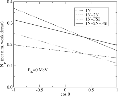
Figure 5: $N_{p}^{1N}$ (dotted line), $N_{p}^{1N+2N}$ (dashed line), $N_{p}^{1N+FSI}$ (dash-dotted line) and total $N_{p}^{1N+2N+FSI}$ (solid line), as functions of $\cos\theta$, in the the case of the OME Nijmegen89 weak transition potential.

It is clear that the $2N$ mechanism enhances the number of emitted protons at all emitted angles but having a slight preference for directions opposite to the polarization axis, hence the size of the slope of the dashed line in Fig. 5 is a little bit larger than that of the dotted line. This would increase the magnitude of the asymmetry but the larger number of protons gives finally rise to a slight decrease, as seen in Table 3. Diagrammatically speaking, we know that, for $1N$ decays, the asymmetry receives the main (negative) contribution when the proton is attached to the $\Lambda$ vertex (diagram $(a)$ of Fig. 2). The other (positive) contribution, with a neutron outgoing from the $\Lambda$ vertex (diagram $(b)$ of Fig. 2), tends to reduce the absolute value of the asymmetry. In the case of $2N$ decay diagrams, one has $npp$ and $nnp$ final states, where the proton(s) can be located at the $\Lambda$ vertex or in any of the two remaining positions. It is the increased number of positions for the final proton(s) that produces a further reduction (although small) of the asymmetry parameter. We note that the small effect of $2N$ decays on the asymmetry parameter corroborates the assumption done in al05 .

As far as FSI effects are concerned, we observe in Fig. 5 that they remove antiparallel protons and, on the other hand, more strength is added at parallel kinematics. Since the total number of protons is almost unchanged, this reduction of slope observed for the dot-dashed line also translates in a subtantial decrease in the magnitude of the asymmetry. In order to analyze further the different FSI contributions, it is convenient to write:

$$N^{FSI}_{p}(\theta)\equiv N^{2p1h}_{p}(\theta)+N^{3p2h}_{p}(\theta)\,,$$ (44)

where each of the two terms on the rhs receive contributions from each of the diagrams in Fig. 3, by cutting on $2p1h$ or $3p2h$ states, respectively. By construction, $N^{2p1h}_{p}(\theta)$ originates from a QIT between $1N$ and FSI–induced decays, while $N^{3p2h}_{p}(\theta)$ may come either from a $2N$–FSI QIT term or from a pure FSI–induced decay. The microscopic model allows us to inspect the behavior of each term. We find that the term $N^{3p2h}_{p}(\theta)$ is positive–definite and has a similar behavior to the one already discussed for $N^{2N}_{p}(\theta)$, i.e. slightly more protons are emitted antiparallel to the polarization axis. On the contrary, $N^{2p1h}_{p}(\theta)$ turns out to be negative while its kinematic behavior is very similar to the $1N$-induced decays, which produce a large negative asymmetry parameter. Therefore, the effect of the negative $N^{2p1h}_{p}(\theta)$ contributions goes in the direction of inverting this behavior, giving rise to a subtantial decrease in the size of the asymmetry or even reverting its sign, as in the case of the Nijmegen97f$+2\pi$ model.

We now pay attention to the behavior of the asymmetries of Table 3 with the enegy cut $E_{th}$. We observe that the size of the asymmetry $a_{\Lambda}^{1N+2N}$ decreases slightly for increasing $E_{th}$. This reduction can be explained from a microscopic point of view by inspecting the momentum distribution predicted by our approach for the three particles, $p_{1}$ (particle outgoing from the $\Lambda$ vertex), $p_{2}$ and $p_{3}$, stemming from $2N$ decays, shown in Fig. 12 of Ba10 . Particles are named in that figure with the same notation as in Fig. 4 of the present work. The distributions for particles $p_{1}$ and $p_{3}$ are very similar to each other and are peaked at a lower momentum than the distribution for $p_{2}$. Due to isospin reasons, the main (negative) contribution to the asymmetry is obtained when a proton is located in $p_{1}$, while protons in $p_{2}$ and/or $p_{3}$ reduce the magnitude of the asymmetry. The effect of $E_{th}$ is to reduce the importance of the particle $p_{1}$ with respect to $p_{2}$. This explains the reduction in the magnitude of $a_{\Lambda}^{{1N}+2N}$ for increasing $E_{th}$. Note, however, that the decrease is much stronger in the case of the $a_{\Lambda}^{1N+FSI}$ asymmetry, and this is also the behavior of the complete calculation, $a_{\Lambda}^{1N+2N+FSI}$. In order to understand this behavior, we recall that the energy cut removes nucleons, making $N_{p}(0^{0})+N_{p}(180^{0})$ smaller and, consequently, the magnitude of the asymmetry larger. But the final consequence of the $E_{th}$ cut on the asymmetry will be determined by whether the increase in size due to the removal of nucleons is counterbalanced by the changes in the slope $N_{p}(0^{0})-N_{p}(180^{0})$. In Fig. 6 we show the effect of this cut for $N_{p}^{1N+2N}(\theta)$ (dashed lines) and $N_{p}^{1N+2N+FSI}(\theta)$ (solid lines) as functions of $\cos\theta$, for the OME Nijmegen89 model. We clearly see a reduction in the number of protons as well as a decrease in the slope with increasing $E_{th}$ . These two effects modify the asymmetry parameter in opposite ways and the results of Table 3 show that, within our models, the reduction of the asymmetry due to the decrease in the slope dominates over the increase associated to the removal of particles. The reduction in the slope is much more pronounced for the FSI contributions. The final result is that we observe a substantial reduction in the magnitude of the asymmetry $a_{\Lambda}^{1N+2N+FSI}$ with an increasing energy cut.

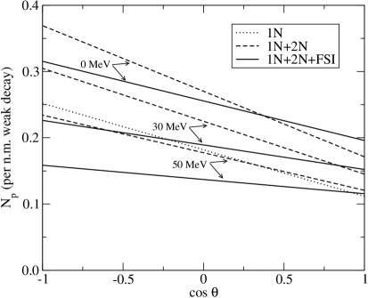
Figure 6: The functions $N_{p}^{1N+2N}$ (dashed lines) and $N_{p}^{1N+2N+FSI}$ (solid lines) for different energy cuts, $E_{th}=0$,30 and 50 MeV, in the the case of the OME Nijmegen89 weak transition potential. The dotted line corresponds to $N_{p}^{1N}$ at $E_{th}=0$ MeV.

This behavior contrasts with the INC results of al05 ; Ch07 , where, for increasing $E_{th}$, the size of the asymmetry $a^{1N+FSI}_{\Lambda}$ increases and tends to the intrinsic value. We note that the INC model for FSI originates from a semi–classical description which has an intuitive interpretation. Nucleons are tracked in their way out of the nucleus as classical particles. Sometimes a nucleon leaves the nucleus without any interaction with the medium, in other cases it scatters one or more times with the other bound nucleons. Therefore, a nucleon emerging from an elementary non–mesonic decay can change momentum, direction and charge, other nucleons can be emitted as well, etc. Clearly, the random character of these FSI processes is responsible for the strong reduction of $a^{1N+FSI}_{\Lambda}$ by about a factor two or more with respect to the intrinsic asymmetry $a^{1N}_{\Lambda}$ al05 ; Ch07 . The introduction of an energy cut $E_{th}$ affects mainly those nucleons which have suffered scattering processes. For increasing $E_{th}$, the nucleons coming from elementary decays (not affected by FSI) become dominant and the asymmetry tends to the intrinsic value. This is also reflected in Fig. 2 of al05 by the tendency of $N_{p}^{1N+FSI}(\theta)\mid_{E_{th}}$ to move towards $N_{p}^{1N}(\theta)$ as the energy cut is increased, both functions becoming very similar (in size and slope) at around $E_{th}=50$ MeV.

The situation for our microscopic approach is different as it is based on quantum mechanics, where QIT play an important role. It was shown in ba11 that the $2p1h$ and $3p2h$ terms of the proton kinetic energy spectra $N_{p}^{FSI}(T_{p})=N_{p}^{2p1h}(T_{p})+N_{p}^{3p2h}(T_{p})$ have a different behavior from each other. While $N_{p}^{3p2h}(T_{p})$ gives a positive distribution, has its maximum for $T_{p}=0$ and decreases for increasing $T_{p}$, the QIT $N^{2p1h}(T_{p})$ is a negative bell–shaped distribution with the minimum at $T_{p}\cong 80$ MeV. Thus, a non–vanishing energy cut $E_{th}$ appreciably reduces $N_{p}^{3p2h}$ while leaving $N_{p}^{2p1h}$ almost unchanged, and this later contribution is the one producing a significant decrease in the slope of $N_{p}^{1N+2N+FSI}(\theta)$. Therefore, as $E_{th}$ is increased, the magnitude of the asymmetry parameter decreases.

We end our discussion by comparing our results with experiment. The asymmetry data reported in Table 3 was obtained by KEK–E508 for a kinetic energy threshold $E_{th}$ of about 30 MeV. Despite the noticeable differences among the whole set of predictions, they are all compatible with experiment due to the large error bar of data. By considering our results for $E_{th}=30$ MeV and the central value of the experimental data, the best agreement is obtained for both Nijmegen89 and Nijmegen97f models when the two–pion–exchange potential is not included. Certainly, our calculation shows that the effect of the two–pion–exchange is very important in asymmetry calculations, but to establish definite conclusions on the effect of this potential more detailed studies are required. In general, the addition of any new contribution to the weak transition potential has to be done consistently with the rest of the potential itself (which might require some readjustment to reproduce the observables) and with the approach adopted in the calculation. However, in order to obtain fruitful information from these studies new and more precise data is needed to constrain the unknown parameters of the weak decay models.

VI Remarks and Conclusions

We have discussed a microscopic diagrammatic formalism to evaluate the asymmetry in the distribution of protons emitted in the non–mesonic decay of polarized hypernuclei. The calculation is performed in nuclear matter and then extended to finite hypernuclei (${}^{12}_{\Lambda}$C) by means of the local density approximation. Our approach takes into account both the $2N$ decay mechanism and the nucleon FSI in a unified many–body scheme. The effect of the $2N$ decays on the asymmetry parameter is evaluated here for the first time. The present work is also the first one to implement the FSI on the asymmetry parameter by means of a quantum-mechanical microscopic approach. In addition to the usual OME weak transition potentials, which we take from the Nijmegen89 and Nijmegen97f parametrizations, we have also considered the effect of the two–pion–exchange potential introduced in ji01 . We give results for both the intrinsic asymmetry parameter, $a^{1N}_{\Lambda}$, and for the asymmetry parameter modified by the $2N$-induced mechanisms and FSI effects, $a^{1N+2N+FSI}_{\Lambda}$, which is the one that can be compared to the observed asymmetry $a^{\rm M}_{\Lambda}$.

While the effect of $2N$ is predicted to be rather limited, the nucleon FSI turned out to be very important: they reduce the magnitude of the asymmetry parameter, making all the weak transition potential models adopted in this work capable of describing consistently the experimental data for $a^{\rm M}_{\Lambda}$ and for the non–mesonic weak decay rates. In particular, the large error bars in the observable asymmetry do not allow us to determine which of the two potential models, OME or OME$+2\pi$, provides the best description of the experiments.

To the best of our knowledge, the only former work which evaluated the intrinsic asymmetry in nuclear matter is due to Dubach et al. du96 , where an approximate scheme rather different from ours (neglecting $2N$ decays and nucleon FSI) was employed. The action of FSI was considered within a semi–classical description in al05 ; Ch07 , by means of an INC model. In a former calculation ba11 , it was shown that the INC model and the present microscopic approach provide similar results for the nucleon emission spectra in the non–mesonic weak decay of unpolarized $\Lambda$ hypernuclei. Our results for $a^{1N}_{\Lambda}$ and $a^{1N+FSI}_{\Lambda}$ with a vanishing proton kinetic energy cut, $E_{th}=0$, fairly agree with each other too. However, the situation changes for non–vanishing values of $E_{th}$. For increasing $E_{th}$, the negative asymmetry of the INC model increases in magnitude, while a decrease is observed in the microscopic model. One should note that the two schemes represent rather different approaches to the problem of dealing with nuclear correlations after the weak decay takes place. The microscopic model of the present work provides a reliable method that can be improved systematically. It however ignores multinucleon processes that are accounted for, semiclassically and via multi-step processes, in the INC model. To determine which is the most realistic approach, an accurate experimental determination of the asymmetry parameter, possibly exploring its $E_{th}$–dependence, would certainly be welcome.

One should always keep in mind that the main motivation in the study of the non–mesonic weak decay of hypernuclei is to extract information on strangeness–changing baryon–baryon interactions. The understanding of the $\Gamma_{n}/\Gamma_{p}$ ratio and the asymmetry parameter suggests that a fairly reasonable knowledge of non–mesonic decay has been achieved. However, we have obtained agreement with all the experimental data employing different parametrizations of the weak transition potential. Due to the lack of precise data for the asymmetry parameter, we find that the role of the two–pion–exchange mechanism, which was essential to reproduce this observable in some models Ch07 , can not even be firmly established here. In any case, what is certain is the agreement with the set of data can only be achieved after a proper development of approaches that take care of nucleon FSI. Due to the special nature of the in–medium non–mesonic weak decay, these are complex models, but they are required to establish a link between theory and experiment.

Finally, we recall that there still remains an important disagreement between theory an experiment for the hypernuclear non–mesonic weak decay: theoretical evaluations of nucleon emission spectra involving protons strongly overestimate the experimental distributions. This discrepancy may not be isolated but hidden behind the errors bars in the data for the decay rates. An additional aspect that has not yet been studied but which could lead to a non–negligible contribution to the nucleon spectra is the inclusion of the $\Delta(1232)$–resonance in our many–body Feynman diagram scheme. We intend to study this problem in the future.

Appendix

Here we present the explicit expressions needed in the evaluation of $N_{p}^{2N}(\theta)$ starting from the Feynman diagrams $pp$ and $ph$ in Fig. 3. We omit the derivation of the expressions for $N_{p}^{FSI}(\theta)$ obtained from the same diagrams, as they can be obtained from the $N_{p}^{2N}(\theta)$ ones after some simple changes: the spin–isospin structures are the same, as well as the general expressions, except for some step functions and energy denominators.

We begin with the contribution of the diagram $pp$ of Fig. 3. First, we introduce the partial, isospin–dependent decay widths for $\vec{\Lambda}np\to nnp$:

$$\Gamma^{pp,\,p_{1}}_{\tau\tau^{\prime};\tau_{N}{\tau^{\prime}}_{N}}(\mbox{\boldmath$k$},k_{F},\theta) = \frac{(G_{F}m_{\pi}^{2})^{2}}{(2\pi)^{5}}\left(\frac{f_{\pi}^{2}}{4\pi}\right)^{2}\frac{1}{m_{\pi}^{4}}\frac{2}{(2\pi)^{2}}\;\int d\mbox{\boldmath$q$}\int d\mbox{\boldmath$t$}\int d\mbox{\boldmath$h$}\int d\mbox{\boldmath$h^{\prime}$}\,\theta(q_{0})$$

$$\times\theta(|\mbox{\boldmath$k$}-\mbox{\boldmath$q$}|-k_{F})\theta(k_{F}-|\mbox{\boldmath$h$}+\mbox{\boldmath$q$}|)\,\theta(|\mbox{\boldmath$h$}-\mbox{\boldmath$t$}+\mbox{\boldmath$q$}|-k_{F})\theta(k_{F}-|\mbox{\boldmath$h$}|)$$

$$\times\theta(|\mbox{\boldmath$h^{\prime}$}+\mbox{\boldmath$t$}|-k_{F})\,\theta(k_{F}-|\mbox{\boldmath$h^{\prime}$}|)\;\delta(\cos\theta-(\mbox{\boldmath$k-q$})_{z}/|\mbox{\boldmath$k-q$}|)$$

$$\times\delta(q_{0}-(E_{N}(\mbox{\boldmath$h$}-\mbox{\boldmath$t$}+\mbox{\boldmath$q$})-E_{N}(\mbox{\boldmath$h$})+E_{N}(\mbox{\boldmath$h^{\prime}$}+\mbox{\boldmath$t$})-E_{N}(\mbox{\boldmath$h^{\prime}$}))$$

$$\times\frac{{\cal S}^{pp}_{\tau\tau^{\prime};\tau_{N}{\tau^{\prime}}_{N}}(q,t)}{(E_{N}(\mbox{\boldmath$h$}-\mbox{\boldmath$t$}+\mbox{\boldmath$q$})-E_{N}(\mbox{\boldmath$h$}+\mbox{\boldmath$q$})+E_{N}(\mbox{\boldmath$h^{\prime}$}+\mbox{\boldmath$t$})-E_{N}(\mbox{\boldmath$h^{\prime}$}))^{2}}\,,$$

$$\Gamma^{pp,\,p_{2}}_{\tau\tau^{\prime};\tau_{N}{\tau^{\prime}}_{N}}(\mbox{\boldmath$k$},k_{F},\theta) = \Gamma^{pp,\,p_{1}}_{\tau\tau^{\prime};\tau_{N}{\tau^{\prime}}_{N}}(\mbox{\boldmath$k$},k_{F},\theta)|$$

$$\delta(\cos\theta-(\mbox{\boldmath$k-q$})_{z}/|\mbox{\boldmath$k-q$}|)\rightarrow\delta(\cos\theta-(\mbox{\boldmath$h-t+q$})_{z}/|\mbox{\boldmath$h-t+q$}|)\,,$$

$$\Gamma^{pp,\,p_{3}}_{\tau\tau^{\prime};\tau_{N}{\tau^{\prime}}_{N}}(\mbox{\boldmath$k$},k_{F},\theta) = \Gamma^{pp,\,p_{1}}_{\tau\tau^{\prime};\tau_{N}{\tau^{\prime}}_{N}}(\mbox{\boldmath$k$},k_{F},\theta)|$$

$$\delta(\cos\theta-(\mbox{\boldmath$k-q$})_{z}/|\mbox{\boldmath$k-q$}|)\rightarrow\delta(\cos\theta-(\mbox{\boldmath$h^{\prime}+t$})_{z}/|\mbox{\boldmath$h^{\prime}+t$}|)\,,$$

where $p_{1}$, $p_{2}$ and $p_{3}$ indicate the position of the final proton. In a similar way, for the reaction $\vec{\Lambda}pp\rightarrow npp$ we have:

$$\Gamma^{pp,\,p_{1},\,p_{2}}_{\tau\tau^{\prime};\tau_{N}{\tau^{\prime}}_{N}}(\mbox{\boldmath$k$},k_{F},\theta) = \frac{(G_{F}m_{\pi}^{2})^{2}}{(2\pi)^{5}}\left(\frac{f_{\pi}^{2}}{4\pi}\right)^{2}\frac{1}{m_{\pi}^{4}}\frac{2}{(2\pi)^{2}}\;\int d\mbox{\boldmath$q$}\int d\mbox{\boldmath$t$}\int d\mbox{\boldmath$h$}\int d\mbox{\boldmath$h^{\prime}$}\,\theta(q_{0})$$

$$\times\theta(|\mbox{\boldmath$k$}-\mbox{\boldmath$q$}|-k_{F})\theta(k_{F}-|\mbox{\boldmath$h$}+\mbox{\boldmath$q$}|)\,\theta(|\mbox{\boldmath$h$}-\mbox{\boldmath$t$}+\mbox{\boldmath$q$}|-k_{F})\theta(k_{F}-|\mbox{\boldmath$h$}|)$$

$$\times\theta(|\mbox{\boldmath$h^{\prime}$}+\mbox{\boldmath$t$}|-k_{F})\,\theta(k_{F}-|\mbox{\boldmath$h^{\prime}$}|)$$

$$\times(\delta(\cos\theta-(\mbox{\boldmath$k-q$})_{z}/|\mbox{\boldmath$k-q$}|)+\delta(\cos\theta-(\mbox{\boldmath$h+q-t$})_{z}/|\mbox{\boldmath$h+q-t$}|))/2$$

$$\times\delta(q_{0}-(E_{N}(\mbox{\boldmath$h$}-\mbox{\boldmath$t$}+\mbox{\boldmath$q$})-E_{N}(\mbox{\boldmath$h$})+E_{N}(\mbox{\boldmath$h^{\prime}$}+\mbox{\boldmath$t$})-E_{N}(\mbox{\boldmath$h^{\prime}$}))$$

$$\times\frac{{\cal S}^{pp}_{\tau\tau^{\prime};\tau_{N}{\tau^{\prime}}_{N}}(q,t)}{(E_{N}(\mbox{\boldmath$h$}+\mbox{\boldmath$q$}-\mbox{\boldmath$t$})-E_{N}(\mbox{\boldmath$h$}+\mbox{\boldmath$q$})+E_{N}(\mbox{\boldmath$h^{\prime}$}+\mbox{\boldmath$t$})-E_{N}(\mbox{\boldmath$h^{\prime}$}))^{2}}\,,$$

$$\Gamma^{pp,\,p_{1},\,p_{3}}_{\tau\tau^{\prime};\tau_{N}{\tau^{\prime}}_{N}}(\mbox{\boldmath$k$},k_{F},\theta) = \Gamma^{pp,\,p_{1},\,p_{2}}_{\tau\tau^{\prime};\tau_{N}{\tau^{\prime}}_{N}}(\mbox{\boldmath$k$},k_{F},\theta)|$$

$$\delta(\cos\theta-(\mbox{\boldmath$h+q-t$})_{z}/|\mbox{\boldmath$h+q-t$}|)\rightarrow\delta(\cos\theta-(\mbox{\boldmath$h^{\prime}+t$})_{z}/|\mbox{\boldmath$h^{\prime}+t$}|),$$

$$\Gamma^{pp,\,p_{2},\,p_{3}}_{\tau\tau^{\prime};\tau_{N}{\tau^{\prime}}_{N}}(\mbox{\boldmath$k$},k_{F},\theta) = \Gamma^{pp,\,p_{1},\,p_{2}}_{\tau\tau^{\prime};\tau_{N}{\tau^{\prime}}_{N}}(\mbox{\boldmath$k$},k_{F},\theta)|$$

$$\delta(\cos\theta-(\mbox{\boldmath$k-q$})_{z}/|\mbox{\boldmath$k-q$}|)\rightarrow\delta(\cos\theta-(\mbox{\boldmath$h^{\prime}+t$})_{z}/|\mbox{\boldmath$h^{\prime}+t$}|)\,.$$

The next step is to implement the isospin–summation to obtain:

$$\Gamma^{pp,\,p_{1}}_{np} = 4({\Gamma}^{pp,\,p_{1}}_{11,11}+{\Gamma}^{pp,\,p_{1}}_{00,00}+2{\Gamma}^{pp,\,p_{1}}_{11,01})\,,$$ (51)

$$\Gamma^{pp,\,p_{2}}_{np} = 5{\Gamma}^{pp,\,p_{2}}_{11,11}+{\Gamma}^{pp,\,p_{2}}_{00,00}+{\Gamma}^{pp,\,p_{2}}_{11,00}+5{\Gamma}^{pp,\,p_{2}}_{00,11}$$

$$-2{\Gamma}^{pp,\,p_{2}}_{11,01}+6{\Gamma}^{pp,\,p_{2}}_{01,11}-2{\Gamma}^{pp,\,p_{2}}_{00,01}-2{\Gamma}^{pp,\,p_{2}}_{01,00}+4{\Gamma}^{pp,\,p_{2}}_{01,01}\,,$$

$$\Gamma^{pp,\,p_{3}}_{np} = 5{\Gamma}^{pp,\,p_{3}}_{11,11}+{\Gamma}^{pp,\,p_{3}}_{00,00}+{\Gamma}^{pp,\,p_{3}}_{11,00}+5{\Gamma}^{pp,\,p_{3}}_{00,11}$$

$$-2{\Gamma}^{pp,\,p_{3}}_{11,01}-6{\Gamma}^{pp,\,p_{3}}_{01,11}-2{\Gamma}^{pp,\,p_{3}}_{00,01}+2{\Gamma}^{pp,\,p_{3}}_{01,00}-4{\Gamma}^{pp,\,p_{3}}_{01,01}\,,$$

where the $(\mbox{\boldmath$k$},k_{F},\theta)$–dependence of all these functions has been omitted for simplicity. In a similar way, for the $\vec{\Lambda}pp\rightarrow npp$ reaction we have:

$$\Gamma^{pp,\,p_{1},\,p_{2}}_{pp} = 16{\Gamma}^{pp,\,p_{1},\,p_{2}}_{11,11}\,,$$ (52)

$$\Gamma^{pp,\,p_{1},\,p_{3}}_{pp} = 4({\Gamma}^{pp,\,p_{1},\,p_{3}}_{11,11}+{\Gamma}^{pp,\,p_{1},\,p_{3}}_{11,00}-2{\Gamma}^{pp,\,p_{1},\,p_{3}}_{11,01})\,,$$

$$\Gamma^{pp,\,p_{2},\,p_{3}}_{pp} = {\Gamma}^{pp,\,p_{2},\,p_{3}}_{11,11}+{\Gamma}^{pp,\,p_{2},\,p_{3}}_{00,00}+{\Gamma}^{pp,\,p_{2},\,p_{3}}_{00,11}+2{\Gamma}^{pp,\,p_{2},\,p_{3}}_{11,01}-2{\Gamma}^{pp,\,p_{2},\,p_{3}}_{01,11}$$

$$+2{\Gamma}^{pp,\,p_{2},\,p_{3}}_{00,01}-2{\Gamma}^{pp,\,p_{2},\,p_{3}}_{01,00}-4{\Gamma}^{pp,\,p_{2},\,p_{3}}_{01,01}\,.$$

The final point is to employ Eq. (23) to implement the local density approximation. We have, then:

$$\Gamma^{pp}_{np}(\theta) \equiv \Gamma^{pp,\,p_{1}}_{np}(\theta)+\Gamma^{pp,\,p_{2}}_{np}(\theta)+\Gamma^{pp,\,p_{3}}_{np}(\theta)\,,$$ (53)

$$\Gamma^{pp}_{pp}(\theta) \equiv \Gamma^{pp,\,p_{1},\,p_{2}}_{pp}(\theta)+\Gamma^{pp,\,p_{1},\,p_{3}}_{pp}(\theta)+\Gamma^{pp,\,p_{2},\,p_{3}}_{pp}(\theta)\,.$$

Finally, the $pp$ contribution to $N_{p}^{2N}(\theta)$ is obtained by Eq. (25).

We then consider the $2N$ decay contribution from the $ph$ diagram of Fig. 3. We follow the same steps of the former contributions. We start by introducing the partial, isospin–dependent decay widths for $\vec{\Lambda}np\to nnp$:

$$\Gamma^{ph,\,p_{1}}_{\tau\tau^{\prime};\tau_{N}{\tau^{\prime}}_{N}}(\mbox{\boldmath$k$},k_{F},\theta) = \frac{(G_{F}m_{\pi}^{2})^{2}}{(2\pi)^{5}}\left(\frac{f_{\pi}^{2}}{4\pi}\right)^{2}\frac{1}{m_{\pi}^{4}}\frac{2}{(2\pi)^{2}}\;\int d\mbox{\boldmath$q$}\int d\mbox{\boldmath$t$}\int d\mbox{\boldmath$h$}\int d\mbox{\boldmath$h^{\prime}$}\,\theta(q_{0})$$

$$\times\theta(|\mbox{\boldmath$k$}-\mbox{\boldmath$q$}|-k_{F})\theta(|\mbox{\boldmath$h$}-\mbox{\boldmath$t$}|-k_{F})\,\theta(|\mbox{\boldmath$h$}-\mbox{\boldmath$t$}+\mbox{\boldmath$q$}|-k_{F})\theta(k_{F}-|\mbox{\boldmath$h$}|)$$

$$\times\theta(k_{F}-|\mbox{\boldmath$h$}+\mbox{\boldmath$q$}|)\,\theta(|\mbox{\boldmath$h^{\prime}$}+\mbox{\boldmath$t$}|-k_{F})\,\theta(k_{F}-|\mbox{\boldmath$h^{\prime}$}|)\;\delta(\cos\theta-(\mbox{\boldmath$k-q$})_{z}/|\mbox{\boldmath$k-q$}|)$$

$$\times\delta(q_{0}-(E_{N}(\mbox{\boldmath$h$}-\mbox{\boldmath$t$}+\mbox{\boldmath$q$})-E_{N}(\mbox{\boldmath$h$})+E_{N}(\mbox{\boldmath$h^{\prime}$}+\mbox{\boldmath$t$})-E_{N}(\mbox{\boldmath$h^{\prime}$}))$$

$$\times\frac{{\cal S}^{ph}_{\tau\tau^{\prime};\tau_{N}{\tau^{\prime}}_{N}}(q,t)}{E_{N}(\mbox{\boldmath$h$}-\mbox{\boldmath$t$})-E_{N}(\mbox{\boldmath$h$})+E_{N}(\mbox{\boldmath$h^{\prime}$}+\mbox{\boldmath$t$})-E_{N}(\mbox{\boldmath$h^{\prime}$})}$$

$$\times\frac{1}{E_{N}(\mbox{\boldmath$h$}+\mbox{\boldmath$q$}-\mbox{\boldmath$t$})-E_{N}(\mbox{\boldmath$h$}+\mbox{\boldmath$q$})+E_{N}(\mbox{\boldmath$h^{\prime}$}+\mbox{\boldmath$t$})-E_{N}(\mbox{\boldmath$h^{\prime}$})}\,,$$

$$\Gamma^{ph,\,p_{2}}_{\tau\tau^{\prime};\tau_{N}{\tau^{\prime}}_{N}}(\mbox{\boldmath$k$},k_{F},\theta) = \Gamma^{ph,\,p_{1}}_{\tau\tau^{\prime};\tau_{N}{\tau^{\prime}}_{N}}(\mbox{\boldmath$k$},k_{F},\theta)|$$

$$\delta(\cos\theta-(\mbox{\boldmath$k-q$})_{z}/|\mbox{\boldmath$k-q$}|)\rightarrow\delta(\cos\theta-(\mbox{\boldmath$h-t+q$})_{z}/|\mbox{\boldmath$h-t+q$}|)\,,$$

$$\Gamma^{ph,\,p_{3}}_{\tau\tau^{\prime};\tau_{N}{\tau^{\prime}}_{N}}(\mbox{\boldmath$k$},k_{F},\theta) = \Gamma^{ph,\,p_{1}}_{\tau\tau^{\prime};\tau_{N}{\tau^{\prime}}_{N}}(\mbox{\boldmath$k$},k_{F},\theta)|$$

$$\delta(\cos\theta-(\mbox{\boldmath$k-q$})_{z}/|\mbox{\boldmath$k-q$}|)\rightarrow\delta(\cos\theta-(\mbox{\boldmath$h^{\prime}+t$})_{z}/|\mbox{\boldmath$h^{\prime}+t$}|)\,,$$

where $p_{1}$, $p_{2}$ and $p_{3}$ indicate the position of the emitted proton. In a similar way, for the reaction $\vec{\Lambda}pp\rightarrow npp$ we have:

$$\Gamma^{ph,\,p_{1},\,p_{3}}_{\tau\tau^{\prime};\tau_{N}{\tau^{\prime}}_{N}}(\mbox{\boldmath$k$},k_{F},\theta) = \frac{(G_{F}m_{\pi}^{2})^{2}}{(2\pi)^{5}}\left(\frac{f_{\pi}^{2}}{4\pi}\right)^{2}\frac{1}{m_{\pi}^{4}}\frac{2}{(2\pi)^{2}}\;\int d\mbox{\boldmath$q$}\int d\mbox{\boldmath$t$}\int d\mbox{\boldmath$h$}\int d\mbox{\boldmath$h^{\prime}$}\,\theta(q_{0})$$

$$\times\theta(|\mbox{\boldmath$k$}-\mbox{\boldmath$q$}|-k_{F})\theta(|\mbox{\boldmath$h$}-\mbox{\boldmath$t$}|-k_{F})\,\theta(|\mbox{\boldmath$h$}-\mbox{\boldmath$t$}+\mbox{\boldmath$q$}|-k_{F})\theta(k_{F}-|\mbox{\boldmath$h$}|)$$

$$\times\theta(|\mbox{\boldmath$h^{\prime}$}+\mbox{\boldmath$t$}|-k_{F})\,\theta(k_{F}-|\mbox{\boldmath$h^{\prime}$}|)$$

$$\times(\delta(\cos\theta-(\mbox{\boldmath$k-q$})_{z}/|\mbox{\boldmath$k-q$}|)+\delta(\cos\theta-(\mbox{\boldmath$h^{\prime}+t$})_{z}/|\mbox{\boldmath$h^{\prime}+t$}|))/2$$

$$\times\delta(q_{0}-(E_{N}(\mbox{\boldmath$h$}-\mbox{\boldmath$t$}+\mbox{\boldmath$q$})-E_{N}(\mbox{\boldmath$h$})+E_{N}(\mbox{\boldmath$h^{\prime}$}+\mbox{\boldmath$t$})-E_{N}(\mbox{\boldmath$h^{\prime}$}))$$

$$\times\frac{{\cal S}^{ph}_{\tau\tau^{\prime};\tau_{N}{\tau^{\prime}}_{N}}(q,t)}{(E_{N}(\mbox{\boldmath$h$}-\mbox{\boldmath$t$})-E_{N}(\mbox{\boldmath$h$})+E_{N}(\mbox{\boldmath$h^{\prime}$}+\mbox{\boldmath$t$})-E_{N}(\mbox{\boldmath$h^{\prime}$}))^{2}}\,,$$

$$\Gamma^{ph,\,p_{2},\,p_{3}}_{\tau\tau^{\prime};\tau_{N}{\tau^{\prime}}_{N}}(\mbox{\boldmath$k$},k_{F},\theta) = \Gamma^{ph,\,p_{1},\,p_{3}}_{\tau\tau^{\prime};\tau_{N}{\tau^{\prime}}_{N}}(\mbox{\boldmath$k$},k_{F},\theta)|$$

$$\delta(\cos\theta-(\mbox{\boldmath$k-q$})_{z}/|\mbox{\boldmath$k-q$}|)\rightarrow\delta(\cos\theta-(\mbox{\boldmath$h-t+q$})_{z}/|\mbox{\boldmath$h-t+q$}|)\,,$$

The next step is to implement the isospin summation to obtain:

$$\Gamma^{ph,\,p_{1}}_{np} = 4(-{\Gamma}^{ph,\,p_{1}}_{11,11}+{\Gamma}^{ph,\,p_{1}}_{11,00}+2{\Gamma}^{ph,\,p_{1}}_{11,01})\,,$$ (59)

$$\Gamma^{ph,\,p_{2}}_{np} = -3{\Gamma}^{ph,\,p_{2}}_{11,11}+{\Gamma}^{ph,\,p_{2}}_{00,00}+5{\Gamma}^{ph,\,p_{2}}_{00,11}+{\Gamma}^{ph,\,p_{2}}_{11,00}$$

$$+6{\Gamma}^{ph,\,p_{2}}_{01,11}-2{\Gamma}^{ph,\,p_{2}}_{01,00}-2{\Gamma}^{ph,\,p_{2}}_{11,01}-2{\Gamma}^{ph,\,p_{2}}_{00,01}+4{\Gamma}^{ph,\,p_{2}}_{01,01}\,,$$

$$\Gamma^{ph,\,p_{3}}_{np} = -3{\Gamma}^{ph,\,p_{3}}_{11,11}+{\Gamma}^{ph,\,p_{3}}_{00,00}+5{\Gamma}^{ph,\,p_{3}}_{00,11}+{\Gamma}^{ph,\,p_{3}}_{11,00}$$

$$-6{\Gamma}^{ph,\,p_{3}}_{01,11}+2{\Gamma}^{ph,\,p_{3}}_{01,00}-2{\Gamma}^{ph,\,p_{3}}_{11,01}-2{\Gamma}^{ph,\,p_{3}}_{00,01}-4{\Gamma}^{ph,\,p_{3}}_{01,01}\,,$$

where the $(\mbox{\boldmath$k$},k_{F},\theta)$–dependence of all these functions has been omitted for simplicity. In a similar way, for the $\vec{\Lambda}pp\rightarrow npp$ reaction we have:

$$\Gamma^{ph,\,p_{1},\,p_{3}}_{pp} = 4(-{\Gamma}^{ph,\,p_{1},\,p_{3}}_{11,11}+{\Gamma}^{ph,\,p_{1},\,p_{3}}_{11,00}-2{\Gamma}^{ph,\,p_{1},\,p_{3}}_{11,01})\,,$$ (60)

$$\Gamma^{ph,\,p_{2},\,p_{3}}_{pp} = {\Gamma}^{ph,\,p_{2},\,p_{3}}_{11,11}+{\Gamma}^{ph,\,p_{2},\,p_{3}}_{00,00}+{\Gamma}^{ph,\,p_{2},\,p_{3}}_{00,11}+{\Gamma}^{ph,\,p_{2},\,p_{3}}_{11,00}-2{\Gamma}^{ph,\,p_{2},\,p_{3}}_{01,11}$$

$$-2{\Gamma}^{ph,\,p_{2},\,p_{3}}_{01,00}+2{\Gamma}^{ph,\,p_{2},\,p_{3}}_{11,01}+2{\Gamma}^{ph,\,p_{2},\,p_{3}}_{00,01}-4{\Gamma}^{ph,\,p_{2},\,p_{3}}_{01,01}\,,$$

One thus has to perform the local density approximation, through Eq. (23), to obtain:

$$\Gamma^{ph}_{np}(\theta) \equiv \Gamma^{ph,\,p_{1}}_{np}(\theta)+\Gamma^{ph,\,p_{2}}_{np}(\theta)+\Gamma^{ph,\,p_{3}}_{np}(\theta)\,,$$ (61)

$$\Gamma^{ph}_{pp}(\theta) \equiv \Gamma^{ph,\,p_{1},\,p_{3}}_{pp}(\theta)+\Gamma^{ph,\,p_{2},\,p_{3}}_{pp}(\theta)\,,$$

and finally the $ph$ contribution to $N_{p}^{2N}(\theta)$ is obtained by Eq. (25).

References

- (1) W. M. Alberico and G. Garbarino, Phys. Rep. 369 (2002) 1; in Hadron Physics, IOS Press, Amsterdam, 2005, p. 125. Edited by T. Bressani, A. Filippi and U. Wiedner. Proceedings of the International School of Physics “Enrico Fermi”, Course CLVIII, Varenna (Italy), June 22 – July 2, 2004.
- (2) A. Parreño, Lect. Notes Phys. 724 (2007) 141.
- (3) S. Ajimura et al., Phys. Lett. B 282 (1992) 293; Phys. Rev. Lett. 84 (2000) 4052.
- (4) H. Bandō, T. Motoba, J. Z̆ofka, Int. J. Mod. Phys. A 5 (1990) 4021.
- (5) J. F. Dubach, G. B. Feldman, B. R. Holstein and L. de la Torre, Ann. Phys. 249 (1996) 146.
- (6) A. Parreño, A. Ramos and C. Bennhold, Phys. Rev. C 56 (1997) 339.
- (7) A. Parreño and A. Ramos, Phys. Rev. C 65 (2001) 015204.
- (8) C. Barbero, A. P. Galeão and F. Krmpotić, Phys. Rev. C 72 (2005) 035210.
- (9) W. M. Alberico, G. Garbarino, A. Parreño and A. Ramos, Phys. Rev. Lett. 94 (2005) 082501.
- (10) C. Barbero, A. P. Galeao and F. Krmpotic, Phys. Rev. C 76 (2007) 054321.
- (11) K. Sasaki, T. Inoue, M. Oka, Nucl. Phys. A 669 (2000) 331; Nucl. Phys. A 678 (2000) 455, Erratum; Nucl. Phys. A 707 (2002) 477.
- (12) A. Parreño, C. Bennhold and B. R. Holstein, Phys. Rev. C 70 (2004) 051601(R).
- (13) K. Sasaki, M. Izaki and M. Oka, Phys. Rev. C 71 (2005) 035502.
- (14) C. Barbero and A. Mariano, Phys. Rev. C 73 (2006) 024309.
- (15) C. Chumillas, G. Garbarino, A. Parreño and A. Ramos, Phys. Lett. B 657 (2007) 180.
- (16) E. Oset, H. Toki, M. Mizobe and T. T. Takahashi, Prog. Theor. Phys. 103 (2000) 351.
- (17) D. Jido, E. Oset and J. E. Palomar Nucl. Phys. A 694 (2001) 525.
- (18) E. Bauer and G. Garbarino, Phys. Rev. C 81 (2010) 064315.
- (19) G. Garbarino, A. Parreño, and A. Ramos, Phys. Rev. Lett. 91 (2003) 112501; Phys. Rev. C 69 (2004) 054603.
- (20) E. Bauer and G. Garbarino, Phys. Lett. B 698 (2011) 306.
- (21) E. Bauer, G. Garbarino, A. Parreño and A. Ramos, Nucl. Phys. A 836 (2010) 199.
- (22) E. Bauer, Nucl. Phys. A781 (2007) 424; ibid A 796 (2007) 11.
- (23) E. Bauer, Nucl. Phys. A 796 (2007) 11.
- (24) J. Bystricky, F. Lehar and P. Winternitz, Jour. de Phys. 39 (1978) 1.
- (25) A. Ramos, E. van Meijgaard, C. Bennhold and B. K. Jennings, Nucl. Phys. A 544 (1992) 703.
- (26) E. Bauer and F. Krmpotić, Nucl. Phys. A 717 (2003) 217.
-
(27)
M. N. Nagels, T. A. Rijken and J. J. de Swart,
Phys. Rev. D 15 (1977) 2547;
P. M. M. Maessen, T. A. Rijken and J. J. de Swart, Phys. Rev. C 40 (1989) 2226. - (28) V. G. J. Stoks and Th. A. Rijken, Phys. Rev. C 59 (1999) 3009; Th. A. Rijken, V. G. J. Stoks and Y. Yamamoto, ibid. 59 (1999) 21.
- (29) R. Machleidt, K. Holinde and Ch. Elster; Phys. Rep. 149 (1987) 1.
- (30) M. B. Barbaro, A. De Pace, T. W. Donnelly and A. Molinari, Nucl. Phys. A 596 (1996) 553.
- (31) O. Hashimoto and H. Tamura, Prog. Part. Nucl. Phys. 57 (2006) 564, and references therein.
- (32) M. Kim et al., Phys. Rev. Lett. 103 (2009) 182502.
- (33) M. Agnello et al., Phys. Lett. B 685 (2010) 247.
- (34) M. Agnello et al., Phys. Lett. B 701 (2011) 556.
- (35) T. Maruta et al., Eur. Phys. J. A 33 (2007) 255.
- (36) C. Chumillas, A. Parreño and A. Ramos, in preparation.