Nonperturbative study of the four-point heavy quark Green’s functions in Coulomb gauge

Abstract:

The heavy quark sector of Coulomb gauge QCD is investigated, by making a heavy quark mass expansion of the QCD action and restricting to the leading order. With the truncation of the Yang-Mills sector to include only dressed two-point functions, we study the Dyson-Schwinger equations for the four-point quark Green’s functions (proper and amputated). In this limit, we provide an exact solution for the four-point quark Green’s functions and show that the corresponding poles relate to the bound state energy of the heavy quark system. Moreover, a natural separation between the physical and unphysical poles in the Green’s functions emerges.

1 Introduction

Coulomb gauge is a suitable choice for investigating the confinement phenomenon, as in this gauge the Gribov-Zwanziger scenario becomes distinctly prominent: the temporal component of the gluon propagator provides the long range confining potential, whereas the spatial propagator is infrared suppressed [1]. On the other hand, traditional studies of the heavy quark sector of quantum chromodynamics (QCD) mainly use phenomenologically motivated potentials in the place of the Yang-Mills sector. In this context, it is appropriate to investigate the relationship between the nonperturbative scale associated with confinement and the Yang-Mills sector of the theory.

This talk reviews results obtained in the heavy quark limit of Coulomb gauge QCD [2, 3]. After making an expansion in the heavy quark mass and restricting to the leading order, we consider the heavy quark propagator and the homogeneous Bethe-Salpeter equation for quark-antiquark systems. With the further truncation to exclude pure Yang-Mills vertices (but retaining nonperturbative dressed propagators), we show that the rainbow-ladder approximation is exact in this case and we establish a connection between the temporal gluon propagator and the external physical scale (the string tension), at least within the leading order truncation. In the second part of the talk, we investigate the (full nonperturbative) four-point quark-antiquark Green’s functions. We present exact, analytic solutions, and show that the physical poles of the Green’s function explicitly separate from the possible unphysical ones. Moreover, we find that the physical poles of the Bethe-Salpeter equation are contained within the singularities of the Green’s function. These results will hopefully be useful in the future investigations of phenomenological models for mesons and baryons (see, for example, Ref. [4] for a numerical analysis of the inhomogeneous Bethe-Salpeter equation).

2 Quark propagator in the heavy mass limit

Let us start by considering the explicit quark contribution to the full QCD generating functional:

$$Z[\overline{\chi},\chi] = \int{\cal D}\Phi\exp{\left\{\imath\int d^{4}x\overline{q}_{\alpha}(x)\left[\imath\gamma^{0}D_{0}+\imath{\vec{\gamma}}\!\cdot\!{\vec{D}}-m\right]_{\alpha\beta}q_{\beta}(x)\right\}}$$ (1)

$$\times\exp{\left\{\imath\int d^{4}x\left[\overline{\chi}_{\alpha}(x)q_{\alpha}(x)+\overline{q}_{\alpha}(x)\chi_{\alpha}(x)\right]+\imath{\cal S}_{YM}\right\}}.$$

In the above, ${\cal D}\Phi$ denotes the integration over all fields present, $q_{\alpha}$ is the quark field, $\bar{q}_{\alpha}$ the conjugate antiquark field, and $\bar{\chi}_{\alpha},\chi_{\alpha}$ the corresponding sources. The common index $\alpha,\beta\dots$ denotes the color, spin and flavor indices. The Dirac $\gamma$ matrices satisfy $\left\{\gamma^{\mu},\gamma^{\nu}\right\}=2g^{\mu\nu}$, with the metric $g^{\mu\nu}=\textrm{diag}(1,-\vec{1})$. The structure constants of the $SU(N_{c})$ group are denoted with $f^{abc}$, and the Hermitian generators satisfy $[T^{a},T^{b}]=\imath f^{abc}T^{c}$ and are normalized via $\textrm{Tr}(T^{a},T^{b})=\delta^{ab}/2$. ${\cal S}_{YM}$ represents the Yang-Mills part of the action and

$$D_{0}=\partial_{0}-\imath gT^{a}\sigma^{a}(x),\,\,\,\,\,\,\vec{D}=\vec{\nabla}+\imath gT^{a}\vec{A}^{a}(x),$$ (2)

are the temporal and spatial components of the covariant derivative in the fundamental color representation ($\vec{A}$ and $\sigma$ refer to the spatial and temporal components of the gluon field, respectively).

We now decompose the full quark field according to the heavy quark transformation

$$q_{\alpha}(x)=e^{-\imath mx_{0}}\left[h(x)+H(x)\right]_{\alpha},\;h_{\alpha}(x)=e^{\imath mx_{0}}\left[\frac{{\mathbf{1}}+\gamma^{0}}{2}q(x)\right]_{\alpha},\;H_{\alpha}(x)=e^{\imath mx_{0}}\left[\frac{{\mathbf{1}}-\gamma^{0}}{2}q(x)\right]_{\alpha}$$ (3)

(similarly for the antiquark field), where the two components $h$ and $H$ are introduced with the help of the spinor projectors $(1\pm\gamma^{0})/2$. This is a particular case of the heavy quark transform, adopted from the Heavy Quark Effective Theory [HQET] [5], which turns out to be useful in Coulomb gauge.

After inserting the quark fields, decomposed according to Eq. (3), into the generating functional Eq. (1), we integrate out the $H$-fields and make an expansion in the inverse of the heavy quark mass (in the following, we will adopt the standard terminology and denote it simply “mass expansion”). At leading order, the generating functional reduces to:

$$Z[\overline{\chi},\chi] = \int{\cal D}\Phi\exp{\left\{\imath\int d^{4}x\overline{h}_{\alpha}(x)\left[\imath\partial_{0x}+gT^{a}\sigma^{a}(x)\right]_{\alpha\beta}h_{\beta}(x)\right\}}$$ (4)

$$\times\exp{\left\{\imath\int d^{4}x\left[e^{-\imath mx_{0}}\overline{\chi}_{\alpha}(x)h_{\alpha}(x)+e^{\imath mx_{0}}\overline{h}_{\alpha}(x)\chi_{\alpha}(x)\right]+\imath{\cal S}_{YM}\right\}}+{\cal O}\left(1/m\right),$$

where we have replaced the covariant derivative $D_{0}$ with its explicit expression. In the above expression, we notice that as a result of the heavy quark transformation, at leading order in the mass expansion the quark interacts only with the temporal gluon, whereas the spatial component is suppressed. Also, note the absence of the Dirac $\gamma$ structure, as a result of the multiplication with the projectors $({\mathbf{1}}\pm\gamma^{0})/2$ (physically, this implies that the spin degree of freedom decouples from the system). A further important point is that in Eq. (4) we have kept the full quark and antiquark sources, as opposed to HQET, where the sources corresponding to the large components $h$ are used. This means that at leading order in the mass expansion we are allowed to use the full apparatus of the functional formalism, and hence derive the full Dyson-Schwinger equations in Coulomb gauge QCD, while replacing the corresponding propagators and vertices by their leading order expressions.

In Coulomb gauge QCD (without the mass expansion), the quark gap equation for the proper two-point function is given by (see Ref. [6] for a complete derivation and notation):

$$\Gamma_{\overline{q}q\alpha\gamma}(k) =\Gamma_{\overline{q}q\alpha\gamma}^{(0)}(k) +\!\int\!\,\,\,\raisebox{-1.72218pt}{\large$\bar{}$}\!\!d\,{\omega}\,\left\{\Gamma_{\overline{q}q\sigma\alpha\beta}^{(0)a}(k,-\omega,\omega-k)W_{\overline{q}q\beta\kappa}(\omega)\Gamma_{\overline{q}q\sigma\kappa\gamma}^{b}(\omega,-k,k-\omega)W_{\sigma\sigma}^{ab}(k-\omega)\right.$$ (5)

$$\left.\!+\Gamma_{\overline{q}qA\alpha\beta i}^{(0)a}(k,-\omega,\omega-k)W_{\overline{q}q\beta\kappa}(\omega)\Gamma_{\overline{q}qA\kappa\gamma j}^{b}(\omega,-k,k-\omega)W_{AAij}^{ab}(k-\omega)\right\}\!,$$

where $\,\,\,\raisebox{-1.72218pt}{\large$\bar{}$}\!\!d\,{\omega}\,=d\omega/(2\pi)^{4}$. In order to solve this equation, we first need to specify the tree-level quark proper two-point function and the components of the tree-level quark-gluon vertex. They are derived directly from the generating functional Eq. (4) and are given by:

$$\Gamma_{\overline{q}q\alpha\beta}^{(0)}(k)=\imath\delta_{\alpha\beta}\left[k_{0}-m\right]+{\cal O}\left(1/m\right),$$ (6)

$$\Gamma_{\overline{q}q\sigma\alpha\beta}^{(0)a}(k_{1},k_{2},k_{3})=\left[gT^{a}\right]_{\alpha\beta}+{\cal O}\left(1/m\right).$$ (7)

Note that the spatial component of the quark-gluon vertex is of order ${\cal O}(1/m)$, as shall be explained shortly below. Further, the nonperturbative temporal gluon propagator entering Eq. (5) has the form [7]:

$$W_{\sigma\sigma}^{ab}(k)=\delta^{ab}W_{\sigma\sigma}(\vec{k})=\delta^{ab}\frac{\imath}{\vec{k}^{2}}D_{\sigma\sigma}(\vec{k}^{2}).$$ (8)

Following lattice results, which signal that that the gluon dressing function is largely independent of energy, we assume that $D_{\sigma\sigma}$ is a function of the three-momentum. Also, lattice investigations indicate that $D_{\sigma\sigma}$ is infrared divergent and behaves like $1/\vec{k}^{2}$ for vanishing $\vec{k}^{2}$ [8] (however, we will need the explicit form of this function only at the end of the calculation).

Finally, the last input is provided by the Slavnov-Taylor identity, which furnishes a relation between the two- and three-point functions of the theory. This is derived from the invariance of the QCD action under a time-dependent Gauss-BRST transform [2], and in Coulomb gauge reads ($k_{1}+k_{2}+k_{3}=0$):

$$k_{3}^{0}\Gamma_{\overline{q}q\sigma\alpha\beta}^{d}(k_{1},k_{2},k_{3}) = \imath\frac{k_{3i}}{\vec{k}_{3}^{2}}\Gamma_{\overline{q}qA\alpha\beta i}^{a}(k_{1},k_{2},k_{3})\Gamma_{\overline{c}c}^{ad}(-k_{3})$$ (9)

$$+\Gamma_{\overline{q}q\alpha\delta}(k_{1})\left[\tilde{\Gamma}_{\overline{q};\overline{c}cq}^{d}(k_{1}+q_{0},k_{3}-q_{0};k_{2})+\imath gT^{d}\right]_{\delta\beta}$$

$$+\left[\tilde{\Gamma}_{q;\overline{c}c\overline{q}}^{d}(k_{2}+q_{0},k_{3}-q_{0};k_{1})-\imath gT^{d}\right]_{\alpha\delta}\Gamma_{\overline{q}q\delta\beta}(-k_{2}).$$

In the above, $q_{0}$ is an arbitrary energy injection scale (arising from the noncovariance of Coulomb gauge [9]), $\Gamma_{\overline{c}c}$ is the ghost proper two-point function, and $\tilde{\Gamma}_{\overline{q};\overline{c}cq}$ and $\tilde{\Gamma}_{q;\overline{c}c\overline{q}}$ are ghost-quark kernels associated with the time-dependent Gauss-BRST transform. Since in the generating functional, Eq. (4), the tree-level spatial quark-gluon vertex appears at ${\cal O}(1/m)$, by making the further truncation to neglect the pure Yang-Mills vertices, it follows from the Dyson-Schwinger equation for the spatial quark-gluon vertex that the fully dressed $\Gamma_{\bar{q}qA}\sim{\cal O}(1/m)$ (and hence it is neglected). Further, the ghost-gluon vertices involve pure Yang-Mills vertices and hence are also truncated out. Thus, in our truncation scheme and at leading order in the mass expansion, the Slavnov-Taylor identity takes the simple form:

$$k_{3}^{0}\Gamma_{\overline{q}q\sigma\alpha\beta}^{d}(k_{1},k_{2},k_{3})=\Gamma_{\overline{q}q\alpha\delta}(k_{1})\left[\imath gT^{d}\right]_{\delta\beta}-\left[\imath gT^{d}\right]_{\alpha\delta}\Gamma_{\overline{q}q\delta\beta}(-k_{2})+{\cal O}\left(1/m\right).$$ (10)

Collecting the above results, we find the following expression for the heavy quark propagator, as a solution of Eq. (5), combined with Eq. (10):

$$W_{\overline{q}q\alpha\beta}(k)=\frac{-\imath\delta_{\alpha\beta}}{\left[k_{0}-m-{\cal I}_{r}+\imath\varepsilon\right]}+{\cal O}\left(1/m\right),$$ (11)

with the constant (implicitly regularized, as indicated by the index “$r$”):

$${\cal I}_{r}=\frac{1}{2}g^{2}C_{F}\int_{r}\frac{\,\,\,\raisebox{-1.72218pt}{\large$\bar{}$}\!\!d\,{\vec{\omega}}\,D_{\sigma\sigma}(\vec{\omega})}{\vec{\omega}^{2}}+{\cal O}\left(1/m\right),$$ (12)

where $\,\,\,\raisebox{-1.72218pt}{\large$\bar{}$}\!\!d\,{\vec{\omega}}\,=d^{3}\vec{\omega}/(2\pi)^{3}$ and $C_{F}=(N_{c}^{2}-1)/2N_{c}$. The gap equation, Eq. (5), has been solved under the assumption that the temporal integral has been performed first, with the spatial integral regularized and finite. The solution, Eq. (11), is then inserted into the Slavnov-Taylor identity, Eq. (10), and we find that the temporal quark-gluon vertex remains nonperturbatively bare:

$$\Gamma_{\overline{q}q\sigma\alpha\beta}^{a}(k_{1},k_{2},k_{3})=\left[gT^{a}\right]_{\alpha\beta}+{\cal O}\left(1/m\right).$$ (13)

Note that the quark propagator, Eq. (11), possesses a single pole in the complex $k_{0}$ plane, in contrast with the standard QCD propagator, which has a double covariant pole. Hence, we need to derive the quark and antiquark propagators separately, with the corresponding Feynman prescriptions. Examining the closed quark loops (virtual quark-antiquark pairs connected by a primitive vertex), we find that they vanish due to the energy integration over two quark propagators with the same Feynman prescription, and this implies that the theory is quenched in the heavy mass limit:

$$\int\frac{dk_{0}}{\left[k_{0}-m-{\cal I}_{r}+\imath\varepsilon\right]\left[k_{0}+p_{0}-m-{\cal I}_{r}+\imath\varepsilon\right]}=0.$$ (14)

Further, note that the propagator Eq. (11) is diagonal in the outer product of the fundamental color, flavor and spinor spaces, and this exhibits the decoupling of the spin from the heavy quark system. Finally, it is important to emphasize that the position of the pole has no physical meaning, since not the propagator itself, but the bound state of a quark and an antiquark is physical. The fact that the poles in the quark propagator are shifted to infinity once the regularization is removed simply means that an infinite energy is needed to create a single quark from the vacuum. If a hadronic state is considered, only the relative energy (derived from the homogeneous Bethe-Salpeter equation) is required to describe the system, and in this case the singularities appearing in Eq. (11) cancel. Similar types of cancellation appear in the solutions of the four-point quark-antiquark Green’s function (see also the discussion from section 4).

For the antiquark propagator we obtain:

$$W_{q\overline{q}\alpha\beta}(k)=\frac{-\imath\delta_{\alpha\beta}}{\left[k_{0}+m-{\cal I}_{r}+\imath\varepsilon\right]}+{\cal O}\left(1/m\right),$$ (15)

and the corresponding temporal antiquark-gluon vertex is given by:

$$\Gamma_{q\overline{q}\sigma\alpha\beta}^{a}(k_{1},k_{2},k_{3})=-\left[gT^{a}\right]_{\beta\alpha}+{\cal O}\left(1/m\right).$$ (16)

In the above, notice the Feynman prescription of the propagator, as well as the sign of the loop correction, ${\cal I}_{r}$. As shall be discussed in the next section, this apparently minor modification will play an important role in the interpretation of the solutions of the Bethe-Salpeter equation for quark-antiquark states as bound state/confining solutions.

3 Homogeneous Bethe-Salpeter equation

Let us now consider the full homogeneous Bethe-Salpeter equation for quark-antiquark bound states [2] (see also Fig. 1):

$$\Gamma(p;P)_{\alpha\beta}=-\int\,\,\,\raisebox{-1.72218pt}{\large$\bar{}$}\!\!d\,{k}\,K_{\alpha\beta;\delta\gamma}(p,k;P)\left[W_{\overline{q}q}(k_{+})\Gamma(k;P)W_{\overline{q}q}(k_{-})\right]_{\gamma\delta}.$$ (17)

In the above, the momenta of the quarks are given by $p_{+}=p+\xi P$, $p_{-}=p-(1-\xi)P$ (similarly for $k_{\pm}$), and $\xi$ is the momentum sharing fraction (note that the solutions here and in the next section turn out to be independent of $\xi$, just as in the covariant case [10]). $P$ represents the 4-momentum of the bound state (assuming that a solution exists), $\Gamma$ is the Bethe-Salpeter vertex function for the particular bound state and $K$ is the Bethe-Salpeter kernel, which still needs to be specified.

It is well-known that the Bethe-Salpeter kernel $K$ and the quark self-energy are related via the axialvector Ward-Takahashi identity [11]. Under truncation, it was seen in the last section that the heavy quark self-energy reduces to the rainbow truncated form; the corresponding truncation for the kernel is the ladder approximation. In [2], this has been explicitly derived. The Bethe-Salpeter kernel in the heavy quark-antiquark system under the truncation considered here is thus:

$$K_{\alpha\beta;\delta\gamma}(p,k)=\Gamma_{\bar{q}q\sigma\alpha\gamma}^{a}(p_{+},-k_{+},k-p)W_{\sigma\sigma}^{ab}(\vec{p}-\vec{k})\Gamma_{q\bar{q}\sigma\beta\delta}^{bT}(-p_{-},k_{-},p-k).$$ (18)

We now insert the nonperturbative results for the propagators and vertices, Eqs. (11,13, 15,16) and the expression Eq. (8) for the temporal gluon propagator. After explicitly identifying the antiquark contribution, i.e. $W_{\overline{q}q}(k_{-})=-W_{q\overline{q}}^{T}(-k_{-})$, we perform the temporal integration over the quark and antiquark propagators, which now leads to (unlike Eq. (14)):

$$\frac{\imath}{2\pi}\int_{-\infty}^{\infty}\frac{dk_{0}}{\left[k_{+}^{0}-m-{\cal I}_{r}+\imath\varepsilon\right]\left[k_{-}^{0}-m+{\cal I}_{r}-\imath\varepsilon\right]}=\frac{-1}{{P_{0}-2\cal I}_{r}+2\imath\varepsilon}.$$ (19)

Figure 1: Homogeneous Bethe-Salpeter equation for quark-antiquark bound states. Internal propagators are fully dressed and solid lines represent the quark propagator. The box represents the Bethe-Salpeter kernel $K$ and filled blobs represent the Bethe-Salpeter vertex function $\Gamma$ with the (external) bound state leg given by a dashed line.

Further, we insert the expression Eq. (12) for ${\cal I}_{r}$ and after Fourier transforming to coordinate space we find the following solution for the bound state energy of the quark-antiquark system:

$$P_{0}=g^{2}\int_{r}\frac{\,\,\,\raisebox{-1.72218pt}{\large$\bar{}$}\!\!d\,{\vec{\omega}}\,D_{\sigma\sigma}(\vec{\omega})}{\vec{\omega}^{2}}\left[C_{F}-e^{\imath\vec{\omega}\cdot\vec{x}}C_{M}\right]+{\cal O}\left(1/m\right).$$ (20)

In the above, $C_{M}$ is an (unknown) color factor assigned to the Bethe-Salpeter vertex $\Gamma$, which has to be yet identified:

$$\left[T^{a}\Gamma(\vec{x})T^{a}\right]_{\alpha\beta}=C_{M}\Gamma_{\alpha\beta}(\vec{x}).$$ (21)

Because the total color charge of the system is conserved and vanishing [12], a quark cannot exist as an asymptotic state. Hence, the bound state energy $P_{0}$ of a quark-antiquark system can be either infinite, such that the system is not allowed, or linearly rising, if the system is confined. If the temporal gluon propagator is more infrared divergent than $1/|\vec{\omega}|$, we find that in order to ensure the convergence of the spatial integral, $C_{M}$ must be equal to $C_{F}$. This immediately leads to the condition

$$\Gamma_{\alpha\gamma}(\vec{x})=\delta_{\alpha\gamma}\Gamma(\vec{x}),$$ (22)

which implies that the Bethe-Salpeter equation can only have a finite solution for color singlet states. Further, if we assume that in the infrared $D_{\sigma\sigma}=X/\vec{\omega}^{2}$ (as indicated by the lattice [8]), where $X$ is a combination of constants, then from Eq. (20) we find

$$P_{0}\equiv\sigma|\vec{x}|=\frac{g^{2}C_{F}X}{8\pi}|\vec{x}|+{\cal O}\left(1/m\right).$$ (23)

This result shows that there is a direct connection between the physical string tension $\sigma$ and the nonperturbative Yang-Mills sector of QCD, at least under the truncation scheme employed here, which corresponds to a color singlet bound state of a quark and an antiquark, and otherwise the system has infinite energy.

4 Four-point quark-antiquark Green’s functions

Similar to the gap equation, we derive the the full Dyson-Schwinger equation for the proper (1PI) four-point quark-antiquark Green’s function in configuration space (see Ref. [3] for notation and technical details of the functional derivation):

$$<\!\!{\imath\overline{q}_{\alpha x}\imath q_{\gamma z}\imath\overline{q}_{\tau w}\imath q_{\eta t}}\!\!>=[g\gamma^{0}T^{a}]_{\alpha\beta}\int dy\,\delta(x-y)\times$$

$$\left\{\left[<\!\!{\imath\overline{\chi}_{\beta x}\imath\chi_{\kappa}}\!\!><\!\!{\imath\overline{q}_{\kappa}\imath q_{\gamma z}\imath\sigma^{c}_{\lambda}}\!\!><\!\!{\imath\rho^{c}_{\lambda}\imath\rho^{d}_{\delta}}\!\!>\right]\!\left[<\!\!{\imath\overline{q}_{\tau w}\imath q_{\nu}\imath\sigma^{b}_{\mu}}\!\!><\!\!{\imath\overline{\chi}_{\nu}\imath\chi_{\varepsilon}}\!\!><\!\!{\imath\overline{q}_{\varepsilon}\imath q_{\eta t}\imath\sigma^{d}_{\delta}}\!\!><\!\!{\imath\rho^{b}_{\mu}\imath\rho^{a}_{y}}\!\!>\right]\right.$$

$$-\left[<\!\!{\imath\overline{\chi}_{\beta x}\imath\chi_{\delta}}\!\!><\!\!{\imath\overline{q}_{\delta}\imath q_{\eta t}\imath\sigma^{c}_{\varepsilon}}\!\!><\!\!{\imath\rho^{c}_{\varepsilon}\imath\rho^{d}_{\kappa}}\!\!>\right]\!\left[<\!\!{\imath\overline{q}_{\tau w}\imath q_{\nu}\imath\sigma^{b}_{\mu}}\!\!><\!\!{\imath\overline{\chi}_{\nu}\imath\chi_{\lambda}}\!\!><\!\!{\imath\overline{q}_{\lambda}\imath q_{\gamma z}\imath\sigma^{d}_{\kappa}}\!\!><\!\!{\imath\rho^{b}_{\mu}\imath\rho^{a}_{y}}\!\!>\right]$$

$$-\left[<\!\!{\imath\overline{\chi}_{\beta x}\imath\chi_{\kappa}}\!\!><\!\!{\imath\overline{q}_{\kappa}\imath q_{\gamma z}\imath\sigma^{c}_{\lambda}}\!\!><\!\!{\imath\rho^{c}_{\lambda}\imath\rho^{d}_{\nu}}\!\!><\!\!{\overline{q}_{\tau w}\imath q_{\eta t}\imath\sigma^{d}_{\nu}\imath\sigma^{b}_{\mu}}\!\!><\!\!{\imath\rho^{b}_{\mu}\imath\rho^{a}_{y}}\!\!>\right]$$

$$+\left[<\!\!{\imath\overline{\chi}_{\beta x}\imath\chi_{\delta}}\!\!><\!\!{\imath\overline{q}_{\delta}\imath q_{\eta t}\imath\sigma^{c}_{\varepsilon}}\!\!><\!\!{\imath\rho^{c}_{\varepsilon}\imath\rho^{d}_{\kappa}}\!\!>\right]\!\left[<\!\!{\imath\overline{q}_{\tau w}\imath q_{\gamma z}\imath\sigma^{d}_{\kappa}\imath\sigma^{b}_{\lambda}}\!\!><\!\!{\imath\rho^{b}_{\lambda}\imath\rho^{a}_{y}}\!\!>\right]$$

$$+\left[<\!\!{\imath\overline{\chi}_{\beta x}\imath\chi_{\kappa}}\!\!><\!\!{\imath\overline{q}_{\kappa}\imath q_{\gamma z}\imath\overline{q}_{\tau w}\imath q_{\eta t}\sigma^{b}_{\lambda}}\!\!><\!\!{\imath\rho^{b}_{\lambda}\imath\rho^{a}_{y}}\!\!>\right]$$

$$-\left[<\!\!{\imath\overline{\chi}_{\beta x}\imath\chi_{\kappa}}\!\!><\!\!{\imath\overline{q}_{\kappa}\imath q_{\gamma z}\imath\overline{q}_{\lambda}\imath q_{\eta t}}\!\!><\!\!{\imath\overline{q}_{\tau w}\imath q_{\nu}\imath\sigma^{b}_{\mu}}\!\!><\!\!{\imath\overline{\chi}_{\nu}\imath\chi_{\lambda}}\!\!><\!\!{\imath\rho^{b}_{\mu}\imath\rho^{a}_{y}}\!\!>\right]$$

$$-\left[<\!\!{\imath\overline{\chi}_{\beta x}\imath\chi_{\kappa}}\!\!><\!\!{\imath\overline{q}_{\kappa}\imath q_{\gamma z}\imath\overline{q}_{\tau w}\imath q_{\lambda}}\!\!><\!\!{\imath\overline{\chi}_{\lambda}\imath\chi_{\delta}}\!\!><\!\!{\imath\overline{q}_{\delta}\imath q_{\eta t}\imath\sigma^{b}_{\varepsilon}}\!\!><\!\!{\imath\rho^{b}_{\varepsilon}\imath\rho^{a}_{y}}\!\!>\right]$$

$$-\left[<\!\!{\imath\overline{\chi}_{\beta x}\imath\chi_{\nu}}\!\!><\!\!{\imath\overline{q}_{\nu}\imath q_{\mu}\imath\overline{q}_{\tau w}\imath q_{\eta t}}\!\!><\!\!{\imath\overline{\chi}_{\mu}\imath\chi_{\kappa}}\!\!><\!\!{\imath\overline{q}_{\kappa}\imath q_{\gamma z}\imath\sigma^{b}_{\lambda}}\!\!><\!\!{\imath\rho^{b}_{\lambda}\imath\rho^{a}_{y}}\!\!>\right]$$

$$+\left[<\!\!{\imath\overline{\chi}_{\beta x}\imath\chi_{\kappa}}\!\!><\!\!{\imath\overline{q}_{\kappa}\imath q_{\gamma z}\imath\sigma^{c}_{\lambda}}\!\!><\!\!{\imath\rho^{c}_{\lambda}\imath\rho^{d}_{\nu}}\!\!>\right]\!\left[<\!\!{\imath\overline{q}_{\tau w}\imath q_{\mu}\imath\sigma^{d}_{\nu}}\!\!><\!\!{\imath\overline{\chi}_{\mu}\imath\chi_{\delta}}\!\!><\!\!{\imath\overline{q}_{\delta}\imath q_{\eta t}\imath\sigma^{b}_{\varepsilon}}\!\!><\!\!{\imath\rho^{b}_{\varepsilon}\imath\rho^{a}_{y}}\!\!>\right]$$

$$-\left.\left[<\!\!{\imath\overline{\chi}_{\beta x}\imath\chi_{\delta}}\!\!><\!\!{\imath\overline{q}_{\delta}\imath q_{\eta t}\imath\sigma^{c}_{\varepsilon}}\!\!><\!\!{\imath\rho^{c}_{\varepsilon}\imath\rho^{d}_{\nu}}\!\!>\right]\!\!\left[<\!\!{\imath\overline{q}_{\tau w}\imath q_{\mu}\imath\sigma^{d}_{\nu}}\!\!><\!\!{\imath\overline{\chi}_{\mu}\imath\chi_{\kappa}}\!\!><\!\!{\imath\overline{q}_{\kappa}\imath q_{\gamma z}\imath\sigma^{b}_{\lambda}}\!\!><\!\!{\imath\rho^{b}_{\lambda}\imath\rho^{a}_{y}}\!\!>\right]\right\}$$

$$+\dots$$ (24)

where the dots represent the $\vec{A}$ vertex terms (which will be truncated out in our scheme), and we have already replaced the tree-level temporal quark-gluon vertex with its expression Eq. (13). The above equation is diagrammatically represented in Fig. 2.

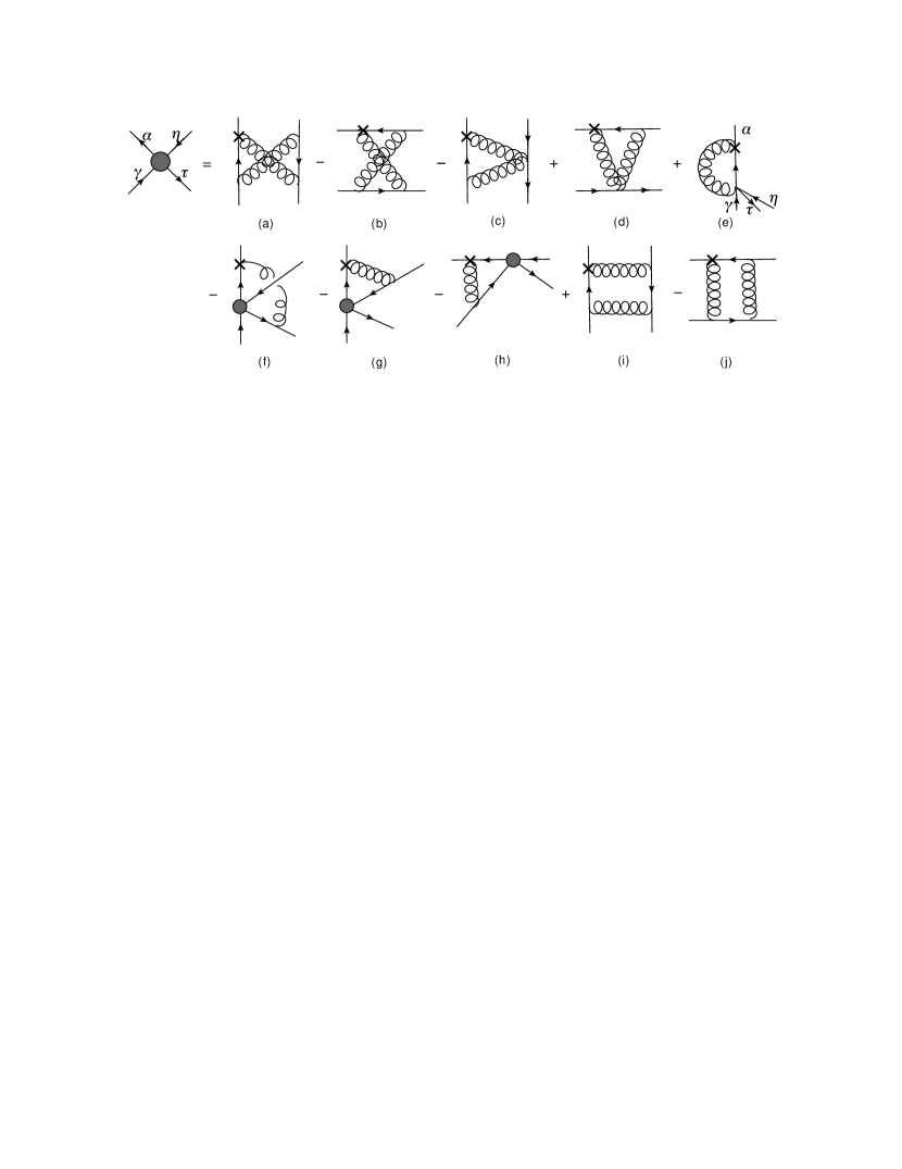
Figure 2: Diagrammatic representation of the Dyson-Schwinger equation for the 1PI 4-point quark-antiquark Green’s function. Blobs represent dressed proper (1PI) 4-point vertex, solid lines represent the quark propagator, springs denote either spatial ($\vec{A}$) or temporal ($\sigma$) gluon propagator and cross denotes the tree level quark-gluon vertex. Internal propagators and 1PI vertices are fully dressed.

We now proceed by applying our truncation scheme at leading order in the mass expansion. Since we shall consider the flavor non-singlet Green’s function in the $s$-channel (the quark and the antiquark are regarded as two distinct flavors, but with equal masses), the diagrams (a), (c) and (i) of Fig. 2 are excluded. In the diagram (b) (crossed ladder type exchange diagram), we insert as before the appropriate propagators Eqs. (11, 15) and vertices Eqs. (13, 16). The resulting energy integral is similar to the integral (2.14) and vanishes, just like the higher order contributions to the kernel of the homogeneous Bethe-Salpeter equation. Turning to the diagram (d), we see that this contribution involves a quark-two gluon vertex. From the corresponding Slavnov-Taylor identity (derived explicitly in Ref. [3]), it can be seen that this vertex is zero and hence the diagram (d) vanishes.

At this stage, we adopt the following strategy: discard for the moment the diagrams (f) and (g), which include the 1PI four-point quark-antiquark Green’s function, and the diagram (e), containing a four-quark-gluon vertex, solve the equation with the remaining terms (the diagram (h) and the rainbow-ladder term (j)), and with the obtained solution return to the diagrams (f), (g) and (e), and show that they cancel (and hence our assumption is consistent). In this case, Eq. (24) reduces to the Dyson-Schwinger equation for the 1PI four-point quark Green’s function in the $s$-channel, in the ladder-approximation (shown diagrammatically in Fig. 3):

$$\Gamma^{(4)}_{\alpha\gamma\tau\eta}(p_{1},p_{2},p_{3},p_{4})=$$ (25)

$$-\int\,\,\,\raisebox{-1.72218pt}{\large$\bar{}$}\!\!d\,{\omega}\,\left[\Gamma_{\bar{q}q\sigma\alpha\beta}^{(0)a}(p_{1},-p_{1}-\omega,\omega)W_{\bar{q}q\beta\delta}(p_{1}+\omega)\Gamma_{\bar{q}q\sigma\delta\eta}^{c}(p_{1}+\omega,p_{4},-p_{1}-p_{4}-\omega)\right]$$

$$\times\left[\Gamma_{\bar{q}q\sigma\tau\mu}^{d}(p_{3},p_{2}-\omega,p_{1}+p_{4}+\omega)W_{\bar{q}q\mu\kappa}(\omega-p_{2})\Gamma_{\bar{q}q\sigma\kappa\gamma}^{b}(\omega-p_{2},p_{2},-\omega)\right]$$

$$\times W_{\sigma\sigma}^{ab}(-\omega)W_{\sigma\sigma}^{cd}(p_{1}+p_{4}+\omega)$$

$$-\int\,\,\,\raisebox{-1.72218pt}{\large$\bar{}$}\!\!d\,{\omega}\,\Gamma_{\bar{q}q\sigma\alpha\beta}^{(0)a}(p_{1},-p_{1}-\omega,\omega)W_{\bar{q}q\beta\nu}(p_{1}+\omega)\Gamma^{(4)}_{\nu\mu\tau\eta}(p_{1}+\omega,p_{2}-\omega,p_{3},p_{4})W_{\bar{q}q\mu\kappa}(\omega-p_{2})$$

$$\times\Gamma_{\bar{q}q\sigma\kappa\gamma}^{b}(\omega-p_{2},p_{2},-\omega)W_{\sigma\sigma}^{ab}(-\omega).$$

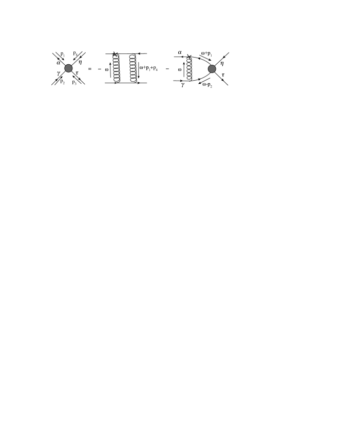
Figure 3: Truncated Dyson-Schwinger equation for the 1PI 4-point Green’s function in the $s$-channel. Same conventions as in Fig. 2 apply.

As before, we identify the antiquark component of Eq. (25) (lower line of Fig. 3) and insert the expressions Eqs. (11, 15), for the quark and antiquark propagators, along with the vertices Eqs. (13, 16) and the definition Eq. (8) for the temporal gluon propagator. We further make the assumption that $\Gamma^{(4)}(p_{1},p_{2},p_{3},p_{4})=\Gamma^{(4)}(P_{0};\vec{p}_{1}+\vec{p}_{4})$, where $P_{0}=p_{1}^{0}+p_{2}^{0}$, which allows us to separate the three-momentum and energy integrals. The energy integrals are similar to Eq. (19) and can be carried out. Making the following color decomposition for the function $\Gamma^{(4)}$:

$$\Gamma^{(4)}_{\alpha\gamma\tau\eta}=\delta_{\alpha\gamma}\delta_{\tau\eta}\Gamma_{1}^{(4)}+\delta_{\alpha\eta}\delta_{\tau\gamma}\Gamma_{2}^{(4)},$$ (26)

where $\Gamma^{(4)}_{1}$ and $\Gamma^{(4)}_{2}$ are scalar functions and Fourier transforming back to coordinate space, we find the following solution for the 1PI quark-antiquark Green’s function:

$$\Gamma^{(4)}_{\alpha\gamma\tau\eta}(P_{0};x) = \imath\left(\frac{g^{2}}{2N_{c}}\right)^{2}\frac{W_{\sigma\sigma}(x)^{2}}{P_{0}-2{\cal I}_{r}+\imath\frac{g^{2}}{2N_{c}}W_{\sigma\sigma}(x)+2\imath\varepsilon}$$ (27)

$$\times\left\{\delta_{\alpha\gamma}\delta_{\tau\eta}\frac{(P_{0}-2{\cal I}_{r})N_{c}(N_{c}^{2}-2)+\imath g^{2}N_{c}C_{F}W_{\sigma\sigma}(x)}{P_{0}-2{\cal I}_{r}-\imath g^{2}C_{F}W_{\sigma\sigma}(x)+2\imath\varepsilon}+\delta_{\alpha\eta}\delta_{\tau\gamma}\right\},$$

where $x=|\vec{x}|$ is the separation associated with the momentum $\vec{p}_{1}+\vec{p}_{4}$.

As promised, with the solution Eq. (27) for the 1PI Green’s function, we now return to the diagrams (f), (g) and (e) and show that they do not contribute to the final result. To see this, we first consider the diagram (g) and notice that the energy dependence of the internal four-point function can be written as

$$\Gamma^{(4)}(P_{0}+\omega_{0})\sim\frac{\omega_{0}^{m}}{\left[\omega_{0}+X+\imath\varepsilon\right]^{n}},$$ (28)

where $X$ is a combination of constants, $n=1,2$ and $m=0,1$. Then the energy integral takes the form

$$\int\,\,\,\raisebox{-1.72218pt}{\large$\bar{}$}\!\!d\,{\omega_{0}}\,\omega_{0}^{m}\prod_{i=1}^{2+n}\frac{1}{\left[\omega_{0}+X_{i}+\imath\varepsilon\right]}=0.$$ (29)

Clearly, this integral is a generalization of Eq. (14) and this vanishes, just as for the loop corrections in the kernel of the Bethe-Salpeter equation from the previous section and the diagram (b) from above. An identical calculation for the diagram (f), recalling that the lower line corresponds to an antiquark propagator, leads us to the fact that this integral is also zero. Finally, turning to the diagram (e), containing the four quark-gluon vertex, we notice that the perturbative series of this diagram coincides with the ladder resummation of the diagrams (f) and (g), which we have found to be vanishing, and hence this diagram is also zero (even though the five-point interaction vertex itself does not vanish – see also Ref. [3] for a detailed diagrammatic analysis). In turn, this implies that our original assumption is correct and the solution Eq. (27) is valid at every order in perturbation theory. Marginally, we note that the fact that the five-point function is finite relates to the existence of three-quark bound states in the Faddeev equation, in the ladder approximation [13].

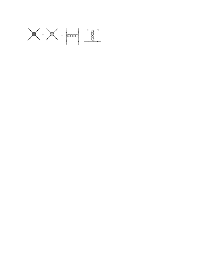
Figure 4: Relation between the 1PI (dark blob) and amputated (shaded blob) 4-point Greens function for the quark-antiquark system. Internal propagators and 1PI vertices are fully dressed.

Let us now consider the Dyson-Schwinger equation for the fully amputated four-point quark-antiquark Green’s function in the $s$-channel, which we denote $G^{(4)}$. This is related to the 1PI function $\Gamma^{(4)}$ via the Legendre transform (see Fig. 4). This study is motivated by the fact that this equation reduces (under truncation) to the inhomogeneous ladder Bethe-Salpeter equation, from which the homogeneous Bethe-Salpeter equation of the previous section is derived. In the following, we will derive the solutions of this equation, analyze the positions of the poles, and explicitly verify that the physical solutions coincide with the bound state solutions of the homogeneous Bethe-Salpeter equation.

Figure 5: Truncated Dyson-Schwinger equation for the fully amputated quark-antiquark 4-point Green’s function in the $s$-channel.

Starting with Eq. (25) (in coordinate space) for the proper function, we replace the 1PI function $\Gamma^{(4)}$ with the amputated function $G^{(4)}$ according to Fig. 4, and cut the external quark legs. The resulting equation for $G^{(4)}$ reads (see also Fig. 5):

$$G^{(4)}_{\alpha\gamma;\tau\eta}(p_{+},p_{-};k_{+},k_{-})=W_{\sigma\sigma}^{ab}(\vec{p}-\vec{k})\left[\Gamma_{\bar{q}q\sigma}^{a}\right]_{\alpha\eta}\left[\Gamma_{\bar{q}q\sigma}^{b}\right]_{\tau\gamma}$$

$$-\int\,\,\,\raisebox{-1.72218pt}{\large$\bar{}$}\!\!d\,{q}\,\left[\Gamma_{\bar{q}q\sigma}^{a(0)}W_{\bar{q}q}(q_{+})\right]_{\alpha\kappa}\left[W_{\bar{q}q}(q_{-})\Gamma_{\bar{q}q\sigma}^{b}\right]_{\mu\gamma}W_{\sigma\sigma}^{ab}(\vec{p}-\vec{q})G^{(4)}_{\kappa\mu;\tau\eta}(q_{+},q_{-};k_{+},k_{-}).$$ (30)

In the above, for the quark momenta we use the same conventions as in the Bethe-Salpeter equation, Eq. (17). Again, we replace the heavy quark and antiquark propagators and vertices with the expressions Eqs. (11, 15, 13, 16), perform the energy integration, and Fourier transform back to coordinate space. Similar to the proper four-point function, we make a color decomposition of the function $G^{(4)}$:

$$G^{(4)}_{\alpha\gamma;\tau\eta}=\delta_{\alpha\gamma}\delta_{\tau\eta}G^{(4)}_{1}+\delta_{\alpha\eta}\delta_{\tau\gamma}G^{(4)}_{2},$$ (31)

($G^{(4)}_{1}$ and $G^{(4)}_{2}$ are scalar functions), and after using the Fierz identity to sort out the color factors, we obtain the final result for the function $G^{(4)}$:

$$G^{(4)}_{\alpha\gamma;\tau\eta}(P_{0};x) =\frac{g^{2}}{2}\frac{\left(P_{0}-2{\cal I}_{r}\right)W_{\sigma\sigma}(x)}{P_{0}-2{\cal I}_{r}+\imath\frac{g^{2}}{2N_{c}}W_{\sigma\sigma}(x)+2\imath\varepsilon}$$ (32)

$$\times\left[\delta_{\alpha\gamma}\delta_{\tau\eta}\frac{(P_{0}-2{\cal I}_{r})}{P_{0}-2{\cal I}_{r}-\imath g^{2}C_{F}W_{\sigma\sigma}(x)+2\imath\varepsilon}-\delta_{\alpha\eta}\delta_{\tau\gamma}\frac{1}{N_{c}}\right],$$

where $P_{0}=p_{+}-p_{-}$ is the total energy of the $\bar{q}q$ state.

Analyzing the structure of the four-point functions, we first notice that even though the results, Eqs. (27, 32), are derived under truncation, the denominator structure of the 1PI and amputated Green’s functions are identical in both color channels, and furthermore, the physical and nonphysical singularities have disentangled automatically. Using the form Eq. (8) for the temporal gluon propagator, the denominator factor of the color singlet channel in either Eq. (27) or Eq. (32) can be rewritten in the form

$$P_{0}-g^{2}\int_{r}\frac{\,\,\,\raisebox{-1.72218pt}{\large$\bar{}$}\!\!d\,{\vec{\omega}}\,D_{\sigma\sigma}(\vec{\omega})}{\vec{\omega}^{2}}C_{F}\left[1-e^{\imath\vec{\omega}\cdot\vec{x}}\right].$$ (33)

In this expression we recognize the bound state (infrared confining) energy $P_{0\;res}(x)=\sigma|\vec{x}|$ (further assuming that $D_{\sigma\sigma}(\vec{\omega}^{2})\sim 1/\vec{\omega}^{2}$), similar to Eq. (20) for the homogeneous Bethe-Salpeter equation in the color-singlet channel. Hence, we have found an explicit analytical dependence of the four-point Green’s function on the $\bar{q}q$ bound state energy resulting from the homogeneous Bethe-Salpeter equation.

Turning to the overall denominator factors of Eqs. (27, 32), i.e. the denominator factor not specific to the color-singlet channel, we again insert the explicit form of the temporal gluon propagator and arrive at the following result:

$$P_{0}-g^{2}\int_{r}\frac{\,\,\,\raisebox{-1.72218pt}{\large$\bar{}$}\!\!d\,{\vec{\omega}}\,D_{\sigma\sigma}(\vec{\omega})}{\vec{\omega}^{2}}\left[C_{F}+\frac{1}{2N_{c}}e^{\imath\vec{\omega}\cdot\vec{x}}\right].$$ (34)

This factor does not appear in the homogeneous Bethe-Salpeter equation; it is part of the normalization and, similar to the quark propagator, represents an unphysical pole which is shifted to infinity when the (implicit) regularization is removed.

5 Conclusions

In this talk, we have discussed the Dyson-Schwinger and Bethe-Salpeter equations for quark-antiquark systems in Coulomb gauge, at leading order in the heavy quark mass expansion and with the truncation to include only the (nonperturbative) temporal gluon propagator. Under this truncation, the rainbow approximation to the quark gap equation is exact, as is the corresponding ladder approximation to the homogeneous Bethe-Salpeter equation. The only physical solution corresponds to confinement, i.e. only color singlet meson states have finite energy (and hence are physically allowed), and otherwise the system has infinite energy. Incidentally, these results are supported by recent Dyson-Schwinger studies in Coulomb gauge at leading order [14].

Turning to the four-point quark-antiquark Green’s functions, we have presented analytic solutions for both the proper and amputated Green’s functions. The two functions have the same denominator structures, and the physical and nonphysical singularities disentangle, the physical poles coinciding with the bound state solutions obtained for the homogeneous Bethe-Salpeter equation.

References

• [1] V. N. Gribov, Quantization of non-Abelian gauge theories, Nucl. Phys. B 139 (1978) 1; D. Zwanziger, Lattice Coulomb Hamiltonian and static color-Coulomb field, Nucl. Phys.  B 485, 185 (1997); D. Zwanziger, Renormalization in the Coulomb gauge and order parameter for confinement in QCD, Nucl. Phys. B 518 (1998) 237.
• [2] C. Popovici, P. Watson and H. Reinhardt, Coulomb gauge confinement in the heavy quark limit, Phys. Rev.  D 81 (2010) 105011.
• [3] C. Popovici, P. Watson and H. Reinhardt, Higher order heavy quark Green’s functions in Coulomb gauge, Phys. Rev. D 83 (2011) 125018 [arXiv:1103.4786 [hep-ph]].
• [4] M. Blank and A. Krassnigg, Matrix algorithms for solving (in)homogeneous bound state equations, Comput. Phys. Commun.  182 (2011) 1391 [arXiv:1009.1535 [hep-ph]].
• [5] M. Neubert, Heavy quark symmetry, Phys. Rept.  245 (1994) 259.
• [6] C. Popovici, P. Watson and H. Reinhardt, Quarks in Coulomb gauge perturbation theory, Phys. Rev.  D 79, 045006 (2009).
• [7] P. Watson and H. Reinhardt, Two-Point Functions of Coulomb Gauge Yang-Mills Theory, Phys. Rev.  D 77, 025030 (2008) [arXiv:0709.3963 [hep-th]].
• [8] M. Quandt, G. Burgio, S. Chimchinda and H. Reinhardt, Coulomb gauge ghost propagator and the Coulomb potential, PoS CONFINEMENT8, 066 (2008).
• [9] P. Watson and H. Reinhardt, Slavnov-Taylor identities in Coulomb gauge Yang-Mills theory, Eur. Phys. J.  C 65 (2010) 567.
• [10] R. Alkofer, P. Watson and H. Weigel, Mesons in a Poincare covariant Bethe-Salpeter approach, Phys. Rev. D 65 (2002) 094026 [hep-ph/0202053].
• [11] S. L. Adler and A. C. Davis, Chiral Symmetry Breaking in Coulomb Gauge QCD, Nucl. Phys. B 244 (1984) 469.
• [12] H. Reinhardt, P. Watson, Resolving temporal Gribov copies in Coulomb gauge Yang-Mills theory, Phys. Rev.  D79 (2009) 045013.
• [13] C. Popovici, P. Watson and H. Reinhardt, Three-quark confinement potential from the Faddeev equation, Phys. Rev. D 83 (2011) 025013 [arXiv:1010.4254 [hep-ph]].
• [14] P. Watson and H. Reinhardt, Leading order infrared quantum chromodynamics in Coulomb gauge, arXiv:1111.6078 [hep-ph].