Half-vortex sheets and domain-wall trains of rotating two-component Bose-Einstein condensates in spin-dependent optical lattices

Abstract

We investigate half-vortex sheets and domain-wall trains of rotating two-component Bose-Einstein condensates in spin-dependent optical lattices. The two-component condensates undergo phase separation in the form of stripes arranged alternatively. The vortices of one component are aligned in lines in the low-density regions and filled with the other component, which results in a stable vortex configuration, straight half-vortex sheets. A train of novel domain walls, with spatially periodic “eyebrow-like” spin textures embedded on them, are formed at the interfaces of the two components. We reveal that these spatially periodic textures on the domain walls result from the linear gradient of the relative phase, which is induced by the alternating arrangement of the vortex sheets in the two components. An accurate manipulation of the textures can be realized by adjusting the intercomponent interaction strength, the rotating angular frequency and the period of the optical lattices.

I Introduction

In recent years, the study on topological defects has become a fascinating topic in Bose-Einstein condensates (BECs). In a single-component BEC, topological defects manifest themselves as integer vortices single-component ; Freilich ; Jezek ; Wang . Multi-component BECs, which are described by a vector order parameter, allow the existence of more variety of exotic topological defects, such as fractional vortices multi-component ; Semenoff ; Ji ; Eto ; Su , domain walls multi-component ; Sadler and textures multi-component ; Yi ; Huhtamaki ; Kawakami ; Su2 . As the simplest example of the multi-component condensates, two-component BECs have also attracted much interest to study various topological defects.

There are various vortex configurations in rotating two-component BECs, such as triangular vortex lattices, rectangular vortex lattices, vortex sheets, rotating droplets and giant vortices Mueller ; Kasamatsu ; Schweikhard ; Woo ; Yang ; Kasamatsu2 ; Mason . Different configurations depend on the intracomponent interaction, the intercomponent interaction and the particle numbers. Especially, when the intercomponent interaction is strong enough and the imbalance of the intracomponent parameter is small, “serpentine” vortex sheets can be formed Kasamatsu ; Kasamatsu2 . However, this configuration is disordered and not well controlled. Although straight vortex sheets were also discussed in the previous work Woo ; Kasamatsu2 , stable ones have never been obtained. This is because there exist different metastable vortex sheet configurations with almost the same energy as the straight one.

Due to the spin degrees of freedom, the two-component BECs can be considered as a novel magnetic material. When the condensates undergo phase separation, domain walls are formed naturally at the interfaces of the two components. There have been several studies of domain walls in two-component BECs Coen ; Son ; Garcia ; Kevrekidis ; Malomed ; Takeuch ; Jin . Most of them concentrate on the formation and dynamics of domain walls, while the internal structure of domain walls has not been explored so much. In contrast, in common magnetic materials, various internal structures of domain walls have been extensively investigated both theoretically and experimentally (see, e.g., Ref. Lee and references therein). In order to study domain walls in two-component BECs, phase separation is required. Usually, phase separation is realized by the strong intercomponent repulsion. As the experimental realization of the spin-dependent optical lattices Mandel ; McKay , the two-component condensates can be separated in an arbitrary form, which provides us a well-controlled platform to study domain walls.

A variety of spin textures are discovered in two-component BECs, such as skyrmions Battye , meron-pairs Kasamatsu3 and spin-2 textures Ruben . The motifs of different textures always correspond to different vortex configurations. For example, an axisymmetric vortex and a nonaxisymmetric one correspond to a skyrmion and a meron-pair, respectively Kasamatsu4 , and a spin-2 texture corresponds to a pair of vortices with opposite sign that reside in different components Ruben . This suggests that it is a feasible method to produce novel textures by controlling the arrangement of the vortices.

In this paper, we investigate topological defects of rotating two-component BECs in spin-dependent optical lattices. We find that this system supports a new stable vortex configuration, straight half-vortex sheets. A train of novel domain walls are formed at the interfaces of the two components. We concentrate on their unique internal structures, and find that spatially periodic “eyebrow-like” spin textures are embedded on the domain walls. We reveal that these spatially periodic textures are directly determined by the arrangement of the straight half-vortex sheets. The influences of the system parameters on the textures are also investigated both analytically and numerically. Our results show that the number of the textures on a wall is proportional to the rotating angular frequency and the period of the optical lattices, and with the increase of the intercomponent interaction strength, the textures become thinner and thinner. This allows us to make an accurate manipulation of the textures.

This paper is organized as follows. In Sec. II, we give the model of the rotating two-component BECs in spin-dependent optical lattices. In Sec. III, we study the stable straight half-vortex sheets, and discuss the discontinuity of the tangential component of the superfluid velocity across the sheet. In Sec. IV, we investigate the internal structures of the domain walls and reveal the formation mechanism of the spatially periodic “eyebrow-like” spin textures. In Sec. V, we focus on the texture control. We conclude this paper in Sec. VI.

II The Model

We consider a two-level ${}^{\text{87}}$Rb BEC system with $\left|F=1,m_{f}=-1\right\rangle\equiv\left|1\right\rangle$ and $\left|F=2,m_{f}=1\right\rangle\equiv\left|2\right\rangle$ Mertes . In the weak interaction limit, the two-component condensates in a frame rotating at an angular frequency $\Omega$ around the $z$ axis can be described by the coupled Gross-Pitaevskii (GP) equations

$$i\hbar\frac{\partial\Psi_{i}\left(\mathbf{r},t\right)}{\partial t} = \Bigl{[}-\frac{\hbar^{2}}{2m}\mathbf{\nabla}^{2}+V_{\text{H}}+\sum_{j=1,2}g_{ij}\left|\Psi_{j}\right|^{2}$$ (1)

$$+V_{\text{OL}i}-\Omega\hat{L}_{z}\Bigr{]}\Psi_{i}\left(\mathbf{r},t\right),$$

where $\Psi_{i}$ is the macroscopic wave function of the $i$th component ($i=1,2$). $g_{ij}=4\pi\hbar^{2}a_{ij}/m$ represents the strength of interatomic interactions characterized by the intra- and intercomponent $s$-wave scattering lengths $a_{ij}$ and the mass $m$ of an atom. $\hat{L}_{z}=-i\hbar\left(x\partial_{y}-y\partial_{x}\right)$ is the $z$-component of the angular momentum operator. The external potential consists of two parts, the harmonic trapping potential $V_{\text{H}}=\frac{1}{2}m\left[\omega_{\bot}^{2}\left(x^{2}+y^{2}\right)+\omega_{z}^{2}z^{2}\right]$ and the spin-dependent optical lattice potential $V_{\text{OL}i}$, where $V_{\text{OL}1}=I_{0}\sin^{2}(kx)$ and $V_{\text{OL}2}=I_{0}\cos^{2}(kx)$. Here $k$ is the wave vector of the laser light used for the optical lattice potentials and $I_{0}$ is the potential depth of the lattices. The wave functions are normalized as $\sum_{i}\int\left|\Psi_{i}\right|^{2}d\mathbf{r}=N$, where $N$ is the total number of condensate atoms.

For simplicity, we assume that the harmonic trapping frequencies satisfy $\omega_{z}\gg\omega_{\bot}$. Then, the condensates are pressed into a “pancake”. This allows us to reduce Eq. (1) to a two-dimensional form as Kasamatsu5

$$i\hbar\frac{\partial\psi_{i}\left(x,y,t\right)}{\partial t} = \Bigl{[}-\frac{\hbar^{2}}{2m}\mathbf{\nabla}^{2}+\tilde{V}_{\text{H}}+\sum_{j=1,2}\eta g_{ij}\left|\psi_{j}\right|^{2}$$ (2)

$$+V_{\text{OL}i}-\Omega\hat{L}_{z}\Bigr{]}\psi_{i}\left(x,y,t\right),$$

where $\eta=\left(h/m\omega_{z}\right)^{-1/2}$ is a reductive parameter. The two-dimensional wave functions are normalized as $\sum_{i}\int\left|\psi_{i}\right|^{2}dxdy=N$. The harmonic trapping potential is reduced to its 2D form $\tilde{V}_{\text{H}}=\frac{1}{2}m\omega_{\bot}^{2}\left(x^{2}+y^{2}\right)$, where the tilde will be omitted in the following for simplicity.

In order to describe the system more clearly, the intuitive pictures of the external potentials are presented in Figs. 1(a)–1(f). Experimentally, the spin-dependent optical lattice potentials $V_{\text{OL}1}$ and $V_{\text{OL}2}$ can be realized by employing two counter-propagating blue-detuned laser beams with the same frequency but perpendicular linear polarization vectors Mandel . A schematic of the spin-dependent optical lattices is presented in Fig. 1(g).

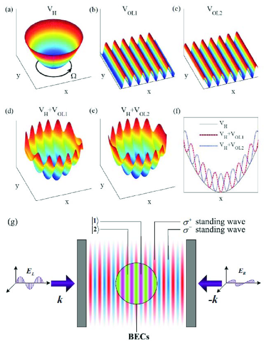
Figure 1: (Color online) (a) The harmonic trapping potential $V_{\text{H}}$ is rotated about the $z$ axis at a frequency $\Omega$. (b) The spin-dependent optical lattice potential $V_{\text{OL}1}=I_{0}\sin^{2}\left(kx\right)$, which is experienced by the $\left|1\right\rangle$ state. (c) The spin-dependent optical lattice potential $V_{\text{OL}2}=I_{0}\cos^{2}\left(kx\right)$, which is experienced by the $\left|2\right\rangle$ state. (d) The composite potential $V_{\text{H}}+V_{\text{OL}1}$. (e) The composite potential $V_{\text{H}}+V_{\text{OL}2}$. (f) Cross sections of $V_{\text{H}}$ (solid line), $V_{\text{H}}+V_{\text{OL}1}$ (dashed line) and $V_{\text{H}}+V_{\text{OL}2}$ (dotted line) along the $x$ axis. (g) Schematic of the spin-dependent optical lattices. Two polarized standing wave laser fields $\sigma^{+}$ (red) and $\sigma^{-}$ (blue) are formed by two counter-propagating blue-detuned laser beams with the same frequency but perpendicular linear polarization vectors. This gives rise to the optical lattice potentials $V_{\text{OL}1}$ and $V_{\text{OL}2}$, which are experienced by the $\left|1\right\rangle$ state (pink) and the $\left|2\right\rangle$ state (green), respectively.

In our simulations, the ${}^{\text{87}}$Rb atoms are assigned to the two states equally and the total number of them is $N=10^{5}$. The radial and axial trapping frequencies are $\omega_{\bot}=2\pi\times 15$ Hz and $\omega_{z}=2\pi\times 150$ Hz, respectively. We use the scattering lengths Mertes : $a_{11}=100.40a_{0},a_{22}=95.00a_{0}$ and $a_{12}=a_{21}=97.66a_{0}$ ($a_{0}$ is the Bohr radius), except when we discuss the influence of the intercomponent interaction on the textures in Sec. V. The intensity of the laser light used for the optical lattice potentials is chosen as $I_{0}=k_{B}\times 27.5$ nK ($k_{B}$ is the Boltzmann’s constant) Burger , which is powerful enough such that the two states are phase separated.

III Half-vortex sheets

In this section, we present a stable vortex configuration, straight half-vortex sheets. By using the imaginary-time propagation method Bao , we solve Eq. (2) numerically and obtain the ground state of the two-component condensates. The density profiles with the rotating angular frequency $\Omega=0.6\omega_{\bot}$ and the period of the optical lattice potential $T=\pi\xi$ are presented in Fig. 2, where $\xi=\left(\hbar/m\omega_{\bot}\right)^{-1}$ is the spatial scale. All the vortices are denoted by crosses ($\times$), whose positions are determined by the singularities of the phase. From Fig. 2, we can see that the two-component condensates undergo phase separation in the form of stripes arranged alternatively. The vortices of one component are aligned in lines in the low-density regions and filled with the other component. This results in alternatively arranged straight vortex sheets in the two components. Obviously, all the positions of the vortices in one component are vortex-free regions in the other component, so all the vortices are half quantized Ji ; Eto ; Su . We refer to this vortex configuration as straight half-vortex sheets. Even though the half-vortex sheets do not influence the total density distribution of the condensates, they are crucial for the formation of the spatially periodic spin textures on the domain walls.

In the absence of the spin-dependent optical lattices, the straight vortex sheets configuration has also been discussed in the phase-separated region Woo ; Kasamatsu2 . However, this configuration is ustable in that case, and there exist many different shapes of metastable vortex sheet configurations with almost the same energy as the straight one. This is because the energy of the vortex sheets is mainly determined by the intervortex spacing within a vortex sheet and the intersheet spacing rather than the shape of the vortex sheets. In contrast, when the spin-dependent optical lattices are present, the shape of the vortex sheets becomes an important factor in determining the energy. Any bending in the straight vortex sheets will cost much energy, so the straight half-vortex sheets configuration obtained in our system is stable. In our imaginary-time propagations, for any trial initial configurations, the straight vortex sheets configuration is always uniquely obtained after sufficient convergence of the energy.

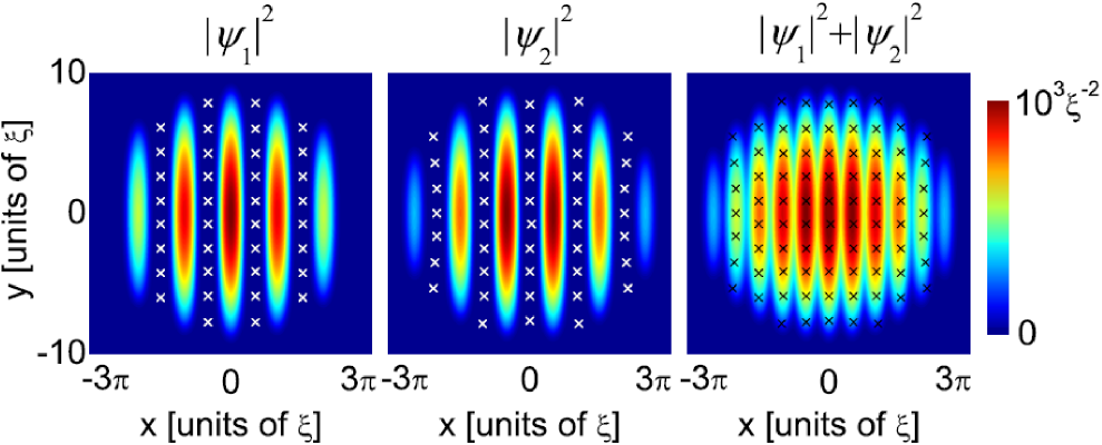
Figure 2: (Color online) The ground state density profiles of $\left|\psi_{1}\right|^{2}$, $\left|\psi_{2}\right|^{2}$ and $\left|\psi_{1}\right|^{2}+\left|\psi_{2}\right|^{2}$ for the rotating angular frequency $\Omega=0.6\omega_{\bot}$ and the period of the optical lattice potential $T=\pi\xi$ with $\xi=\left(\hbar/m\omega_{\bot}\right)^{1/2}$. The locations of the vortices are marked by crosses ($\times$).

The most well-known character of a vortex sheet is the discontinuity of the tangential component of the velocity across the sheet. The regular arrangement of the straight vortex sheets allows us to observe this phenomenon clearly. In Fig. 3(a), the tangential components (the components along the $y$ axis) $v_{1y}$ and $v_{2y}$ of the superfluid velocities $\mathbf{v}_{1}$ and $\mathbf{v}_{2}$  of the two states are presented. We can see that both $v_{1y}$ and $v_{2y}$ discontinuously jump across every sheet. In order to describe the tangential velocities in detail, the section views of $v_{1y}$ and $v_{2y}$ along the $x$ axis are shown in Fig. 3(b). The $y$ component $v_{y}^{\text{rb}}=\Omega x$ of the rigid body rotation velocity $\mathbf{v}^{\text{rb}}=\mathbf{\Omega}\times\mathbf{r}$ is presented for comparison. We find that both the tangential velocities $v_{1y}$ and $v_{2y}$ have a sawtoothlike change following the rigid-body value $v_{y}^{\text{rb}}$. The value of $v_{iy}$ jumps $2\Omega b$ across the sheet in each component and then decreases $\Omega b$ linearly in a intersheet spacing $b$. Here, the intersheet spacing $b$ is defined as the length between two neighboring sheets in the same component.

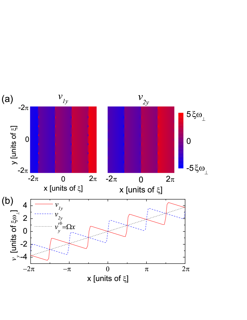
Figure 3: (Color online) (a) The tangential components $v_{1y}$ (left) and $v_{2y}$ (right) of the superfluid velocities $\mathbf{v}_{1}$ and $\mathbf{v}_{2}$ of the two states for $\Omega=0.6\omega_{\bot}$ and $T=\pi\xi$. (b) Section views of $v_{1y}$ (solid line) and $v_{2y}$ (dashed line) along the $x$ axis. The $y$ component $v_{y}^{\text{rb}}$=$\Omega x$ of the rigid body rotation velocity $\mathbf{v}^{\text{rb}}$ is shown by the dotted line for comparison.

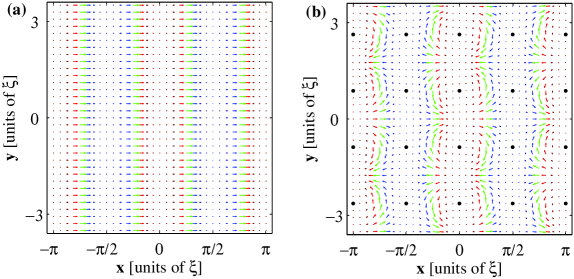
Figure 4: (Color online) The vectorial representations of the pseudospin $\mathbf{S}$ projected onto the $x$-$y$ plane for (a) $\Omega=0$, $T=\pi\xi$ and (b) $\Omega=0.6\omega_{\bot}$, $T=\pi\xi$. The colors ranging from blue to red describe the values of $S_{z}$ from $-1$ to $1$. The locations of the vortices are marked by black dots ($\bullet$).

The numerical results obtained above can be understood analytically. Considering that the $y$ component of the rigid body rotation velocity is $v_{y}^{\text{rb}}=\Omega x$, we suppose that the tangential components of the superfluid velocity on both sides of the sheet $v_{iy}^{-}$ and $v_{iy}^{+}$ are independent of $y$. According to Onsager-Feynman quantization condition single-component

$$\oint\nolimits_{\mathcal{C}}\mathbf{v}_{\text{s}}\cdot d\mathbf{l}=\frac{2\pi\hbar}{m}N_{v},$$ (3)

if we choose the two sides of the sheet as the integration path, we can obtain that the tangential velocity jump across a sheet is

$$\Delta v_{iy}=v_{iy}^{+}-v_{iy}^{-}=\frac{2\pi\hbar}{m}\frac{1}{d_{v}},$$ (4)

where $d_{v}$ is the intervortex spacing within a vortex sheet. This implies that the tangential velocity jump across the sheet is only determined by the intervortex spacing within the sheet. As the mean vortex density of each component can be estimated as

$$n_{1}=n_{2}=\frac{m\Omega}{\hbar\pi}\text{,}$$ (5)

we can obtain that the intervortex spacing within a vortex sheet is

$$d_{v}=\frac{\pi\hbar}{m\Omega T}\text{.}$$ (6)

Form Eq. (4) and Eq. (6), we have

$$\Delta v_{iy}=2\Omega T.$$ (7)

As the intersheet spacing $b$ is just equal to the period of the optical lattice potential $T$, the tangential velocity jump across the sheet can also be expressed as

$$\Delta v_{iy}=2\Omega b\text{.}$$ (8)

Meanwhile, in order to follow the rigid-body value $v_{y}^{\text{rb}}$, $v_{iy}$ must decrease $\Omega b$ in a intersheet spacing. These analytical results agree well with the numerical simulations above.

IV Domain-wall trains

The spinor order parameter of the two-component BECs allows us to analyze this system as a pseudospin-1/2 BEC and take it as a magnetic system Kasamatsu4 . Introducing a normalized complex-valued spinor $\boldsymbol{\chi}$, we represent the two-component wave functions as $\psi_{i}=\sqrt{\rho_{T}\left(\mathbf{r}\right)}\chi_{i}\left(\mathbf{r}\right)$, where $\rho_{T}\left(\mathbf{r}\right)$ is the total density and the spinor satisfies $\left|\chi_{1}\right|^{2}+\left|\chi_{2}\right|^{2}=1$. In pseudospin representation, the pseudospin density is defined as $\mathbf{S}=\boldsymbol{\chi}^{\mathbf{T}}\boldsymbol{\sigma\chi}$, where $\boldsymbol{\sigma}$ is the Pauli matrix. Then we have

$$S_{x} =2\left|\chi_{1}\right|\left|\chi_{2}\right|\cos\left(\theta_{1}-\theta_{2}\right),$$ (9)

$$S_{y} =-2\left|\chi_{1}\right|\left|\chi_{2}\right|\sin\left(\theta_{1}-\theta_{2}\right),$$ (10)

$$S_{z} =\left|\chi_{1}\right|^{2}-\left|\chi_{2}\right|^{2},$$ (11)

where $\theta_{i}$ is the phase of the wave function $\psi_{i}$.

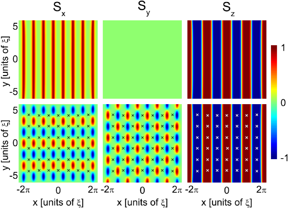
Figure 5: (Color online) The pseudospin densities $S_{x}$ (left), $S_{y}$ (middle), and $S_{z}$ (right). The upper panels show the case of $\Omega=0$ and $T=\pi\xi$, and the lower panels show the case of $\Omega=0.6\omega_{\bot}$ and $T=\pi\xi$. The locations of the vortices are marked by crosses ($\times$).

As the presence of the spin-dependent optical lattices, a train of domain walls are formed naturally at the interfaces of the two components. By the pseudospin representation, we investigate the response of the domain walls to rotation. In order to reveal the essential influence of the rotation on the structure of the domain walls, the non-rotating and rotating ground states of the two-component condensates are calculated under the same parameters. As the rotation can create an effective harmonic centrifugal potential with frequency $\Omega$ Raman , we change the radial harmonic trapping frequency to $\sqrt{\omega_{\bot}^{2}-\Omega^{2}}$ in the absence of rotation. Thus, the non-rotating ground state density distribution is nearly the same as the rotating ground state density distribution, except that no vortex is created in the low-density regions of each component in the non-rotating ground state.

The vectorial representation of the pseudospin $\mathbf{S}$ for the non-rotating and rotating ground states are presented in Figs. 4(a) and 4(b), respectively. Correspondingly, the pseudospin densities $S_{x}$, $S_{y}$ and $S_{z}$ are presented in Fig. 5. From Figs. 4 and 5, we find that a train of domain walls are formed at the interfaces of the spin up ($S_{z}=1$) and spin down ($S_{z}=-1$) regions. In the absence of rotation, the magnetic moments on the domain walls reverse only along the $x$ axis [see Fig. 4(a)], and the pseudospin density $S_{y}=0$ [see the upper panels of Fig. 5]. Therefore, these domain walls are classical Néel walls. In contrast, in the presence of rotation, the magnetic moments on the domain walls twist and form spatially periodic “eyebrow-like” spin textures [see Fig. 4(b) and the lower panels of Fig. 5]. This results in a train of novel domain walls with spatially periodic textures embedded on them.

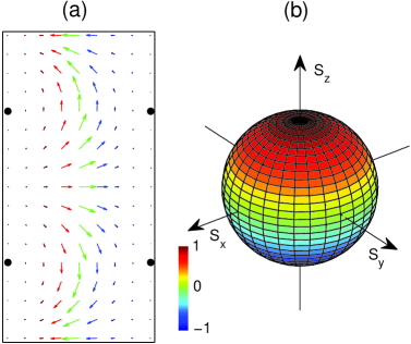
Figure 6: (Color online) (a) An amplification of Fig. 4(b) in one period. (b) Bloch sphere of the pseudospin density vector $\mathbf{S}$. Values of $S_{z}$ are represented by linear levels from blue to red ($-1$ to $1$).

It should be indicated that the classical Néel wall does not carry topological charges. However, the twist of the magnetic moments makes the novel domain wall carry topological charges. According to the topological charge density

$$q\left(\mathbf{r}\right)=\frac{1}{8\pi}\epsilon^{ij}\mathbf{S}\cdot\partial_{i}\mathbf{S}\times\partial_{j}\mathbf{S},$$ (12)

we can calculate that each period of the textures on the domain wall just carries one unit topological charge. As shown in Figs. 4 and 5, each pair of adjacent vortices from the two components just induce half texture. Since a vortex in one component is adjacent to two vortices in the other component, on average, one vortex indeed induces one half unit of topological charge. Therefore, the number of the vortices is just half the number of the topological charges.

Next, we fasten our attention on the structure of the “eyebrow-like” spin textures. An amplification of Fig. 4(b) for one period is presented in Fig. 6(a). From Eq. (9) and Eq. (10), the direction that the magnetic moments reverses along just depends on the relative phase, and can be represented by an azimuthal angle

$$\alpha=\theta_{2}-\theta_{1}\text{.}$$ (13)

From Fig. 6(a), we can see that the azimuthal angle of the magnetic moments changes from $-\pi$ to $\pi$ along the domain wall in a period, but it is constant along the normal direction of the domain wall.

It is instructive to project the pseudospin density vector $\mathbf{S}$ onto the surface of a unit Bloch sphere [see Fig. 6(b)]. Topologically, the topological charge counts the times that the Bloch sphere are covered. So one texture just covers the Bloch sphere once. From Fig. 6, we find that walking through the domain wall from one side to the other corresponds to strolling along a longitude line of the Bloch sphere from one pole to the other, and walking along the domain wall corresponds to strolling along a latitude line of the Bloch sphere. This is different from the case of a skymion, for which walking along the radial direction of the skymion corresponds to strolling along the longitude line of the Bloch sphere, and walking along the azimuthal direction of the skymion corresponds to strolling along the latitude line of the Bloch sphere. Therefore, this new texture essentially corresponds to a skyrmion in the polar coordinates instead of the Cartesian ones.

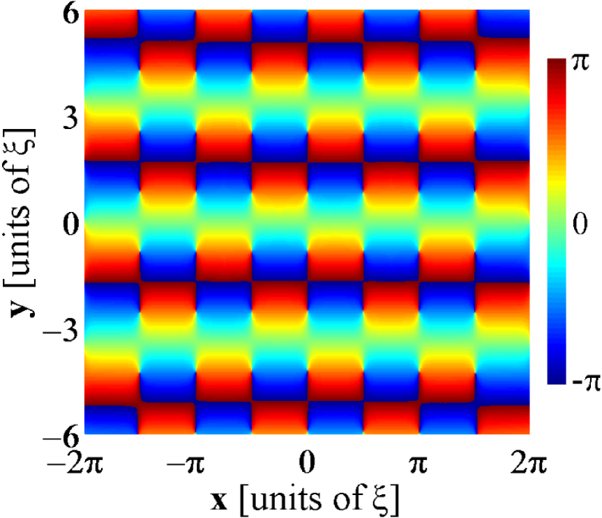
Figure 7: (Color online) The relative phase $\theta_{1}-\theta_{2}$ for $\Omega=0.6\omega_{\bot}$ and $T=\pi\xi$, where $\theta_{1}$ and $\theta_{2}$ are the phases of the wave functions $\psi_{1}$ and $\psi_{2}$, respectively.

We reveal the formation mechanism of the spatially periodic “eyebrow-like” spin textures on the domain walls. In the absence of rotation, there is no relative phase between the two components and the azimuthal angle $\alpha=0$. The magnetic moments on the domain walls only reverse along the $x$ axis. Therefore, the domain walls are classical Néel walls. In the presence of rotation, straight vortex sheets are created in the two components and arranged alternatively on two sides of the domain walls. These alternatively arranged vortex sheets induce a linear gradient of the relative phase along the domain walls [see Fig. 7]. So the azimuthal angle $\alpha$ can be expressed as

$$\alpha=\mathcal{P}\left(\kappa y\right),$$ (14)

where $\mathcal{P}$ projects the angle $\kappa y$ onto $\left(-\pi,\pi\right]$ and $\kappa$ is a constant coefficient, which describes the spatial change frequency of the azimuthal angle. The value of $\kappa$ will be given in the next section. From Eq. (14), the azimuthal angle of the magnetic moments on the domain walls changes periodically along the $y$ direction, and spatially periodic “eyebrow-like” spin textures are formed. This suggests that the spatially periodic “eyebrow-like” spin textures on the domain walls result from the linear gradient of the relative phase, which is induced by the alternating arrangement of the straight vortex sheets in the two components.

V Texture control

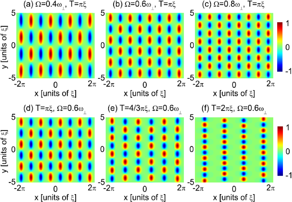
Figure 8: (Color online) The pseudospin density $S_{y}$ for different rotating angular frequencies $\Omega$ and periods of the optical lattice potential $T$. The upper panels show $S_{y}$ for $T=\pi\xi$ with (a) $\Omega=0.4\omega_{\bot}$, (b) $\Omega=0.6\omega_{\bot}$ and (c) $\Omega=0.8\omega_{\bot}$. The lower panels show $S_{y}$ for $\Omega=0.6\omega_{\bot}$ with (d) $T=\pi\xi$, (e) $T=4/3\pi\xi$ and (f) $T=2\pi\xi$.

In this section, we discuss how to control the “eyebrow-like” textures on the domain walls. Firstly, we study the distribution of the textures analytically. The topological charge density $q$ has another formulation derived from the effective velocity Mueller2

$$q\left(\mathbf{r}\right)=\frac{m}{2\pi\hbar}\left(\nabla\times\mathbf{v}_{\text{eff}}\right)_{z},$$ (15)

where the effective velocity is defined as

$$\mathbf{v}_{\text{eff}}=\frac{\left(\rho_{1}\mathbf{v}_{1}+\rho_{2}\mathbf{v}_{2}\right)}{\rho_{T}},$$ (16)

with $\rho_{i}$ the density of each component. Approximately treating the effective velocity $\mathbf{v}_{\text{eff}}$ as the classical rigid body value $\mathbf{v}_{\text{rb}}=\mathbf{\Omega}\times\mathbf{r}$, we obtain the mean topological charge density

$$\bar{q}=\frac{m\Omega}{\pi\hbar}.$$ (17)

From Eq. (17), we can calculate that the topological charge on a domain wall per unit length is

$$\eta_{q}=\frac{m\Omega T}{2\pi\hbar}.$$ (18)

This implies that the number of the textures carried by a domain wall is proportional to the rotating angular frequency $\Omega$ and the period of the optical lattice potential $T$. From Eq. (18), the spatial change frequency $\kappa$ of the azimuthal angle $\alpha$ in Eq. (14) can be calculated as

$$\kappa=2\pi\eta_{q}=\frac{m\Omega T}{\hbar}.$$ (19)

Thus, we obtain the azimuthal angle

$$\alpha=\mathcal{P}\left(\frac{m\Omega T}{\hbar}y\right).$$ (20)

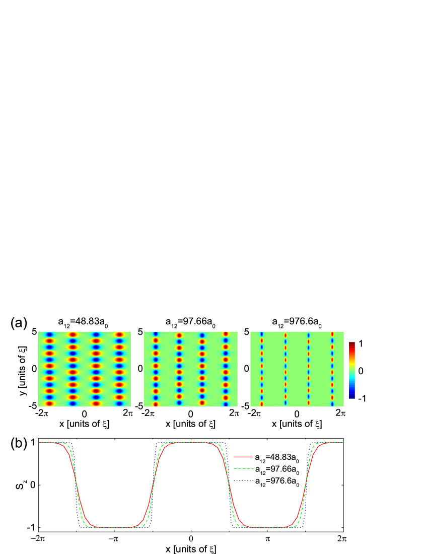
Figure 9: (Color online) (a) The pseudospin density $S_{y}$ for the intercomponent scattering length $a_{12}=48.83a_{0}$ (left), $97.66a_{0}$ (middle), and $976.6a_{0}$ (right) with the intracomponent scattering lengths $a_{11}=100.40a_{0}$ and $a_{22}=95.00a_{0}$, $\Omega=0.6\omega_{\bot}$ and $T=2\pi\xi$. (b) Cross section views of $S_{z}$ along the $x$ axis for $a_{12}=48.83a_{0}$ (solid line), $97.66a_{0}$ (dashed line), and $976.6a_{0}$ (dotted line).

In order to verify the above analytical discussion, we perform numerical simulations. The pseudospin density $S_{y}$ for different rotating angular frequencies $\Omega$ with constant period of the optical lattice potential $T$ is shown in the upper panels of Fig. 8, and $S_{y}$ for different $T$ with constant $\Omega$ is shown in the lower panels. Obviously, the number of the topological charges carried by a domain wall increases in direct proportion with the increase of $\Omega$ and $T$. For quantitative comparison, we choose $\Omega=0.6\omega_{\bot}$ and $T=\pi\xi$ as an example. From Eq. (18), we can calculate that the number of the textures on a domain wall in the region of $y=[-5\xi,5\xi]$ is $3$. This agrees well with the result of the numerical simulation in Fig. 8(b).

In our system, as the presence of the spin-dependent optical lattices, the two components are always phase separated and not subject to the immiscible condition, $g_{12}^{2}>g_{11}g_{22}$ Timmermans . However, the intercomponent interaction $g_{12}$ plays an important role on the domain wall width. As the textures are always concentrated on the walls, we can control the width of the textures by adjusting the intercomponent interaction $g_{12}$. The pseudospin densities $S_{y}$ for different intercomponent scattering length $a_{12}$ with constant intracomponent scattering lengths $a_{11}$ and $a_{22}$ are shown in Fig. 9(a). The cross section view of $S_{z}$ along the $x$ axis is shown in Fig. 9(b). From Fig. 9, we can see that with increasing the strength of intercomponent interaction, the domain walls become narrower and narrower and the textures on the walls become thinner and thinner.

VI Conclusions

We have investigated half-vortex sheets and domain-wall trains of rotating two-component BECs in spin-dependent optical lattices. A stable vortex configuration named straight half-vortex sheets is obtained. The discontinuity of the tangential component of the superfluid velocity across the sheet is discussed both numerically and analytically. We have also investigated the response of the domain walls to rotation. In the absence of rotation, the domain walls are classical Néel walls with the magnetic moments only reversing perpendicular to the walls. In response to rotation, the magnetic moments on the domain walls twist and form spatially periodic “eyebrow-like” spin textures. We have revealed that these spatially periodic textures are directly determined by the arrangement of the straight half-vortex sheets. The number of the textures carried by the domain walls can be accurately controlled by adjusting the rotating angular frequency and the period of the optical lattice, and the width of the textures can be controlled by adjusting the strength of intercomponent interaction. This allow us to make an accurate manipulation of the “eyebrow-like” textures.

With the development of the magnetization-sensitive phase-contrast imaging technique Higbie , both the longitudinal and transverse magnetization of the domain and domain wall in BECs can be imaged non-destructively with high spatial resolution Sadler ; Vengalattore . We expect that the novel domain walls with spatially periodic “eyebrow-like” spin textures would be observed in the future experiments.

References

- (1) A. L. Fetter and A. A. Svidzinsky, J. Phys. Condens. Matter 13, R135 (2001); N. R. Cooper, Adv. Phys. 57, 539 (2008); A. L. Fetter, Rev. Mod. Phys. 81, 647 (2009).
- (2) D. V. Freilich, D. M. Bianchi, A. M. Kaufman, T. K. Langin, and D. S. Hall, Science 329, 1182 (2010).
- (3) D. M. Jezek and H. M. Cataldo, Phys. Rev. A 83, 013629 (2011).
- (4) D.-S. Wang, S.-W. Song, B. Xiong, and W. M. Liu, Phys. Rev. A 84, 053607 (2011).
- (5) K. Kasamatsu, M. Tsubota, and M. Ueda, Int. J. Mod. Phys. B 19, 1835 (2005); M. Ueda and Y. Kawaguchi, e-print arXiv:1001.2072v2; M. Tsubota, K. Kasamatsu, and M. Kobayashi, e-print arXiv:1004.5458v2.
- (6) G. W. Semenoff and F. Zhou, Phys. Rev. Lett. 98, 100401 (2007).
- (7) A.-C. Ji, W. M. Liu, J. L. Song, and F. Zhou, Phys. Rev. Lett. 101, 010402 (2008).
- (8) M. Eto, K. Kasamatsu, M. Nitta, H. Takeuchi, and M. Tsubota, Phys. Rev. A 83, 063603 (2011).
- (9) S.-W. Su, C.-H. Hsueh, I.-K. Liu, T.-L. Horng, Y.-C. Tsai, S.-C. Gou, and W. M. Liu, Phys. Rev. A 84, 023601 (2011).
- (10) L. E. Sadler, J. M. Higbie, S. R. Leslie, M. Vengalattore, and D. M. Stamper-Kurn, Nature (London) 443, 312 (2006).
- (11) S. Yi and H. Pu, Phys. Rev. Lett. 97, 020401 (2006).
- (12) J. A. M. Huhtamäki, M. Takahashi, T. P. Simula, T. Mizushima, and K. Machida, Phys. Rev. A 81, 063623 (2010); J. A. M. Huhtamäki and P. Kuopanportti, Phys. Rev. A 82, 053616 (2010).
- (13) T. Kawakami, T. Mizushima, and K. Machida, Phys. Rev. A 84, 011607(R) (2011).
- (14) S.-W. Su, I.-K. Liu, Y.-C. Tsai, W. M. Liu, S.-C. Gou, e-print arXiv:1111.6338v1.
- (15) E. J. Mueller and T.-L. Ho, Phys. Rev. Lett. 88, 180403 (2002).
- (16) K. Kasamatsu, M. Tsubota, and M. Ueda, Phys. Rev. Lett. 91, 150406 (2003).
- (17) V. Schweikhard, I. Coddington, P. Engels, S. Tung, and E. A. Cornell, Phys. Rev. Lett. 93, 210403 (2004).
- (18) S. J. Woo, S. Choi, L. O. Baksmaty, and N. P. Bigelow, Phys. Rev. A 75, 031604(R) (2007).
- (19) S.-J. Yang, Q.-S. Wu, S.-N. Zhang, and S. Feng, Phys. Rev. A 77, 033621 (2008).
- (20) K. Kasamatsu and M. Tsubota, Phys. Rev. A 79, 023606 (2009).
- (21) P. Mason and A. Aftalion, Phys. Rev. A 84, 033611 (2011).
- (22) S. Coen and M. Haelterman, Phys. Rev. Lett. 87, 140401 (2001).
- (23) D. T. Son and M. A. Stephanov, Phys. Rev. A 65, 063621 (2002).
- (24) J. J. García-Ripoll and V. M. Pérez-García, Phys. Rev. A 66, 021602(R) (2002).
- (25) P. G. Kevrekidis, B. A. Malomed, D. J. Frantzeskakis, and A. R. Bishop, Phys. Rev. E 67, 036614 (2003); P. G. Kevrekidis, H. Susanto, R. Carretero-González, B. A. Malomed, and D. J. Frantzeskakis, Phys. Rev. E 72, 066604 (2005).
- (26) B. A. Malomed, H. E. Nistazakis, D. J. Frantzeskakis, and P. G. Kevrekidis, Phys. Rev. A 70, 043616 (2004); B. Deconinck, P. G. Kevrekidis, H. E. Nistazakis, and D. J. Frantzeskakis, Phys. Rev. A 70, 063605 (2004).
- (27) H. Takeuch, K. Kasamatsu, M. Nitta, and M. Tsubota, J. Low. Temp. Phys. 162, 243 (2011).
- (28) J. Jin, S. Zhang, and W. Han, J. Phys. B 44, 165302 (2011).
- (29) J.-Y. Lee, K.-S. Lee, S. Choi, K. Y. Guslienko, and S.-K. Kim, Phys. Rev. B 76, 184408 (2007); D. J. Clarke, O. A. Tretiakov, G.-W. Chern, Ya. B. Bazaliy, and O. Tchernyshyov, Phys. Rev. B 78, 134412 (2008).
- (30) O. Mandel, M. Greiner, A. Widera, T. Rom, T. W. Häsch, and I. Bloch, Phys. Rev. Lett. 91, 010407 (2003); O. Mandel, M. Greiner, A. Widera, T. Rom, T. W. Häsch, and I. Bloch, Nature (London) 425, 937 (2003).
- (31) D. McKay and B. DeMarco, New J. Phys. 12, 055013 (2010).
- (32) R. A. Battye, N. R. Cooper, and P. M. Sutcliffe, Phys. Rev. Lett. 88, 080401 (2003); H. M. Price and N. R. Cooper, Phys. Rev. A 83, 061605(R) (2011).
- (33) K. Kasamatsu, M. Tsubota, and M. Ueda, Phys. Rev. Lett. 93, 250406 (2004).
- (34) G. Ruben, M. J. Morgan, and D. M. Paganin, Phys. Rev. Lett. 105, 220402 (2010).
- (35) K. Kasamatsu, M. Tsubota, and M. Ueda, Phys. Rev. A 71, 043611 (2005).
- (36) K. M. Mertes, J. W. Merrill, R. Carretero-Gonzáez, D. J. Frantzeskakis, P. G. Kevrekidis, and D. S. Hall, Phys. Rev. Lett. 99, 190402 (2007).
- (37) K. Kasamatsu, M. Tsubota, and M. Ueda, Phys. Rev. A 67, 033610 (2003).
- (38) S. Burger, F. S. Cataliotti, C. Fort, F. Minardi, and M. Inguscio, Phys. Rev. Lett. 86, 4447 (2001).
- (39) W. Bao, I.-L. Chern, F. Y. Lim, J. Comput. Phys. 219, 836 (2006).
- (40) C. Raman, J. R. Abo-Shaeer, J. M. Vogels, K. Xu, and W. Ketterle, Phys. Rev. Lett. 87, 210402 (2001).
- (41) E. J. Mueller, Phys. Rev. A 69, 033606 (2004).
- (42) E. Timmermans, Phys. Rev. Lett. 81, 5718 (1998).
- (43) J. M. Higbie, L. E. Sadler, S. Inouye, A. P. Chikkatur, S. R. Leslie, K. L. Moore, V. Savalli, and D. M. Stamper-Kurn, Phys. Rev. Lett. 95, 050401 (2005).
- (44) M. Vengalattore, S. R. Leslie, J. Guzman, and D. M. Stamper-Kurn, Phys. Rev. Lett. 100, 170403 (2008).