Explicit construction of the pole part
of the three-gluon vertex.

Abstract:

We present an explicit construction of the special part of the three gluon vertex, which incorporates the Schwinger mechanism into the Schwinger-Dyson equation of the gluon propagator, enabling the generation of a dynamical gluon mass. This vertex contains massless, longitudinally coupled poles, acting effectively as composite Nambu-Goldstone bosons, generated by the strong QCD dynamics. The basic ingredients required for this construction are the longitudinal nature of this vertex and the Slavnov-Taylor identities that it must satisfy, in order for gauge-invariance and BRST symmetry to remain intact in the presence of a gluon mass.

1 Introduction

One of the most crucial theoretical ingredients appearing in the analysis leading to the gauge-invariant generation of an effective gluon mass [1, 2, 3, 4] is a special type of vertex, denoted by $V$, which contains massless, longitudinally coupled poles. This vertex complements the all-order three-gluon vertex entering into the Schwinger-Dyson equations (SDEs) governing the gluon self-energy, and is intimately connected with the famous Schwinger mechanism [5]. The basic underlying assumption is that the strong QCD dynamics will lead to the formation of massless bound-state excitations, which, in turn, furnish the aforementioned poles that appear inside $V$ [6, 7, 8, 9, 10].

Even though the presence of the vertex $V$ is indispensable for maintaining gauge invariance, its explicit closed form is yet undetermined [11]. This is so, in part because, at the level of the “one-loop dressed” SDE analysis carried out so far, a great deal of information on the behavior of the gluon mass may be extracted without explicit knowledge of the vertex $V$, invoking only some of its general properties, most notably the fact that it displays a completely longitudinal Lorentz structure, and that it satisfies very powerful Slavnov-Taylor identities (STIs) and Ward identities (WIs) [12].

However, in order to be able to go beyond the “one-loop dressed” approximation in the SDE studies, the closed form of $V$ is absolutely necessary. This necessity becomes particularly transparent within the formalism that has emerged from the synthesis between the pinch technique (PT) [1, 13, 14, 4, 15, 16] and the background-field method (BFM) [17], known in the literature as the PT-BFM scheme [3, 4] . In the present work we carry out the explicit construction of the vertex $V$ within this particular formalism.

2 General considerations.

In this section we introduce the appropriate notation and conventions, as well as the basic ingredients that we will use in order to construct the pole part of the three-gluon vertex as well as to motivate the necessity of determine its explicitly form. Consider then the full gluon propagator in the renormalizable $R_{\xi}$ gauges defined as

$$\Delta_{\mu\nu}(q)=-i\bigg{[}P_{\mu\nu}(q)\Delta(q^{2})+\xi\frac{q_{\mu}q_{\nu}}{q^{4}}\bigg{]},$$ (1)

where

$$P_{\mu\nu}(q)=g_{\mu\nu}-\frac{q^{\mu}q^{\nu}}{q^{2}}\,,$$ (2)

is the dimensionless transverse projector, and $\xi$ the gauge fixing parameter (a color factor $\delta^{ab}$ has been factored out). The form factor $\Delta(q^{2})$ is related to the all-order gluon self-energy $\Pi_{\mu\nu}(q)=P_{\mu\nu}(q)\Pi(q^{2})$ through

$$\Delta^{-1}(q^{2})=q^{2}+i\Pi(q^{2})=q^{2}J(q^{2}),$$ (3)

where $J(q^{2})$ is the inverse of the gluon dressing function. As a direct consequence of the gauge invariance of the theory, which after the gauge-fixing is encoded into the BRST symmetry, we know that the gluon self-energy is transverse,

$$q^{\mu}\Pi_{\mu\nu}(q)=0\,,$$ (4)

to all orders in perturbation theory, as well as non-perturbatively, at the level of the SDE.

As is well known, in the PT-BFM scheme, the SDE of the gluon propagator, shown in Fig. 1, assumes the form [3] ,

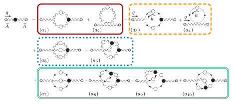
Figure 1: The SDE corresponding to the PT-BFM gluon self-energy $\Pi_{\mu\nu}$. The graphs inside each box form a gauge invariant subgroup, furnishing an individually transverse contribution. White (black) blobs denote full propagators (vertices). External background legs are indicated by the small gray circles.

$$\Delta^{-1}(q^{2})P_{\mu\nu}(q)=\frac{q^{2}P_{\mu\nu}(q)+i\Pi_{\mu\nu}(q)}{[1+G(q^{2})]^{2}}\,,$$ (5)

where the function $G(q^{2})$ is the $g_{\mu\nu}$ form factor in the Lorentz decomposition of the auxiliary function

$$\Lambda_{\mu\nu}(q) = -ig^{2}C_{A}\int_{k}D(q-k)\Delta_{\mu}^{\sigma}(k)H_{\nu\sigma}(-q,q-k,k)$$ (6)

$$= g_{\mu\nu}G(q^{2})+\frac{q_{\mu}q_{\nu}}{q^{2}}L(q^{2}),$$

where $C_{A}$ is the Casimir eigenvalue of the adjoint representation of the gauge group, and $H_{\mu\nu}$ is the standard ghost-gluon kernel, shown diagrammatically in Fig. 3, together with the dressed-loop expansion of $\Lambda_{\mu\nu}$.

One of the most powerful properties of the PT-BFM formulation is that the transversality of the gluon self-energy is realized “blockwise” [15], following the pattern shown in Fig.1.

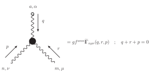
Figure 2: The BQQ vertex with the conventions for the momenta, color and Lorentz indices.

If we focus our attention on the ”one-loop dressed” gluon contributions to the PT-BFM gluon self-energy, given by the subset of diagrams $(a_{1})$ and $(a_{2})$, the relevant Green’s function to consider is the three-gluon vertex with one background leg and two quantum legs denoted by BQQ (see Fig. 2). This special vertex satisfies a WI when contracted with the momentum $q_{\alpha}$ of the background gluon leg, and two STIs when contracted with the momentum $r_{\mu}$ or $p_{\nu}$ of the quantum gluon legs [18], namely

$$q^{\alpha}\widetilde{\mathrm{I}\!\Gamma}_{\alpha\mu\nu}(q,r,p)=p^{2}J(p^{2})P_{\mu\nu}(p)-r^{2}J(r^{2})P_{\mu\nu}(r),$$

$$r^{\mu}\widetilde{\mathrm{I}\!\Gamma}_{\alpha\mu\nu}(q,r,p)=F(r^{2})\left[q^{2}\widetilde{J}(q^{2})P_{\alpha}^{\mu}(q)H_{\mu\nu}(q,r,p)-p^{2}J(p^{2})P_{\nu}^{\mu}(p)\widetilde{H}_{\mu\alpha}(p,r,q)\right],$$

$$p^{\nu}\widetilde{\mathrm{I}\!\Gamma}_{\alpha\mu\nu}(q,r,p)=F(p^{2})\left[r^{2}J(r^{2})P_{\mu}^{\nu}(r)\widetilde{H}_{\nu\alpha}(r,p,q)-q^{2}\widetilde{J}(q^{2})P_{\alpha}^{\nu}(q)H_{\nu\mu}(q,p,r)\right].$$ (7)

In these identities the ghost-gluon kernel $\widetilde{H}_{\mu\nu}$ is obtained from the conventional ${H}_{\mu\nu}$ by replacing the external gluon by a background gluon, as shown in Fig. 3. The quantity $F(q^{2})$ represents the ghost dressing function, related to the ghost propagator $D(q^{2})$ through

$$D(q^{2})=\frac{F(q^{2})}{q^{2}}.$$ (8)

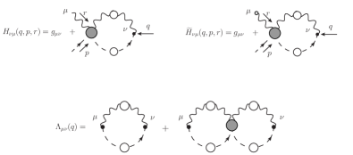
Figure 3: Diagrammatic representation of the auxiliary functions $H$, $\widetilde{H}$ and $\Lambda$. White blobs represent dressed propagators, while gray blobs denote one-particle irreducible kernels with respect to vertical cuts.

Finally, the function $\widetilde{J}(q^{2})$ corresponds to the inverse dressing function of the mixed “background-quantum” gluon propagator (one background and one quantum gluons entering, BQ), denoted by $\widetilde{\Delta}(q^{2})$. This latter propagator, together with the conventional gluon propagator (two quantum gluons entering, QQ), denoted by $\Delta(q^{2})$, and the background gluon propagator (two background gluons entering, BB), denoted by $\widehat{\Delta}(q^{2})$, are the three types of gluon propagators that appear naturally in the BFM formalism. They are related by the so called “background-quantum identities” (BQIs) [19, 20]

$$\Delta(q^{2}) = [1+G(q^{2})]^{2}\widehat{\Delta}(q^{2}),$$

$$\Delta(q^{2}) = [1+G(q^{2})]\widetilde{\Delta}(q^{2}),$$

$$\widetilde{\Delta}(q^{2}) = [1+G(q^{2})]\widehat{\Delta}(q^{2}).$$ (9)

Now, if we want to trigger the Schwinger mechanism, a pole vertex $\widetilde{V}_{\alpha\mu\nu}(q,r,p)$ containing longitudinally coupled massless bound-state excitations must be added to the conventional (fully-dressed) BQQ three-gluon vertex $\widetilde{\mathrm{I}\!\Gamma}_{\alpha\mu\nu}(q,r,p)$, giving rise to the new full vertex $\widetilde{\mathrm{I}\!\Gamma}^{\prime}_{\alpha\mu\nu}(q,r,p)$ defined as [11]

$$\widetilde{\mathrm{I}\!\Gamma}^{\prime}_{\alpha\mu\nu}(q,r,p)=\widetilde{\mathrm{I}\!\Gamma}_{\alpha\mu\nu}(q,r,p)+\widetilde{V}_{\alpha\mu\nu}(q,r,p).$$ (10)

The presence of this pole vertex enforces the gauge-invariance of the theory in the presence of masses. Specifically, when the gluon propagator becomes effectively massive, assuming the form [12, 21, 22]

$$\Delta^{-1}_{m}(q^{2})=q^{2}J(q^{2})-m^{2}(q^{2}),$$ (11)

the full vertex $\widetilde{\mathrm{I}\!\Gamma}^{\prime}$ ought to preserve the fundamental property (4); so, it must satisfy the same formal STI’s (2), but with the replacement $\Delta^{-1}\rightarrow\Delta^{-1}_{m}$. This requirement will be automatically fulfilled if we demand that the pole vertex $\widetilde{V}$ satisfies the following STI’s [11],

$$q^{\alpha}\widetilde{V}_{\alpha\mu\nu}(q,r,p)=m^{2}(r^{2})P_{\mu\nu}(r)-m^{2}(p^{2})P_{\mu\nu}(p),$$

$$r^{\mu}\widetilde{V}_{\alpha\mu\nu}(q,r,p)=F(r^{2})\left[m^{2}(p^{2})P_{\nu}^{\mu}(p)\widetilde{H}_{\mu\alpha}(p,r,q)-\widetilde{m}^{2}(q^{2})P_{\alpha}^{\mu}(q)H_{\mu\nu}(q,r,p)\right],$$

$$p^{\nu}\widetilde{V}_{\alpha\mu\nu}(q,r,p)=F(p^{2})\left[\widetilde{m}^{2}(q^{2})P_{\alpha}^{\nu}(q)H_{\nu\mu}(q,p,r)-m^{2}(r^{2})P_{\mu}^{\nu}(r)\widetilde{H}_{\nu\alpha}(r,p,q)\right].$$ (12)

The mass $\widetilde{m}$ appearing in Eq. (2) denotes the mass of the mixed background-quantum gluon propagator $\widetilde{\Delta}(q^{2})$, and it is known to satisfy the same BQI as the full gluon propagator, namely Eq.(2), i.e [12]

$$\widetilde{m}^{2}(q^{2})=[1+G(q^{2})]m^{2}(q^{2}).$$ (13)

Finally, observe that the ”two-loop dressed” gluon contribution to the PT-BFM gluon self-energy, given by the subset of diagrams $(a_{5})$ and $(a_{6})$ in Fig. 1, contains an internal three-gluon vertex with three quantum gluon legs (QQQ), as well as a four-gluon vertex with one background and three quantum gluon legs (BQQQ). This BQQQ vertex satisfies the following WI when contracted with respect to the background gluon leg [15],

$$q_{1}^{\mu}\widetilde{\mathrm{I}\!\Gamma}^{abcd}_{\mu\nu\alpha\beta}(q_{1},q_{2},q_{3},q_{4}) = igf^{abx}\mathrm{I}\!\Gamma^{cdx}_{\alpha\beta\nu}(q_{3},q_{4},q_{1}+q_{2})$$ (14)

$$+ igf^{acx}\mathrm{I}\!\Gamma^{dbx}_{\beta\nu\alpha}(q_{4},q_{2},q_{1}+q_{3})$$

$$+ igf^{adx}\mathrm{I}\!\Gamma^{bcx}_{\nu\alpha\beta}(q_{2},q_{3},q_{1}+q_{4}).$$

Therefore, the description of the ”two-loop dressed” gluon block in the presence of vertices with pole structures requires the knowledge of the pole QQQ three-gluon vertex, denoted by $V$. In this case, the background leg $q_{\alpha}$ becomes quantum, and the Abelian-like WI in (2) is replaced by an STI, namely

$$q^{\alpha}V_{\alpha\mu\nu}(q,r,p)=F(q^{2})\left[m^{2}(r^{2})P^{\alpha}_{\mu}(r)H_{\alpha\nu}(r,q,p)-m^{2}(p^{2})P^{\alpha}_{\nu}(p)H_{\alpha\mu}(p,q,r)\right],$$ (15)

while the STIs with respect to the other two legs are those of Eq. (2), but with the “tilded” quantities replaced by conventional ones.

3 Explicit construction.

Turns out the the explicit closed form of the two pole vertices in question, $\widetilde{V}$ and $V$, may be determined from the STIs they satisfy, and the requirement of complete longitudinality, i.e, condition [11]

$$P^{\alpha\beta}(q)P^{\mu\rho}(r)P^{\nu\sigma}(p)\widetilde{V}_{\beta\rho\sigma}(q,r,p)=0.$$ (16)

Specifically, opening up transverse projectors in (16), one can write the entire vertex in terms of its own divergences,

$$\widetilde{V}_{\alpha\mu\nu}(q,r,p) = \frac{q_{\alpha}}{q^{2}}q^{\beta}\widetilde{V}_{\beta\mu\nu}+\frac{r_{\mu}}{r^{2}}r^{\rho}\widetilde{V}_{\alpha\rho\nu}+\frac{p_{\nu}}{p^{2}}p^{\sigma}\widetilde{V}_{\alpha\mu\sigma}-\frac{q_{\alpha}r_{\mu}}{q^{2}r^{2}}q^{\beta}r^{\rho}\widetilde{V}_{\beta\rho\nu}-\frac{q_{\alpha}p_{\nu}}{q^{2}p^{2}}q^{\beta}p^{\sigma}\widetilde{V}_{\beta\mu\sigma}$$ (17)

$$- \frac{r_{\mu}p_{\nu}}{r^{2}p^{2}}r^{\rho}p^{\sigma}\widetilde{V}_{\alpha\rho\sigma}+\frac{q_{\alpha}r_{\mu}p_{\nu}}{q^{2}r^{2}p^{2}}q^{\beta}r^{\rho}p^{\sigma}\widetilde{V}_{\beta\rho\sigma}.$$

Note that the last term will not contribute because if we apply the STI’s,

$$q^{\beta}r^{\rho}p^{\sigma}\widetilde{V}_{\beta\rho\sigma}(q,r,p)=0.$$ (18)

So, using (2) to evaluate the various terms, and after a straightforward rearrangement, we obtain the following expression for the pole part of the BQQ vertex,

$$\widetilde{V}_{\alpha\mu\nu}(q,r,p) = \frac{q_{\alpha}}{q^{2}}\left[m^{2}(r^{2})-m^{2}(p^{2})\right]P_{\mu}^{\rho}(r)P_{\rho\nu}(p)$$ (19)

$$+ D(r^{2})\left[m^{2}(p^{2})P_{\nu}^{\rho}(p)\widetilde{H}_{\rho\alpha}(p,r,q)-\widetilde{m}^{2}(q^{2})P_{\alpha}^{\rho}(q)P_{\nu}^{\sigma}(p)H_{\rho\sigma}(q,r,p)\right]r_{\mu}$$

$$+ D(p^{2})\left[\widetilde{m}^{2}(q^{2})P_{\alpha}^{\rho}(q)H_{\rho\mu}(q,p,r)-m^{2}(r^{2})P_{\mu}^{\rho}(r)\widetilde{H}_{\rho\alpha}(r,p,q)\right]p_{\nu}.$$

Applying the same procedure but using now the STIs (15) as well as the longitudinally coupled condition (16), we derive the closed expression for the pole part of the QQQ vertex

$$V_{\alpha\mu\nu}(q,r,p) = D(q^{2})\left[m^{2}(r^{2})H_{\rho\sigma}(r,q,p)-m^{2}(p^{2})H_{\sigma\rho}(p,q,r)\right]P_{\mu}^{\rho}(r)P_{\nu}^{\sigma}(p)q_{\alpha}$$ (20)

$$+ D(r^{2})\left[m^{2}(p^{2})P^{\rho}_{\nu}(p)H_{\rho\alpha}(p,r,q)-m^{2}(q^{2})P_{\alpha}^{\rho}(q)P_{\nu}^{\sigma}(p)H_{\rho\sigma}(q,r,p)\right]r_{\mu}$$

$$+ D(p^{2})\left[m^{2}(q^{2})P^{\rho}_{\alpha}(q)H_{\rho\mu}(q,p,r)-m^{2}(r^{2})P_{\mu}^{\rho}(r)H_{\rho\alpha}(r,p,q)\right]p_{\nu}.$$

Now we need to discuss some points related to the self-consistency of our vertex construction. Observe that in order to obtain expressions (19) and (20) one must apply sequentially the WI and the STIs. In doing so, the Bose symmetry of both vertices is no longer explicit, and the result obtained is not manifestly symmetric under the quantum gluon legs exchange. Furthermore, seemingly different expressions are obtained, depending on which of the two momenta acts first on $\widetilde{V}$. However, if one imposes the simple requirement of algebraic commutativity between the WI and the STIs satisfied by the three-gluon vertex, the Bose symmetry becomes manifest. For example, using (19) we can see that the elementary requirement

$$q^{\alpha}r^{\mu}\widetilde{V}_{\alpha\mu\nu}(q,r,p)=r^{\mu}q^{\alpha}\widetilde{V}_{\alpha\mu\nu}(q,r,p)\,,$$ (21)

gives rise to the following identity

$$F(r^{2})P_{\nu}^{\mu}(p)q^{\alpha}\widetilde{H}_{\mu\alpha}(p,r,q)=-r_{\mu}P_{\nu}^{\mu}(p).$$ (22)

A similar identity is obtained by imposing the requirement of (21) at the level of $V$, namely

$$F(r^{2})P_{\nu}^{\mu}(p)q^{\alpha}H_{\mu\alpha}(p,r,q)=-F(q^{2})P_{\nu}^{\mu}(p)r^{\alpha}H_{\mu\alpha}(p,q,r).$$ (23)

Quite remarkably, the identities (22) and (23) are a direct consequence of WI and the STI that the kernels $H$ and $\widetilde{H}$ satisfy, when they are contracted with the momentum of the background or quantum gluon leg, namely [18],

$$q^{\alpha}\widetilde{H}_{\mu\alpha}(p,r,q)=-p_{\mu}F^{-1}(p^{2})-r_{\mu}F^{-1}(r^{2}),$$

$$q^{\alpha}H_{\mu\alpha}(p,r,q)=-F(q^{2})\left[p_{\mu}F^{-1}(p^{2})C(q,r,p)+r^{\alpha}F^{-1}(r^{2})H_{\mu\alpha}(p,q,r)\right],$$ (24)

where $C(q,r,p)$ is the auxiliary function that characterizes the four-ghost kernel (see Fig. 4). Indeed, use of (3) into (22) and (23), respectively, leads to a trivial identity.

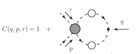
Figure 4: Diagrammatic representation of the auxiliary function $C(q,p,r)$.

Conversely, one may actually derive (3) from (22) and (23); for example, starting with (22), and using also the identities [18]

$$p^{\mu}\widetilde{H}_{\mu\alpha}(p,r,q) = r_{\alpha}F^{-1}(r^{2})-\widetilde{\Gamma}_{\alpha}(r,q,p),$$

$$q^{\alpha}\widetilde{\Gamma}_{\alpha}(r,q,p) = p^{2}F^{-1}(p^{2})-r^{2}F^{-1}(r^{2}),$$ (25)

one can easily reproduce (3)

Evidently, these constraints allow us to cast the pole part of the BQQ vertex into a manifestly Bose symmetric form with respect to the quantum legs,

$$\widetilde{V}_{\alpha\mu\nu}(q,r,p)=\frac{q_{\alpha}}{q^{2}}\left[m^{2}(r^{2})-m^{2}(p^{2})\right]P_{\mu}^{\rho}(r)P_{\rho\nu}(p)+\widetilde{I}_{\alpha\mu\nu}(q,r,p)-\widetilde{I}_{\alpha\nu\mu}(q,p,r),$$ (26)

with

$$\widetilde{I}_{\alpha\mu\nu}(q,r,p) = D(r^{2})m^{2}(p^{2})P_{\nu}^{\rho}(p)\widetilde{H}_{\rho\alpha}(p,r,q)r_{\mu}$$ (27)

$$- \frac{r_{\mu}}{2}D(r^{2})\widetilde{m}^{2}(q^{2})P_{\alpha}^{\rho}(q)\left[g_{\nu}^{\sigma}+P_{\nu}^{\sigma}(p)\right]H_{\rho\sigma}(q,r,p).$$

Finally, for the pole part of the QQQ vertex, the Bose symmetric expression reads

$$V_{\alpha\mu\nu}(q,r,p)=I_{\alpha\mu\nu}(q,r,p)-I_{\mu\alpha\nu}(r,q,p)-I_{\alpha\nu\mu}(q,p,r),$$ (28)

with

$$I_{\alpha\mu\nu}(q,r,p) = \frac{q_{\alpha}}{2}D(q^{2})\left[m^{2}(r^{2})P_{\mu}^{\rho}(r)H_{\rho\nu}(r,q,p)-m^{2}(p^{2})P_{\nu}^{\rho}(p)H_{\rho\mu}(p,q,r)\right]$$ (29)

$$+ \frac{q_{\alpha}}{2}D(q^{2})\left[m^{2}(r^{2})H_{\rho\sigma}(r,q,p)-m^{2}(p^{2})H_{\sigma\rho}(p,q,r)\right]P_{\mu}^{\rho}(r)P_{\nu}^{\sigma}(p).$$

4 Conclusions.

In this work we have reported the explicit closed form of the pole parts of two particular vertices, which are intimately connected to the phenomenon of gluon mass generation, as described within the PT-BFM formalism. Specifically, we have determined the pole parts of the BQQ and QQQ vertices, denoted by ${\tilde{V}}$ and $V$, respectively. The only ingredient necessary for this construction is the longitudinal nature of ${\tilde{V}}$ and $V$ and the STIs and WIs that they must satisfy. These two vertices are expected to form an integral part of the ongoing SDE studies that aim to determine the precise quantitative details of the gluon mass generation mechanism.

References

[1]
J. M. Cornwall,
Phys. Rev. D 26, 1453 (1982).
[2]
C. W. Bernard,
Phys. Lett. B108, 431 (1982);
Nucl. Phys. B219, 341 (1983).
[3]
A. C. Aguilar, D. Binosi and J. Papavassiliou,
Phys. Rev. D 78, 025010 (2008).
[4]
D. Binosi and J. Papavassiliou,
Phys. Rept. 479, 1-152 (2009).
[5]
J. S. Schwinger,
Phys. Rev. 125, 397 (1962);
Phys. Rev. 128, 2425 (1962).
[6]
R. Jackiw and K. Johnson,
Phys. Rev. D 8, 2386 (1973).
[7]
R. Jackiw,
In *Erice 1973, Proceedings, Laws Of Hadronic Matter*, New York 1975, 225-251 and M I T Cambridge - COO-3069-190 (73,REC.AUG 74) 23p.
[8]
J. M. Cornwall and R. E. Norton,
Phys. Rev. D 8 3338 (1973).
[9]
E. Eichten and F. Feinberg,
Phys. Rev. D 10, 3254 (1974).
[10]
E. C. Poggio, E. Tomboulis and S. H. Tye,
Phys. Rev. D 11, 2839 (1975)).
[11]
A. C. Aguilar, D. Ibanez, V. Mathieu and J. Papavassiliou,
arXiv:1110.2633 [hep-ph].
[12]
A. C. Aguilar, D. Binosi and J. Papavassiliou,
Phys. Rev. D 84, 085026 (2011).
[13]
J. M. Cornwall and J. Papavassiliou,
Phys. Rev. D 40, 3474 (1989).
[14]
A. Pilaftsis,
Nucl. Phys. B 487, 467 (1997).
[15]
A. C. Aguilar and J. Papavassiliou,
JHEP 0612, 012 (2006).
[16]
D. Binosi and J. Papavassiliou,
Phys. Rev. D 77(R), 061702 (2008);
JHEP 0811, 063 (2008).
[17]
See, e.g., L. F. Abbott,
Nucl. Phys. B 185, 189 (1981), and references therein.
[18]
D. Binosi and J. Papavassiliou,
JHEP 1103, 121 (2011).
[19]
P. A. Grassi, T. Hurth and M. Steinhauser,
Annals Phys. 288 (2001) 197.
[20]
D. Binosi and J. Papavassiliou,
Phys. Rev. D 66 (2002) 025024.
[21]
A. Cucchieri and T. Mendes,
PoS LAT2007, 297 (2007).
[22]
O. Oliveira, P. J. Silva,
Phys. Rev. D79, 031501 (2009);
PoS LAT2009, 226 (2009).