Confinement in G(2) Gauge Theories Using Thick Center Vortex Model and domain structures

Abstract

The thick center vortex model with the idea of using domain structures is used to calculate the potentials between two G($2$) heavy sources in the fundamental, the adjoint and the $27$ dimensional representations. The potentials are screened at large distances. This behavior is expected from the thick center vortex model since G($2$) has only a trivial center element which makes no contribution to the average Wilson loop at the large distance regime. A linear potential is obtained at intermediate distances for all representations. This behavior can be explained by the thickness of the vortices (domains) and by defining a flux for the trivial center element of G($2$). The role of the SU($3$) subgroup of G($2$) in the linear regime is also discussed. The string tensions are in rough agreement with the Casimir operators of the corresponding representations.

PACS. 11.15.Ha, 12.38.Aw, 12.38.Lg, 12.39.Pn

I INTRODUCTION

The last candidate for the fundamental theory of hadronic force is the quark model. The interaction between quarks is described by the exchange of the non-Abelian gauge fields called gluons. Quarks were introduced by Gellman and Zweig for the first time in 1964. Besides the successfulness of the quark model, no free quark has been observed yet. However, the particles in the Lagrangian of any theory must exist in the physical spectrum. Now that the quarks appear in the QCD Lagrangian, the main question is as follows: Where are the quarks? Are they permanently confined? In fact, these are not the quarks which are not found in the nature but it is the color which is confined and quarks are confined because of their colors. In other words, particles with color degrees of freedom are confined. Therefore, all free particles are colorless, and colored particles cannot be found in the particle spectrum. Also gluons, particles in the adjoint representation of the gauge group of QCD have colors, and are absent in the particle spectrum, as well.

Let us define confinement from the point of view of the potential in a quark-antiquark pair. At short distances the potential in a quark-antiquark pair is Coulombic and can be explained by the gluon exchange between quarks. Since the coupling constant is small, perturbative methods work very well in this region. As the distances between quarks increase, the coupling constant increases as well and perturbative techniques do not work anymore. This happens at an intermediate regime where the potential between quarks rises linearly until the energy reaches a point where it is large enough to create a quark-antiquark pair in the vacuum. Then, these secondary pairs couple to the initial ones and screen them. However, by removing the dynamical quarks from the theory, the creation of the secondary quarks does not happen and the potential between the initial quarks rises linearly with distance. Figure (1) shows a typical behavior of the potential between static quark s, a Coulombic potential at short distances, and a linear potential for intermediate and large distances. For this figure, dynamical quarks are removed from the theory. The linear behavior is confirmed by Regge trajectories in the particle spectrum Collins1968 . The flux tube created at this linear regime has nonlinear nature, and it is not possible to use ordinary perturbation methods to study its characteristics. Therefore, to investigate the quark confinement phenomena, one should use nonperturbative methods. Lattice gauge theory has been very successful to reproduce the potential between pairs of colored particles like quarks and gluons. Other approaches used to study confinement include phenomenological models. In these models, the QCD vacuum is filled with some topological configurations confining colored objects. The most popular candidates among these topological fields are monopoles and vortices. Other candidates include merons, calorons,$\it{etc}$. There are very strong correlations between these various objects, though. Therefore, the mechanism of confinement has not been understood by a unique procedure yet, and it is one of the unsolved mysteries of quantum chromodynamics.

In this paper, we study the center vortex model within the G(2) gauge group. The center vortex model was initially introduced by ’t Hooft Hooft1979 . It was able to explain the confinement of quark pairs, but it was not able to explain the intermediate linear potential,especially for higher representations.The model has been improved to the thick center vortex model by M. Faber $\it{et~{}al.}$ Fabe1998 . Even though it is a simple model, the thick center vortex model reproduces the intermediate linear potential qualitatively, in agreement with Casimir scaling and the asymptotic large distance potential which is proportional to the $N$-ality of the gauge group. For intermediate distances, one expects to see a linear potential proportional to the distance between quarks, in agreement with lattice calculations. Based on lattice results Bali2000 ; Deld1999 , the coefficient of the linear part which is called the string tension, is proportional to the eigenvalue of t he quadratic Casimir operator of the corresponding representation. This is called Casimir scaling. The Casimir scaling regime is expected to extend roughly from the onset of confinement to the onset of screening. The $N$-ality of each representation is given by mod($n-m$), where $n$ is the number of quarks and $m$ is the number of antiquarks constructing the representation. At large distances, where the distance between the quark and antiquark increases, the energy stored in the string increases and gluon pairs are created from the vacuum. These gluons screen the initial sources to the lowest dimension with the same $N$-ality. In this regime, sources with the same $N$-ality obtain the same string tensions. Those with zero $N$-ality are completely screened.

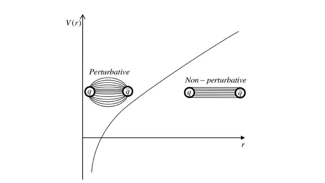
Figure 1: Potential between static quarks. At small distances the coupling constant is small enough to use perturbative methods. A Coulombic potential is obtained in this regime. At large distances the coupling constant is large, and nonperturbative effects lead to a linear potential.

In the vortex model the QCD vacuum is filled with linelike (in three dimensions) or surfacelike (in four dimensions) objects, which carry magnetic flux quantized in terms of the center elements of the gauge group. At large distances between color sources, the interactions between Wilson loops and center vortices lead to a linear potential proportional to the $N$-ality of the given representation.

Besides the successes of the center vortex model, the relation between confinement and center symmetry has not been understood very well,yet. To study the role of center elements, one of the attractive methods is studying confinement in gauge groups without nontrivial center elements, like G($2$). Lattice calculations in G($2$) Olejnik2008 show color screening for large distances and a linear potential for intermediate distances. Since the center is trivial, the center vortex model predicts color screening. It is not so clear why a linear potential can be expected at intermediate distances. Because of these two features confinement at intermediate distances and screening at large distances G(2) gauge theory resembles SU($N$) gauge theories with dynamical quarks. These screen static quarks at large distances. Therefore, G($2$) is considered as a mathematical laboratory to examine the properties of SU($N$) gauge theories, even the ones which can not be understood in SU($N$) gauge theories themselves.

In the next section, we give a brief review of the thin and thick center vortex models. In Sec.III, some general features of the G(2) gauge group are discussed, and in Sec.IV we apply the improved thick center vortex model, called the domain structure model, to the G($2$) gauge group. We study the possible reasons why confinement is observed in the G($2$) gauge group based on its SU(3) subgroups. Potentials between static sources of higher representations, $14$ and $27$, are calculated in Sec.V, and Casimir scaling is discussed. We end the paper with a conclusion.

II Thick Center Vortex Model

The idea of describing confinement using vortices goes back to ’t Hooft Hooft1979 . In four dimensions vortices are topological field configurations of the vacuum forming closed surfaces which can be linked to Wilson loops. Wilson loops are gauge-invariant observables obtained from the holonomy of the gauge connection around given loops. Confinement is obtained from random fluctuations in the linking number. A vortex piercing a Wilson loop contributes with a center element $Z$ somewhere between the group elements $U$ of the gauge group

$$W(C)=\mathrm{Tr}[UUU\ldots U]\longrightarrow\mathrm{Tr}[UUU\ldots(Z)\ldots U].$$ (1)

Because center elements commute with all the members of the group, the location of $Z$ in Eq.(1) is arbitrary. The effect of piercings on Wilson loops can be well understood in the gauge group SU($2$), which has $-I$ as the only nontrivial center element. $I$ is the $2\times 2$ unit matrix. Vortices piercing the loop an even number of times or not piercing it at all, do not have any effect on $W(C)$. Odd linking numbers change the sign of $W(C)$. One can derive a formula for the string tension $\sigma$ assuming that vortices are thin and pierce Wilson loops in single plaquettes with independent probabilities $f$. We get

$$\langle W(C)\rangle=\prod\{(1-f)+f(-1)\}\langle W_{0}(C)\rangle=\exp[-\sigma(c)A]\langle W_{0}(C)\rangle$$ (2)

assuming that $\langle W_{0}(C)\rangle$ is the expectation value of the loop when no vortex pierces this loop and the string tension is

$$\sigma=-\frac{1}{A}\ln(1-2f).$$ (3)

The vortex model works very well for the fundamental representation, and it gives the asymptotic string tension correctly. It also works well for the adjoint representation at large distances, where one expects a screened potential. Since we have a trivial center element for the adjoint representation, the string tension must be zero according to Eq.(1). In other words, $Z$ is unity and it does not change the Wilson loop. However, lattice calculations show an intermediate string tension for higher representations Higher ; Deld1999 ; Bali2000 , which can not be predicted by the thin center vortex model or Eq.(1). M. Faber $\it{et~{}al.}$ Fabe1998 have improved the model to the thick center vortex model to be able to reproduce the intermediate string tensions. They have given a thickness to the ’t Hooft vortex. Mathematically, they have replaced the center element $Z$ by an element of the gauge group, $G$,

$$W(C)=\mathrm{Tr}[UUU\ldots U]\longrightarrow\mathrm{Tr}[UUU\ldots G\ldots U]$$ (4)

where G is

$$G(x,s)=\exp(i\alpha_{c}(x)\overrightarrow{n}\cdot\overrightarrow{L}).$$ (5)

$L_{i}$’s are the generators of the group in the representation $j$, $\overrightarrow{n}$ is a unit vector, and $S$ is an SU($N$) element of the group in the representation $j$. $\alpha_{c}(x)$ gives the profile of the vortex, and it depends on that fraction of the vortex which is pierced by the loop. It depends on the shape of the loop $C$ and the position of the center of the vortex relative to the perimeter of the loop.

If the Wilson loop is linked by $m$ vortices, centered at positions $x_{1},x_{2},...,x_{m}$, then

$$W(C)\longrightarrow W[C;\{x_{i},S_{i}\}]=\mathrm{Tr}[UUU\ldots UG\{x_{a},S_{a}\}U\ldots\\ UG\{x_{b},S_{b}\}U\ldots UG\{x_{m},S_{m}\}U].$$ (6)

To obtain the average Wilson loop, $W(C)$ must be averaged over different gauge group orientations $S_{i}$. For simplicity, we first look at the SU($2$) case. Equation (5) for SU($2$) is

$$G(x,s)=\exp(i\alpha_{c}(x)\overrightarrow{n}\cdot\overrightarrow{L})=S\exp(i\alpha_{c}(x)L_{3})S^{\dagger}.$$ (7)

$L_{3}$ is the element of the Cartan subalgebra.Independently averaging every $G\{x_{a},S_{a}\}$ over orientations in the group manifold specified by $S_{a}$, we get

$$\bar{G}(a)=\int\!S\exp[i\alpha L_{3}]S^{\dagger}\,\mathrm{d}S=g_{j}[\alpha_{c}]I_{2j+1}$$ (8)

where

$$g_{j}[\alpha_{c}]=\frac{1}{2j+1}\mathrm{Tr}(\exp[i\alpha L_{3}]).$$ (9)

Thus, averaging the Wilson loop over all $S_{a}$ leads to Fabe1998

$$\langle W(C)\rangle=\prod_{x}\{(1-f)+fg_{j}[\alpha_{c}]\}\langle W_{0}(C)\rangle$$ (10)

$$=\exp[\sum_{x}\ln\{(1-f)+fg_{j}[\alpha_{c}]\}]\langle W_{0}(C)\rangle$$ (11)

$$=\exp[-\sigma_{c}A]\langle W_{0}(C)\rangle$$ (12)

where $\sigma_{c}$ is

$$\sigma_{c}=\frac{-1}{A}\sum_{x}\ln\{(1-f)+fg_{j}[\alpha_{c}]\}.$$ (13)

For large loops, the center element is located completely inside the loop; thus $g_{j}[\alpha_{c}]=-1$, and the string tension is

$$\sigma_{c}=-\frac{1}{A}\ln(1-f-f)=-\ln(1-2f).$$ (14)

This string tension is the same for all half integer representations $j$. For integer representations for which a flat potential is expected at large distances, the center element is trivial and $g_{j}[\alpha_{c}]=1$; thus $\sigma_{c}=0$ according to Eq.(13).

At intermediate distances where the loop is not large enough to contain the whole vortex, $\sigma_{c}$ is Fabe1998

$$\sigma_{c}=\frac{f}{6}\bar{\alpha}_{c}^{2}j(j+1)$$ (15)

where

$$\bar{\alpha}_{c}^{2}=\frac{1}{A}\sum_{x\in A^{\prime}}\alpha_{c}^{2}(x).$$ (16)

Thus, for small $f$ and small loops, the string tension is proportional to the eigenvalue of the second order Casimir operator.

Equation (10) can be generalized to the SU($N$) gauge theory

$$\langle W(C)\rangle=\prod_{x}{(1-\sum_{n=1}^{N}f_{n}(1-g_{r}[\vec{\alpha}_{c}^{n}(x)]))}\langle W_{0}(C)\rangle$$ (17)

with

$$g_{r}[\vec{\alpha}]=\frac{1}{d_{r}}\mathrm{Tr}(\exp[i\vec{\alpha}\cdot\vec{H}]).$$ (18)

$x$ is the location of the center of the vortex, $d_{r}$ the dimension of the representation $r$, $f_{n}$ the probability that any given unit is pierced by a vortex of type $n$, and $\{H_{i},i=1,2,...,N-1\}$ are the generators spanning the Cartan subalgebra. $\vec{\alpha}_{c}^{n}(x)$ shows the flux profile for the vortex of type $n$. We have $(N-1)$ types of vortices for any SU($N$) gauge theory. The potential and the string tension are given by Fabe1998

$$V(R)=\sum_{x}\ln\left\{1-\sum^{N-1}_{n=1}f_{n}(1-{\mathrm{Re}}g_{r}[\vec{\alpha}^{n}_{C}(x)])\right\}$$ (19)

and

$$\sigma_{C}=-\frac{1}{A}\sum_{x}\ln[{1-\sum_{n=1}^{N-1}f_{n}(1-{\mathrm{Re}}g_{r}[\vec{\alpha}_{C}^{n}(x)])}].$$ (20)

To reproduce the potential or the string tension, one has to find the Cartan subalgebra and describe the profile function $\vec{\alpha}_{C}^{n}(x)$. The flux profile should have the following properties: It should go to zero for a Wilson loop of length $R$ as $x\rightarrow\pm\infty$; if the center of a vortex is completely inside the loop, it will lead to a maximal multiplicative factor $\exp({\frac{2\pi in}{N}})\in Z_{n}$ $(n=1,2,...,N-1)$ corresponding to the center elements of the group; and finally as $R\rightarrow 0$ the contribution of the vortex to the loop also goes to zero , so $\alpha_{R}(x)\rightarrow 0$.

Various vortex profiles $\vec{\alpha}_{C}^{n}(x)$ may be chosen. M. Faber $\it{et~{}al.}$ used, for the SU($2$) case,

$$\vec{\alpha}_{C}^{n}(x)=\vec{N}^{n}[1-\tanh(ay(x)+\frac{b}{R})]$$ (21)

where $n$ indicates the vortex type, $a,b$ are arbitrary constants, and $y(x)$ is

$$y(x)=\begin{cases}-x&\lvert R-x\lvert>x\\ x-R&\lvert R-x\lvert\leqslant x\end{cases}$$ (22)

$y(x)$ is the nearest distance of $x$ from the timelike side of the loop. The normalization constant $\vec{N}^{n}$ is obtained from the maximum flux condition, where the loop contains the vortex completely,

$$\exp(i\vec{\alpha}^{n}\cdot\vec{H})=z_{n}I$$ (23)

with

$$z_{n}=e^{\frac{2\pi in}{N}}\in Z_{N}$$ (24)

and $I$ is the unit matrix.

The thick center vortex model has worked well for the SU($2$), SU($3$), and SU($4$) gauge theories Fabe1998 , Deld . A linear potential in rough agreement with Casimir scaling is observed for all representations, and the asymptotic string tension proportional to the $N$-ality of the given representation has been reported. To increase the length of the linear regime at intermediate distances, J. Greensite $\it{et~{}al.}$ Green2007 have suggested postulating a kind of domain structure in the vacuum, with magnetic flux in each domain quantized in units corresponding to the elements of the center subgroup, including the identity element. They have applied this idea to the SU($2$) gauge group which has one trivial and one nontrivial center element. Thus, instead of one vortex, they use two kinds of domain structures corresponding to the center elements, the trivial and nontrivial elements. To obtain the Wilson loop, Eq. (10) should be changed to

$$\langle W(C)\rangle=\prod_{x}\{(1-f_{1}-f_{0})+f_{0}g_{j}[\alpha_{C}^{0}]+f_{1}g_{j}[\alpha_{C}^{1}]\}\langle W_{0}(C)\rangle.$$ (25)

$f_{1}$ and $f_{0}$ are the probabilities of plaquettes that belong to domains corresponding to the nontrivial and trivial center elements, respectively. $\alpha_{C}^{0}$ and $\alpha_{C}^{1}$ define the profile function for domain structures associated with the trivial and nontrivial center elements. To apply the domain structure model to the SU($N$) gauge group, one has to change $n$ in Eqs. (17), (19) and (20) from zero to the number of nontrivial center elements, where zero corresponds to the trivial center element.

G($2$) lattice gauge calculations show confinement for intermediate distances Olejnik2008 . The center vortex model can predict correctly the screening of the potentials at large distances since the center of the G($2$) gauge group is trivial. But, what accounts for the intermediate string tensions? We apply the domain structure model, which includes the trivial center element, to the G($2$) gauge group in Sec.IV and discuss the possible reasons for the linear potential at large distances. But first, in Sec.III, we present some general features of the gauge group G($2$).

III General properties of G($2$) gauge theories

G($2$) is one of the exceptional Lie groups which is its own covering group Pepe . The rank of G($2$) is 2 and it has 14 generators,two of which are simultaneously diagonal. Its fundamental representation is seven dimensional, and the dimension of the adjoint representation is 14. The group G($2$) is real, and it is a subgroup of SO($7$) with rank 3 and 21 generators. The determinant of the $7\times 7$ real orthogonal matrices $U$ of the group SO($7$) is $1$, and

$$UU^{\dagger}=1.$$ (26)

G($2$) elements satisfy a constraint called the cubic constraint,

$$T_{abc}=T_{def}U_{da}U_{eb}U_{fc}$$ (27)

$T$ is a totally antisymmetric tensor, and its nonzero elements are

$$T_{127}=T_{154}=T_{163}=T_{235}=T_{264}=T_{374}=T_{576}=1.$$ (28)

Because of these constraints the number of generators of G($2$) is reduced to $14$.

A quark in the fundamental representation $\{7\}$ of G($2$) can be color screened by gluons Pepe ,

$$\{7\}\otimes\{14\}\otimes\{14\}\otimes\{14\}=\{1\}\oplus...$$ (29)

Therefore, in G($2$) gauge theories, the string tension between static quarks can be broken by gluons without the presence of dynamical quarks, as is necessary in SU($N$) gauge theories.

SU($3$) is a subgroup of G($2$). Under SU(3) subgroup transformations, the seven and $14$-dimensional representations of G($2$) decompose into the SU($3$) fundamental and adjoint representations

$$\{7\}=\{3\}\oplus\{\overline{3}\}\oplus\{1\},$$ (30)

$$\{14\}=\{8\}\oplus\{3\}\oplus\{\overline{3}\}.$$ (31)

The second equation may be interpreted in such a way that the $14$ gluons of G($2$) consist of the usual eight gluons of SU($3$) plus six additional gluons which transform like the SU($3$) fundamental quark and antiquark. One of the differences between these six gluons and the SU($3$) quarks is that the former are bosons while the latter are fermions. Because all G($2$) representations are real, the fundamental representation is equivalent to its complex conjugate; therefore quarks and antiquarks are identical.

Simultaneous diagonal generators of this representation are Pepe

$$H^{3}=\frac{1}{\sqrt{8}}(P_{11}-P_{22}-P_{55}+P_{66}),$$ (32)

$$H^{8}=\frac{1}{\sqrt{24}}(P_{11}+P_{22}-2P_{33}-P_{55}-P_{66}+2P_{77})$$ (33)

where $(P_{ij})_{\alpha\beta}=\delta_{i\alpha}\delta_{j\beta}$ , and $\alpha,\beta$ indicate the row and the column of the matrices, respectively. From Eqs. (32) and (33), it can be shown that these generators have SU($3$) Cartan generators, and they can be written as

$$H^{a}=\frac{1}{\sqrt{2}}\left(\begin{array}[]{ccc}\lambda^{a}&0&0\\ 0&\;0&0\\ 0&0&-(\lambda^{a})^{*}\end{array}\right).$$ (34)

$\lambda^{a}$ ($a=3,8$) are the two diagonal SU(3) generators. Since SU($3$) is a subgroup of the G($2$) gauge group, the G($2$) weight diagram can be obtained by a superposition of $3$, $1$, and $\bar{3}$. Therefore, in the SU($3$) subgroup of G($2$), the center elements of G($2$) can be constructed from Z($3$), the center of SU($3$)

$$Z=\left(\begin{array}[]{ccc}zI_{3\times 3}&0&0\\ 0&1&0\\ 0&0&z^{*}I_{3\times 3}\end{array}\right).$$ (35)

$I_{3\times 3}$ is a $3\times 3$ unit matrix and $z\in\{1,e^{\pm\frac{2\pi i}{3}}\}$ are elements of $Z(3)$. The three Z matrices of Eq.(35) commute with the eight generators of the SU($3$) subgroup of G($2$) but not with the remaining six generators. This is why the centers Z given by Eq. (35) are not the center elements of G($2$). The center elements should commute with all the generators. Therefore, the center of G($2$) should be trivial and contains only the identity. This is true for higher representations of G($2$) as well. Since the center element of G($2$) is trivial for all representations, at large distances the potentials between objects in all representations are flat and screening happens. Equation (29) shows this fact for the seven dimensional representation. Another consequence is that the concept of $N$-ality does not apply to the G($2$) gauge group, in contrast to the SU($N$) gauge groups.

In the next section, we calculate the potential between two G($2$) quarks using the domain structure model.

IV G($2$) and vacuum domain structures

Numerical calculations Olejnik2008 show a linear behavior at intermediate distances and a flat potential at large distances for the potential between two quarks in the fundamental and higher representations of the G($2$) gauge theory. Even though G($2$) does not have any nontrivial center element, its trivial center element can explain the flat potential according to the thick center vortex model. Based on this model no vortex means no string tension at large distances, and this is in agreement with the flat potential for the G($2$) quarks at large distances. In this section we reproduce the potential in a G($2$) quark antiquark pair using the idea of domain structures of the vacuum in the thick center vortex model.

Greensite $\it{et~{}al.}$ have introduced domain structures to increase the length of the linear regime in the thick center vortex model Green2007 . They have suggested that the domain structure idea can be applied to the G($2$) gauge group which has only a trivial center. With this motivation, we apply the idea to calculate the G($2$) potentials explicitly. In SU($N$), zero $N$-ality representations have zero string tensions at large distances, while they have linear potentials at intermediate distances. The thick center vortex model has been able to reproduce this behavior, and we have been motivated to use this model to reproduce G($2$) potentials which show the same behavior according to the lattice results but with the idea of domain structures instead of center vortices. Thickening the vortices leads to the confinement for higher SU($N$) representations. Since G($2$) has only a trivial center element, we apply the thick center vortex model to this group with the constraint that the total magnetic flux measured by the Wilson loop holonomy is quantized in terms of its trivial center element.

In the domain structure model, the vacuum of the Yang-Mills theory is filled with field configurations called domain structures, corresponding to trivial and nontrivial center elements. For example, for SU($2$)there exist two type of domains, one associated with the trivial one, $I$, and one associated with the nontrivial one, $-I$. The main difference between the trivial domain and other domains is the lack of a Dirac-3 volume for trivial domains.

Equation (19) can be used in the SU($N$) gauge group for the modified thick center vortex model, if $n$ starts from zero instead of 1, where $n=0$ corresponds to the trivial center element. For the G($2$) case with only a trivial center element and no other nontrivial center elements, $V(R)$ is given by

$$V(R)=\sum_{x}\ln\left\{1-f_{0}(1-{\mathrm{Re}}g_{r}[\vec{\alpha}^{0}_{C}(x)])\right\}.$$ (36)

where $f_{0}$ is the probability that any given unit is pierced by a trivial vacuum domain. $g_{r}$ has the same form as in Eq. (18),

$$g_{r}[\vec{\alpha}]=\frac{1}{d_{r}}\mathrm{Tr}(\exp[i\vec{\alpha}\cdot\vec{H}]).$$ (37)

We use the flux profile

$$\alpha_{i}^{0}(x)=N_{i}^{0}[1-\tanh(ay(x)+\frac{b}{R})].$$ (38)

The zero index indicates the trivial domain of G($2$), and the index $i$ is the index of the Cartan generators. $a$ and $b$ are free parameters of the model. The normalization factor is obtained by using the maximum flux condition of Eq. (23). For G($2$), the equation is changed to

$$\exp(i\vec{\alpha}^{n}\cdot\vec{H})=I.$$ (39)

Therefore,

$$\exp(\alpha_{1}^{max}H_{1}+\alpha_{2}^{max}H_{2})=I=\exp(2\pi i).$$ (40)

Using the Cartan subalgebra of G($2$) from Eq. (34), $\alpha_{1}^{max}$ and $\alpha_{2}^{max}$ are obtained,

$$\begin{array}[]{c}2\pi=\frac{\alpha_{1}^{max}}{\sqrt{8}}+\frac{\alpha_{2}^{max}}{\sqrt{24}}\\ 2\pi=\frac{-\alpha_{1}^{max}}{\sqrt{8}}+\frac{\alpha_{2}^{max}}{\sqrt{24}}\end{array}\}\Longrightarrow~{}~{}\alpha_{1}^{max}=0,~{}~{}\alpha_{2}^{max}=2\pi\sqrt{24}.$$ (41)

Thus, $\alpha_{1}^{0}(x)$ and $\alpha_{2}^{0}(x)$ are

$$\alpha_{1}^{0}(x)=0,$$ (42)

$$\alpha_{2}^{0}(x)=\frac{\pi}{\sqrt{24}}[1-\tanh(ay(x)+\frac{b}{R})].$$ (43)

Putting everything together, the potential between two G($2$) static quarks is obtained from Eqs. (36) to (38) and is plotted in Fig. (2). The free parameters $a$, $b$, and $f$ are chosen to be $0.05$, $4$, and $0.1$, respectively. The potential is screened at large distances as expected from the model. At large distances the domains are contained completely inside the loops, and the corresponding contribution, which is the trivial center element, does not change the Wilson loop; therefore, the string tension is zero. At intermediate distances a linear regime is observed. For this regime, some fraction of the trivial domain is located inside the loop. Therefore it can make a nontrivial contribution to the Wilson loop and lead to a nonzero string tension.

Figure 2: Potentials between two G($2$) static quarks obtained from the domain structure model. The potential is screened at large distances, in agreement with the fact that the gluons of the G($2$) gauge group can couple to the quarks in the fundamental representation and give a singlet. A linear potential is observed for the intermediate distances.

Figure 3: ${\mathrm{Re}}(g_{r}[\alpha^{0}_{2}(x)])$ versus $x$ is plotted for the fundamental representation of the G($2$) gauge group. It varies between $1$ and $-0.28$. The value of $1$ indicates the situation where the Wilson loop either does not link the vortex or it links the vortex completely. ${\mathrm{Re}}(g_{r}[\alpha^{0}_{2}(x)])=-0.28$ can be explained by the SU($3$) subgroup of G($2$) as explained in the text.

Figure 4: The same as Fig. (3) but for $R=20$. The minimum of ${\mathrm{Re}}(g_{r}[\alpha^{0}_{2}(x)])$ reaches $-0.28$ for this intermediate $R$ as well.

To study the possible reasons for the linear part, we plot ${\mathrm{Re}}(g_{r}[\alpha^{0}_{2}(x)])$ versus $x$ for the Wilson loop, with various spatial dimensions of $R$. Figure (3) plots ${\mathrm{Re}}(g_{r}[\alpha_{2}^{0}(x)])$ versus $x$ for $R=100$. $x$ shows the location of the center of the vortex. The left leg of the Wilson loop is located at zero, and the right leg is located at $x=R$. The maximum of ${\mathrm{Re}}(g_{r})$ is equal to 1 and indicates either the situation where the domain does not link to the Wilson loop or the one where it is located completely inside the loop. For the profile we are using, the size of the domain is proportional to the inverse of the parameter $a$, and it is about $20$. Therefore, when the Wilson loop spatial length is equal to $100$, we are sure that a complete link is established between the Wilson loop and the vortex. This fact is observed from the figure, since ${\mathrm{Re}}(g_{r})$ reaches $1$ when the center of the vortex is located at $x\approx 50$.

${\mathrm{Re}}(g_{r})$ reaches a value of 1 when the vortex is completely inside a Wilson loop. In SU($N$) the result would be different, and a non-trivial center element is obtained. Another interesting feature of the figure is the minimum of ${\mathrm{Re}}(g_{r})$ which is around $-0.28$. In general, for the SU($N$) cases ${\mathrm{Re}}(g_{r})$ varies from $1$, corresponding to the trivial center element, to the values corresponding to the nontrivial center elements. Since G($2$) does not have any nontrivial center element, predicting the amount of the lower limit is not clear. The minimum of ${\mathrm{Re}}(g_{r})$, can be interpreted using the SU(3) subgroup of G($2$). SU($3$) has three center elements (domains): $e^{\frac{n\pi i}{3}}$, where $n$ changes from zero to 2. ${\mathrm{Re}}(g_{r}[\alpha^{0}_{2}(x)])$, corresponding to these center elements, varies between $1$ and $-0.5$ since

$$e^{\frac{2\pi i}{3}}=-0.5+\frac{\sqrt{3}}{2}i.$$ (44)

Now, calculating ${\mathrm{Re}}(g_{r}[\alpha^{0}_{2}(x)])$ of the G($2$) gauge group using its SU($3$) subgroup and normalizing it with the dimension of the subgroup, we get the minimum of ${\mathrm{Re}}(g_{r}[\alpha^{0}_{2}(x)])$,

$${\mathrm{Re}}g_{r}([\alpha^{0}_{2}(x)])_{\mathrm{min}}=\frac{1}{7}(\mathrm{Tr}(e^{i\alpha\cdot H})_{\mathrm{min}})=\frac{1}{7}\mathrm{Tr}\left(\begin{array}[]{ccc}{\acute{g_{R}}(\alpha)_{\mathrm{min}}\times d_{r}}&0&0\\ 0&1&0\\ 0&0&{\acute{g_{R}}(\alpha)_{\mathrm{min}}\times d_{r}}\end{array}\right).$$ (45)

where ${\acute{g_{R}}}(\alpha)_{\mathrm{min}}$ is the minimum of ${\mathrm{Re}}(g_{r})$ for the SU($3$) subgroup, and it is equal to $-0.5$ as mentioned above. $d_{r}$ is the dimension of the subalgebra which is equal to 3. Thus, the minimum of ${\mathrm{Re}}(g_{r})$ for the group G($2$) is obtained as

$${\mathrm{Re}}(g_{r})_{\mathrm{min}}=\frac{1}{7}(\mathrm{Tr}(e^{i\alpha\cdot H})_{\mathrm{min}})=\frac{1}{7}(-1.5+1-1.5)=-0.28.$$ (46)

Some other local minimums are observed for ${\mathrm{Re}}(g_{r})$ in Fig. (3) which may be interpreted by the SU($2$) subgroups of G($2$). Reaching the minimum of $-0.28$ happens for the intermediate distances $R$ as well. Figure (4) shows ${\mathrm{Re}}(g_{r}[\alpha^{0}_{2}(x)])$ for $R=20$.

Going back to Fig.(2), because of the trivial center of the G($2$) gauge group, at large distances a screened potential is expected from thin or thick center vortex models. However, the linear regime is observed as a result of using thick vortices, as seen for the SU($N$) higher representations with zero N-ality. On the other hand, studying the flux profile, ${\mathrm{Re}}(g_{r}[\alpha^{0}_{2}(x)])$, the role of the SU($3$) subgroup of G($2$) must be considered as another possible reason to interpret the linear behavior. One may claim that, at intermediate distances, the SU($3$) subgroup of G($2$) has a dominant role, and this fact leads to the observation of a linear potential at this regime.

Pepe $\it{et~{}al.}$ Pepe have studied the role of the SU($3$) subgroup with a Higgs mechanism. They have exploited a scalar Higgs field in representation $7$ of G($2$), which breaks G($2$) to SU($3$). This allows for interpolation between theories with exceptional confinement like G($2$) and theories with ordinary confinement like SU($3$). An interpretation of G($2$) confinement via its SU($3$) subgroup and using the domain structure model needs more investigation, and the present paper may be considered as one of the starting points.

In the next section, we find the potentials between heavy sources for the higher representations $14$ and $27$, and we discuss Casimir scaling of the string tension.

V Potentials between static G($2$) sources of higher representations

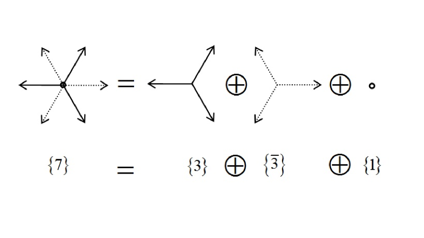
Figure 5: Weight diagram of the fundamental representation of G($2$) decomposed into its SU($3$) subgroups.

Sources with dimensions $14$ and $27$ are obtained by

$$\{7\}\otimes\{7\}=\{1\}\oplus\{7\}\oplus\{14\}\oplus\{27\}.$$ (47)

To calculate the potentials with the domain structure model, one has to use Eqs. (36) and (37). As Eq. (37) demands, $H$, the Cartan subalgebra of G($2$) must be calculated for the $14$- and $27$- dimensional representations. We use the weight diagrams of the SU($3$) gauge group, and we decompose each representation of the G($2$) gauge group to its SU($3$) subgroups to obtain the weight diagrams for G($2$) representations. It is clear from Eq. (34) that the weight diagram of the G($2$) fundamental representation can be obtained by Fig. (5). This is because the fundamental representation of G($2$) can be decomposed into its SU($3$) subgroup representations

$$\{7\}=\{3\}\oplus\{\bar{3}\}\oplus\{1\}$$ (48)

where $3$ and $\bar{3}$ show the fundamental representations of the SU($3$) group.

For the adjoint representation of G($2$) with dimension $14$, the decomposition is as follows:

$$\{14\}=\{3\}\oplus\{\bar{3}\}\oplus\{8\}.$$ (49)

The $8$ indicates the adjoint representation of SU($3$). Thus, the Cartan subalgebra of the adjoint representation can be calculated from the weight diagrams of Fig. (6) and Eq. (49),

$$H_{14}=\frac{1}{\sqrt{8}}\left(\begin{array}[]{ccc}\lambda_{3}&0&0\\ 0&\;-{\lambda_{\bar{3}}}^{*}&0\\ 0&0&\lambda_{8}\end{array}\right).$$ (50)

where $\lambda_{3}$, $\lambda_{\bar{3}}$, and $\lambda_{8}$ are the Cartan subgroups of SU($3$) for the representations $3$, ${\bar{3}}$, and $8$, respectively.

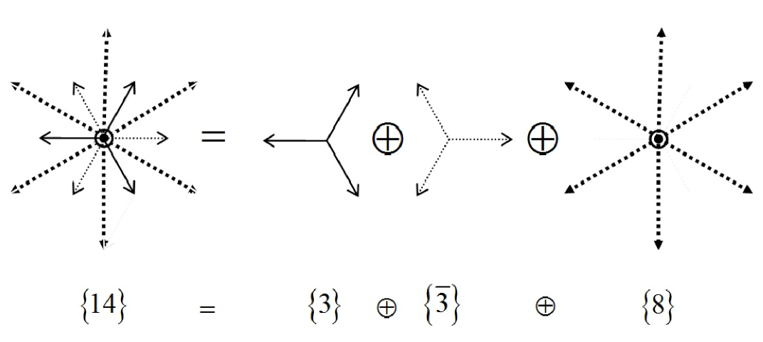
Figure 6: Weight diagram of the adjoint ($14$-dimensional) representation of G($2$) decomposed into its SU($3$) subgroups.

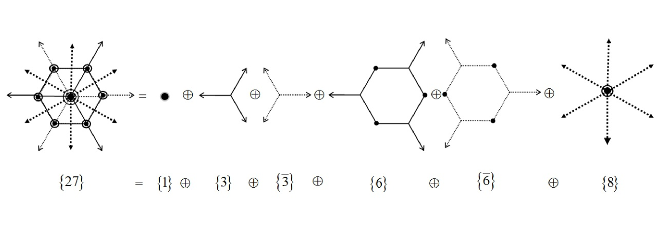
Figure 7: Weight diagram of the representation $27$ of G($2$) decomposed into its SU($3$) subgroups.

Representation $27$ of the G($2$) gauge group is obtained from Eq. (47). But like the fundamental and adjoint representations of G($2$), the weight diagram of representation $27$ can be obtained by decomposition to its SU($3$) subgroups. Figure (7) shows this decomposition, where $6$ and $\bar{6}$ are the six dimensional representations of SU($3$). In fact,

$$\{27\}=\{8\}\oplus\{6\}\oplus\{\bar{6}\}\oplus\{3\}\oplus\{\bar{3}\}\oplus\{1\}.$$ (51)

Therefore, the Cartan subalgebra of representation $27$ is

$$H_{27}=\frac{1}{\sqrt{18}}\left(\begin{array}[]{cccccc}\lambda_{8}&0&0&0&0&0\\ 0&\lambda_{6}&0&0&0&0\\ 0&0&-{\lambda_{\bar{6}}}^{*}&0&0&0\\ 0&0&0&\lambda_{3}&0&0\\ 0&0&0&0&-{\lambda_{\bar{3}}}^{*}&0\\ 0&0&0&0&0&0\end{array}\right).$$ (52)

We recall that for all representations of G($2$) we use the normalization condition

$$\mathrm{Tr}[T_{a}T_{b}]=\frac{1}{2}\delta_{ab}.$$ (53)

Figure 8: Potentials between two G($2$) static sources in the fundamental, $14$ and $27$ dimensional representations. The potentials are screened at large distances in agreement with the fact that gluons of the G($2$) gauge group can couple to the initial sources and a singlet is produced. For each representation, a linear potential is observed at intermediate distances.

Figure 9: Potentials between two G($2$) static sources in the fundamental, $14$ and $27$ dimensional representations at intermediate distances. The ratio of the string tension of each representation to the string tension of the fundamental representation is qualitatively in rough agreement with the Casimir ratio.

The next step is to find the normalization factors in Eq. (38) for these two new representations. We use Eq. (39), with $\vec{H}$ the Cartan subgroups of representations $14$ and $27$. For both representations $\alpha_{1}^{max}=0$ and $\alpha_{2}^{max}$ is equal to $\pi\sqrt{24}$ for the adjoint and $6\pi\sqrt{24}$ for the $27$ representation . Now, we are ready to calculate the potentials from Eq. (36) with the profile function of Eq. (38). Fig. (8) plots the potentials for the fundamental, adjoint, and $27$ representations. The free parameters $a$, $b$, and $f$ are chosen to be $0.05$, $4$, and $0.1$, respectively. The potentials are screened at large distances, as expected from the fact that G($2$) has only a trivial center. In fact, the representations $14$ and $27$ lead to a singlet after they combine with gluons that popped out of the vacuum. This happens when the distance between static sources is large enough and the potential between sources is big enough to create a pair of heavy gluons.

$$\{7\}\otimes\{14\}\otimes\{14\}\otimes\{14\}=\{1\}\oplus...$$ (54)

$$\{14\}\otimes\{14\}=\{1\}\oplus...$$ (55)

$$\{27\}\otimes\{14\}=\{7\}\oplus\{14\}\oplus\{27\}\oplus...$$ (56)

One of the interesting points of the figure is that the sources in the fundamental representation are screened at higher energy than the adjoint sources. This can be explained by the above equations which indicate that a fundamental quark interacting with three gluons leads to a singlet, while adjoint sources are screened by interacting with one gluon. Therefore, screening happens at higher energies for the fundamental representation compared to the adjoint representation. The sources of the $27$-dimensional representation do not give a singlet after combining with a pair of gluons. Screening happens if the adjoint sources produced from Eq. (56) interact with the adjoint sources again and a singlet is produced according to Eq. (55).

It is observed from Fig.(8) that the potentials are concave at intermediate distances. It is worse for representation $14$. To get a nonconcave potential and to be able to calculate the string tensions more accurately, we use the method of Ref. Rafi which considers some random fluctuations for the vortex profiles. Figure (9) shows the potentials at intermediate distances. A linear regime is observed for all three representations. However, the length of this area is very small. The Casimir scaling regime is expected to extend roughly from the onset of confinement to the onset of screening. String tensions are calculated for $R$ between $5$ and $12$. From Fig. (9), the string tension ratios are

$$\frac{K_{14}}{K_{f}}=1.48,~{}~{}~{}~{}~{}~{}~{}~{}~{}~{}~{}~{}~{}~{}~{}~{}~{}~{}~{}~{}~{}~{}~{}\frac{K_{27}}{K_{f}}=1.65,$$ (57)

while the Casimir ratios are

$$\frac{C_{14}}{C_{f}}=2,~{}~{}~{}~{}~{}~{}~{}~{}~{}~{}~{}~{}~{}~{}~{}~{}~{}~{}~{}~{}~{}~{}~{}\frac{C_{27}}{C_{f}}=\frac{7}{3}.$$ (58)

The string tension ratios are qualitatively in rough agreement with Casimir ratios. The agreement between Casimir ratios and string tension ratios obtained from the lattice calculations is very good Olejnik2008 . However, we recall that the thick center vortex model predictions for proportionality with Casimir scaling for SU($2$), SU($3$), and SU($4$) have also been very rough Fabe1998 ; Deld . The Casimir ratios of representations $27$ to $14$ is $1.16$, which is in good agreement with the string tension ratios obtained from the model, about $1.12$, in Eq. (57). It is also possible to find the potentials between static sources in other higher representations of the G($2$) gauge group, but finding the Cartan subalgebra from the weight diagrams would be a little bit harder. However, studying these three representations of the G($2$) gauge group shows that the thick center vortex model, with the idea of the domain structure, works rather w ell even in the G($2$) gauge group which has only a trivial center.

VI conclusion

Studying confinement in gauge groups without nontrivial center elements is an attractive subject. G($2$) is one of these exceptional groups which has only a trivial center. Lattice calculations show some evidence for the confinement of quarks at intermediate distances. On the other hand, the thick center vortex model is a phenomenological model which gives potentials between quarks in gauge groups with nontrivial center elements. In this paper, to reproduce the lattice results, the idea of the vacuum domain structure has been used in the thick center vortex model. A flux has been assigned to the trivial center of the G($2$), gauge group and the potential between two static G($2$) quarks is obtained. The potential is screened at large distances, as expected from the thick center vortex model. In other words, the trivial center does not affect the Wilson loop, where a complete link is established between them at large distances. In this regime, the vortex (domain) is located completely inside the minimal area of the loop. A linear potential at intermediate distances is observed. The thickness of the domains and possibly the SU($3$) subgroups of the G($2$) gauge group are responsible for this linear behavior at intermediate distances.

In addition, potentials between static sources of the adjoint and the $27$ -dimensional representations are calculated by the model. In both cases, the potentials are linear at intermediate distances, and the string tensions are qualitatively in rough agreement with Casimir scaling.

VII Acknowledgments

We would like to thank Manfried Faber and Stefan Olejnik for very helpful discussions. We are grateful to the research council of the University of Tehran for supporting this study.

References

- (1) P. D. Collins, E. J. Squires, Regge poles in particle physics, 1968, Springer, New York.
- (2) G. ’t Hooft, Nucl. Phys. B 138, 1978, p. 1; G. Mack, in Recent development in gauge Theories, edited by G. ’t Hooft et al. (Plenum, New York, 1980); H. B. Nielson, P. Olesen, Nucl. Phys. B 160, p. 380, 1979; J. Ambjørn, P. Olesen, Nucl. Phys. B 170, p. 60 and p. 265, 1980; J. Cornwall, Nucl. Phys. B 157, p. 392, 1979; R. Feynman, Nucl. Phys. B 188, p. 479, 1981.
- (3) M. Faber, J. Greensite, S. Olejnik, Phys. Rev. D 57, p. 2603, 1998.
- (4) G. S. Bali, Casimir scaling of SU(3) static potentials, Phys. Rev. D 62, p. 114503, 2000.
- (5) S. Deldar, Phys. Rev. D 62, p. 034509, 2000.
- (6) L. Liptak, S. Olejnik, Phys. Rev. D 78, p. 074501, 2008; Bjorn H. Wellegehausen, A. Wipf, C. Wozar, Phys. Rev. D 83, p. 016001, 2011; Bjorn H. Wellegehausen, A. Wipf, C. Wozar, Phys. Rev. D 83, p. 114502, 2011.
- (7) C. Bernard, Phys. Lett. B 108, p. 431; Nucl. Phys. B 219, p. 341, 1983; J. Ambjørn, P. Olesen, C. Peterson, Nucl. Phys. B 240, p. 189, 1984; C. Michael, Nucl. Phys. B 259, p. 58, 1985; G. Poulis, H. Trottier, Phys. Lett. B 400, p. 358, 1997.
- (8) S. Deldar, JHEP 0101, p. 013, 2001, S. Deldar, S. Rafibakhsh, Phys. Rev. D 76, p. 094508, 2007.
- (9) J. Greensite, K. Langfeld, S. Olejnik, H. Reinhardt, T. Tok, Phys. Rev. D 75, p. 034501, 2007.
- (10) K. Holland, P. Minkowski, M. Pepe, U. J. Wiese, Nucl. Phys. B 668, p. 207, 2003, M. Pepe, U. J. Wiese, Nucl. Phys. B 768, p. 21, 2007; Bjorn H. Wellegehausen, A. Wipf, C. Wozar, Phys. Rev. D 83, p. 016001, 2011.
- (11) S. Deldar, S. Rafibakhsh, Phys. Rev. D 81, p. 054501, 2010.