Dislocation core field. II. Screw dislocation in iron

Abstract

The dislocation core field, which comes in addition to the Volterra elastic field, is studied for the $\langle 111\rangle$ screw dislocation in alpha-iron. This core field, evidenced and characterized using ab initio calculations, corresponds to a biaxial dilatation, which we modeled within the anisotropic linear elasticity. We show that this core field needs to be considered when extracting quantitative information from atomistic simulations, such as dislocation core energies. Finally, we look at how dislocation properties are modified by this core field, by studying the interaction between two dislocations composing a dipole, as well as the interaction of a screw dislocation with a carbon atom.

I Introduction

Ab initio calculations have revealed that a $\langle 111\rangle$ screw dislocation in $\alpha$-iron creates a core field in addition to the Volterra elastic field Clouet et al. (2009). This core field corresponds to a pure dilatation in the $\left\{111\right\}$ plane perpendicular to the dislocation line. It is responsible for a non negligible volume change per unit length of dislocation line. The core field decays more rapidly than the Volterra field, as the displacement created by this core field varies as the inverse of the distance to the dislocation line, whereas the displacement caused by the Volterra field varies as the logarithm of this distance. Such a dislocation core field is not specific to iron: a similar dilatation induced by the core of the screw dislocation can be deduced from the analysis of core structures obtained from first-principles in other body-centered cubic (bcc) metals, such as Mo and Ta Ismail-Beigi and Arias (2000); Frederiksen and Jacobsen (2003). Atomistic simulations in other crystal structures have also led to such a core field Gehlen et al. (1972); Hoagland et al. (1976); Woo and Puls (1977); Henager and Hoagland (2004, 2005).

The purpose of this paper is to characterize this core field for a $\langle 111\rangle$ screw dislocation in iron, and to see how it modifies the dislocation properties. In that purpose, ab initio calculations have been used to obtain the dislocation core structure. Then the dislocation core field has been modeled within the linear anisotropic elasticity theory, using the approach initially developed by Hirth and Lothe Hirth and Lothe (1973), and generalized in the preceding paper Clouet (2011) to incorporate the core field contribution into the dislocation elastic energy. This modeling allows extracting quantitative information from ab initio calculations, such as the dislocation core energy. Finally, the effect of the core field on the interaction of a screw dislocation with a carbon atom has been investigated, as well as on the properties of a screw dislocation dipole.

II Atomistic simulations

II.1 Dislocation dipole

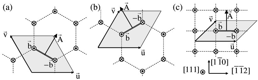
Figure 1: Screw dislocation periodic arrangements used for ab initio calculations: (a) T and (b) AT triangular arrangements, (c) quadrupolar arrangement. $\mathbf{u}$ and $\mathbf{v}$ are the unit cell periodicity vectors, and $\mathbf{A}$ the dipole cut vector. In all cases, the Burgers vector $\mathbf{b}=\frac{1}{2}a_{0}\left[111\right]$ for easy, and $-\frac{1}{2}a_{0}\left[111\right]$ for hard core configuration.

Fully periodic boundary conditions have been selected to study the $\langle 111\rangle$ screw dislocation in $\alpha$-Fe. A dislocation dipole is introduced into the simulation box, using three different periodic distributions of dislocations. Within the triangular arrangement, initially proposed by Frederiksen and Jacobsen Frederiksen and Jacobsen (2003), the dislocations are positioned on a honeycomb network [Figs. 1(a) and 1(b)] that strictly preserves the threefold symmetry of the bcc lattice along the $\left[111\right]$ direction. Two different variants, which are linked by a $\pi/3$ rotation, are possible for this periodic arrangement: the twinning (T) [Fig. 1(a)] and the anti-twinning (AT) [Fig. 1(b)] triangular arrangement. The name of the variant refers to the fact that the dislocation dipole has been created by shearing a $\left\{112\right\}$ plane either in the T or AT orientation. The third periodic arrangement, represented in Fig. 1(c), is equivalent to a rectangular array of quadrupoles. The periodicity vectors $\mathbf{u}$ and $\mathbf{v}$ defining these different arrangements are given in Ref. Ventelon and Willaime, 2007. For all periodic arrangements, the periodicity vector along the dislocation line is taken as the minimal allowed vector, i.e. the Burgers vector $b=\frac{1}{2}a_{0}\left[111\right]$ where $a_{0}$ is the lattice parameter. Thus the number of atoms in the simulation box is directly proportional to the surface $S$ of the unit cell perpendicular to the dislocation line.

For each periodic arrangement, the dislocations are positioned at the center of gravity of three neighboring $\left[111\right]$ atomic columns. Depending on the sign of the Burgers vector, two types of cores can be obtained Vitek (1974). In the easy core configuration, the helicity of the lattice is locally reversed compared to the helicity of the perfect lattice. This configuration has been found to be the most stable in all atomistic simulations in bcc transition metals. In the hard core configuration, the three central neighboring $\left[111\right]$ atomic columns are shifted locally so that these atoms lie in the same $\left(111\right)$ plane. This configuration actually corresponds to a local maximum of the energy of the dislocation arrangement. It can be nevertheless stabilized numerically by symmetry in the atomistic simulations. The three periodic arrangements sketched in Fig. 1 allow us to simulate a dipole whose both dislocations are either in their easy or hard core configurationVentelon and Willaime (2007).

The dislocation dipole is introduced into the simulation cell by applying the displacement field of each dislocation, as given by the anisotropic linear elasticity. A homogeneous strain is also applied to the periodicity vectors, to minimize the elastic energy contained within the simulation box Lehto and Öberg (1998); Cai et al. (2001, 2003); Li et al. (2004); Clouet et al. (2009). This homogeneous strain corresponds to the plastic strain produced when the dislocation dipole is introduced into the simulation unit cell. It is given by

$$\varepsilon_{ij}^{0}=-\frac{b_{i}A_{j}+b_{j}A_{i}}{2S}.$$

The orientations of the Burgers vector, $\mathbf{b}$, and of the dipole cut vector, $\mathbf{A}$, are defined in Fig. 1. Then the atomic positions are relaxed so as to minimize the energy of the simulation box computed by ab initio calculations Ventelon and Willaime (2007).

Two types of simulations have been performed in this work: simulations at constant volume and at zero stress. One can keep the periodicity vectors fixed and minimize the energy only with respect to the atomic positions. Within this constant volume simulation, the simulation box is subject to a homogeneous stress. Within the zero stress simulation, the unit cell is allowed to relax its size and shape, so that the homogeneous stress vanishes at the end of the relaxation. In both cases, the dislocation core field can be identified.

II.2 Ab initio calculations

The present ab initio calculations in bcc iron have been performed in the density functional theory (DFT) framework using the Siesta codeSoler et al. (2002), i.e. the pseudopotential approximation and localized basis sets, as in Refs. Fu et al., 2004 and Ventelon and Willaime, 2007. Comparison with plane-waves DFT calculations Ventelon and Willaime (2010) has shown that this Siesta approach is reliable to study dislocations in bcc iron. The charge density is represented on a real space grid with a grid spacing of $0.06$ Å that has been reduced after self-consistency to $0.03$ Å. The Hermite-Gaussian smearing technique with a $0.3$ eV width has been used for electronic density of state broadening. These calculations are spin-polarized and eight valence electrons are considered for iron. The Perdew-Burke-Ernzerhof (PBE) generalized gradient approximation (GGA) scheme is used for exchange and correlation. A $3\times 3\times 16$ $k$-point grid is used for the dislocation calculations with unit cells containing up to 361 atoms, and a $16\times 16\times 16$ grid for the elastic constants.

The obtained Fe lattice parameter is $a_{0}=2.88$ Å, in good agreement with the experimental value (2.85 Å). The DFT elastic constants are deduced from a fit on a fourth order polynomial over the energies for different strains ranging from $-2$ to $2$ %. This leads to the values of $248$, $146$ and $69$ GPa for the elastic constants $C_{11}$, $C_{12}$ and $C_{44}$ respectively, expressed in Voigt notation in the cubic axes. These values are close to the experimental ones, $C_{11}=243$ and $C_{12}=145$ GPa, except for the shear modulus $C_{44}$ which is found stiffer experimentally (116 GPa). As a consequence, the elastic anisotropy within DFT is less pronounced than experimentally: DFT calculations lead to an anisotropic ratio $A=2C_{44}/(C_{11}-C_{12})=1.35$ instead of 2.36.

The three ab initio elastic constants yield to a shear modulus in $\{110\}$ planes $\mu_{110}=\left(C_{11}-C_{12}+C_{44}\right)/3$ equal to 57 GPa, which is close to the experimental value, $\mu_{110}=71$ GPa. This parameter is of major importance for $\left<111\right>$ dislocations as it controls their glide in $\{110\}$ planes. Another important quantity is the logarithmic prefactor $K=\mu b^{2}/4\pi$ controlling the main contribution to dislocation elastic energy. For a screw $\left<111\right>$ dislocation, the shear modulus appearing in this prefactor is equal to 56 GPa for ab initio data and 64 GPa for experimental ones, thus in close agreement. The error between ab initio and experimental elastic constants should therefore not affect too much our results. For consistency, all elastic calculations below are performed using ab initio elastic constants.

III Core field characterization

The dislocation core field can be modeled by an equilibrium distribution of line forces parallel to the dislocation and located close to its core Gehlen et al. (1972); Hirth and Lothe (1973). For the $\langle 111\rangle$ screw dislocation in iron, the center of this distribution corresponds exactly to the position of the dislocation, i.e. to the center of gravity of three $\langle 111\rangle$ neighboring atomic columns, for symmetry reasons. At long range, and at a point defined by its cylindrical coordinates, $r$ and $\theta$, this distribution generates an elastic displacement given by a Laurent series (see preceding paper Clouet (2011))

$$\mathbf{u}(r,\theta)=\sum_{n=1}^{\infty}{\mathbf{u}_{n}\frac{1}{r^{n}}}.$$

The main contribution of this series, i.e. the term $n=1$, is completely controlled by the first moments $M_{ij}$ of the line force distribution. Knowing this second rank tensor $M_{ij}$, one can not only predict the elastic displacement and stress associated with the core field Hirth and Lothe (1973), but also the contribution of the core field to the elastic energy and to the dislocation interaction with an external stress field Clouet (2011). It is thus important to know the value of the first moment tensor $M_{ij}$, and we will see how it can be deduced from ab initio calculations.

III.1 Simulations with fixed periodicity vectors

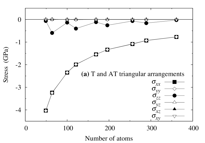
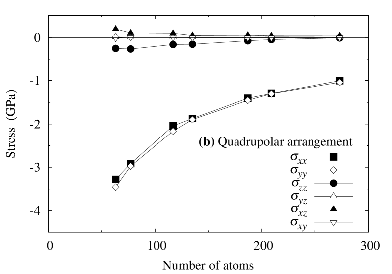
Figure 2: Homogeneous stress observed in ab initio calculations for the three periodic dislocation arrangements in the easy core configuration: (a) T and AT triangular; (b) quadrupolar dislocation arrangements.

A homogeneous stress is observed in the ab initio calculations, when the periodicity vectors are kept fixed, and when only the atomic positions are relaxed. The six components of the corresponding stress tensor are shown in Fig. 2 for the three periodic dislocation arrangements, in the easy core configuration. The stress components are expressed in the axes $\mathbf{e}_{x}=\left[\bar{1}\bar{1}{2}\right]$, $\mathbf{e}_{y}=\left[1\bar{1}0\right]$ and $\mathbf{e}_{z}=\left[111\right]$. The main components of the stress tensor are $\sigma_{xx}$ and $\sigma_{yy}$, and the other components can be neglected. The stress components $\sigma_{xx}$ and $\sigma_{yy}$ vary roughly linearly with the inverse of the number of atoms, and so with the inverse of the surface $S$ of the simulation box. For the two variants of the triangular arrangement, T and AT, the stress components $\sigma_{xx}$ and $\sigma_{yy}$ are exactly equal [Fig. 2(a)]. Indeed, the threefold symmetry along the $[111]$ direction obeyed by this dislocation arrangement is also imposed to the homogeneous stress. On the other hand, the quadrupolar arrangement breaks this symmetry. As a consequence, $\sigma_{xx}$ and $\sigma_{yy}$ slightly differ from each other in this case [Fig. 2(b)].

The two core fields of the dislocations composing the dipole are responsible for this homogeneous stress, as shown in Ref. Clouet et al., 2009. If $M_{ij}$ is the first moment tensor of the line force distribution representative of the core field, the homogeneous stress in the simulation box is given by Clouet et al. (2009)

$$\sigma_{ij}=-2\frac{M_{ij}}{S}.$$ (1)

The factor of 2 in this equation arises from the fact that two dislocations constituting the dipole are introduced within the simulation box.

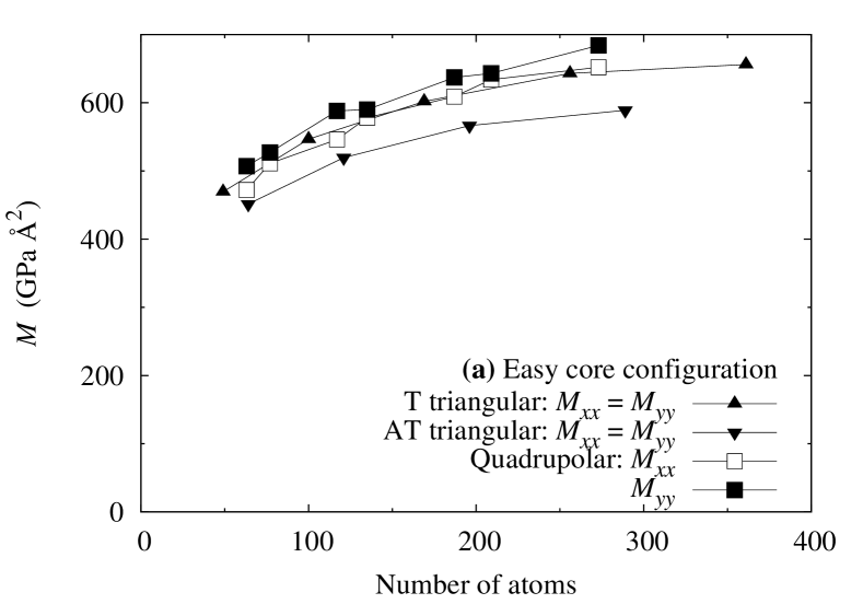
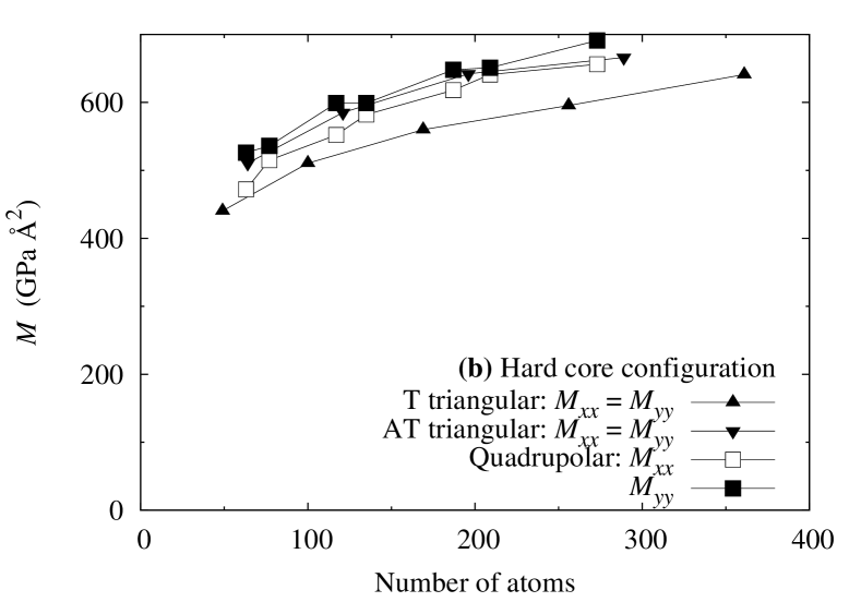
Figure 3: Moments $M_{xx}$ and $M_{yy}$ of the line force dipoles for the three periodic dislocation arrangements in the (a) easy and (b) hard core configuration.

As the stress components other than $\sigma_{xx}$ and $\sigma_{yy}$ can be neglected, the force moment tensor $M$ will have only two non-zero components, $M_{xx}$ and $M_{yy}$, as shown in Eq. (1). These two components deduced from the stress computed from DFT calculations are represented in Fig. 3(a) for the easy core configuration, and in Fig. 3(b) for the hard core configuration. Within the two triangular arrangements, the core field is a pure biaxial dilatation ($M_{xx}=M_{yy}$), whereas the core field has a small distortion component ($M_{xx}-M_{yy}\neq 0$) within the quadrupolar arrangement. This distortion is associated with the broken threefold symmetry within the quadrupolar periodic arrangement. It may arise from a polarizability Dederichs et al. (1978); Schober (1984); Puls and Woo (1986) of the core field: the moments $M$ characterizing the core field may depend on the stress applied to the dislocation core. Such a polarizability may also be the reason why the moments obtained within the T variant of the triangular arrangement slightly differ from the moments obtained within the AT variant (Fig. 3).

One can also observe a dependence of the moments with the size of the simulation box. The cell size that can be reached in DFT does not allow us to obtain well-converged values for the moments. Nevertheless, the core field of the screw dislocation in iron can be considered as a pure biaxial dilatation of amplitude $M_{xx}=M_{yy}=650\pm 50$ GPa Ų. Interestingly, the easy and the hard core configurations are characterized by the same moments [Figs. 3(a) and 3(b)], although the atomic structures of the dislocation cores are completely different between these two configurations. This probably indicates that the dislocation core field does not arise from perturbations due to the atomic nature of the core, but rather from the anharmonicity of the elastic behavior.

III.2 Simulations with relaxed periodicity vectors

Ab initio simulations, in which the periodicity vectors are allowed to relax so as to minimize the energy, have also been performed. In this case, a homogeneous strain, $\varepsilon^{0}_{ij}$, can be computed. This strain is related to the core field of the two dislocations within the simulation box, through the relation Clouet et al. (2009)

$$\varepsilon^{0}_{ij}=2S_{ijkl}\frac{M_{kl}}{S},$$

where the elastic compliances $S_{ijkl}$ are the inverse of the elastic constants. If the dislocation core field is assumed to be an elliptical line source of expansion characterized by the two non-zero moments $M_{xx}$ and $M_{yy}$, the six components of the homogeneous strain are given by

$$\begin{split}\varepsilon_{xx}^{0}&=\frac{C^{{}^{\prime}}_{33}}{C^{{}^{\prime}}_{33}(C^{{}^{\prime}}_{11}+C^{{}^{\prime}}_{12})-2{C^{{}^{\prime}}_{13}}^{2}}\frac{M_{xx}+M_{yy}}{S}\\ &+\frac{C^{{}^{\prime}}_{44}}{C^{{}^{\prime}}_{44}(C^{{}^{\prime}}_{11}-C^{{}^{\prime}}_{12})-2{C^{{}^{\prime}}_{15}}^{2}}\frac{M_{xx}-M_{yy}}{S},\\ \varepsilon_{yy}^{0}&=\frac{C^{{}^{\prime}}_{33}}{C^{{}^{\prime}}_{33}(C^{{}^{\prime}}_{11}+C^{{}^{\prime}}_{12})-2{C^{{}^{\prime}}_{13}}^{2}}\frac{M_{xx}+M_{yy}}{S}\\ &-\frac{C^{{}^{\prime}}_{44}}{C^{{}^{\prime}}_{44}(C^{{}^{\prime}}_{11}-C^{{}^{\prime}}_{12})-2{C^{{}^{\prime}}_{15}}^{2}}\frac{M_{xx}-M_{yy}}{S},\\ \varepsilon_{zz}^{0}&=-\frac{2C^{{}^{\prime}}_{13}}{C^{{}^{\prime}}_{33}(C^{{}^{\prime}}_{11}+C^{{}^{\prime}}_{12})-2{C^{{}^{\prime}}_{13}}^{2}}\frac{M_{xx}+M_{yy}}{S},\\ \varepsilon_{yz}^{0}&=0,\\ \varepsilon_{xz}^{0}&=-\frac{C^{{}^{\prime}}_{15}}{C^{{}^{\prime}}_{44}(C^{{}^{\prime}}_{11}-C^{{}^{\prime}}_{12})-2{C^{{}^{\prime}}_{15}}^{2}}\frac{M_{xx}-M_{yy}}{S},\\ \varepsilon_{xy}^{0}&=0,\end{split}$$ (2)

where the elastic constants $C^{{}^{\prime}}_{nm}$ are expressed in Voigt notation, in the axes $\mathbf{e}_{x}=\left[\bar{1}\bar{1}{2}\right]$, $\mathbf{e}_{y}=\left[1\bar{1}0\right]$, and $\mathbf{e}_{z}=\left[111\right]$. This shows that, for positive moments $M_{xx}$ and $M_{yy}$, a dilatation perpendicular to the dislocation and a contraction parallel to the dislocation line are produced. This exactly corresponds to what we observe in the ab initio calculations. Thus one can define a dislocation formation volume perpendicular to the dislocation line, $\delta V_{\bot}=(\varepsilon_{xx}^{0}+\varepsilon_{yy}^{0})S/2$ and a formation volume parallel to the dislocation line, $\delta V_{\parallel}=\varepsilon_{zz}^{0}S/2$, where the values of the formation volume are defined per unit of dislocation line. The DFT results are given in Table 1. The expressions of the homogeneous strain [Eq. (2)] also lead to a ratio between the two dislocation formation volumes depending only on the elastic constants as

$$\frac{\delta V_{\bot}}{\delta V_{\parallel}}=-\frac{C^{{}^{\prime}}_{33}}{C^{{}^{\prime}}_{13}}.$$

Using the values of the elastic constants calculated in DFT, we predict $\delta V_{\bot}/\delta V_{\parallel}=-2.0$. This is in reasonably good agreement with the values obtained from the homogeneous strain computed in ab initio calculations (Table 1).

Table 1: Formation volumes $\delta V_{\bot}$ perpendicular and $\delta V_{\parallel}$ parallel to the dislocation line per unit of dislocation line computed in DFT for the three dislocation arrangements. $N$ is the number of atoms contained within the simulation box. $M_{xx}$ and $M_{yy}$ are the moments of the dislocation core field deduced from the components $\varepsilon^{0}_{xx}$ and $\varepsilon^{0}_{yy}$ of the homogeneous strain.

	$N$	$\delta V_{\bot}$	$\delta V_{\parallel}$	$\delta V_{\bot}/\delta V_{\parallel}$	$M_{xx}$	$M_{yy}$
		(Å2)	(Å2)		(GPa Å2)	(GPa Å2)
T tri.	169	4.0	–1.5	–2.7	551	545
AT tri.	121	3.4	–1.2	–2.8	463	463
AT tri.	196	3.9	–1.2	–3.1	530	545
quadru.	135	3.9	–1.4	–2.8	527	541

(a) Easy core configuration

	$N$	$\delta V_{\bot}$	$\delta V_{\parallel}$	$\delta V_{\bot}/\delta V_{\parallel}$	$M_{xx}$	$M_{yy}$
		(Å2)	(Å2)		(GPa Å2)	(GPa Å2)
T tri.	169	3.5	–1.3	–2.6	488	465
AT tri.	121	3.9	–1.3	–3.0	531	531
AT tri.	196	4.6	–1.6	–2.9	646	619
quadru.	135	3.7	–1.3	–2.7	518	493

(b) Hard core configuration

The moments $M_{xx}$ and $M_{yy}$ characterizing the dislocation core field can be deduced from the homogeneous strain computed in DFT, using the system of equations (2). We choose to derive $M_{xx}$ and $M_{yy}$ from the components $\varepsilon_{xx}$ and $\varepsilon_{yy}$ of the strain, and the resulting values are given in Table 1 for the three arrangements. These values are in good agreement with those derived from atomistic simulations with fixed periodicity vectors (Sec. III.1). For all periodic arrangements of dislocations, the dislocation core field can be considered as a pure biaxial dilatation, and we neglect the difference between $M_{xx}$ and $M_{yy}$.

IV Core field in atomistic simulations

Now that the dislocation core field has been characterized, we examine its influence on atomistic simulations. First we look at the atomic displacements observed in ab initio calculations: part of this displacement arises from the core field. Then we show that the dislocation core energies can be extracted from these calculations when the core field contribution is considered in the elastic energy.

IV.1 Atomic displacement

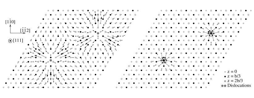
(c) T triangular periodic arrangement (361 atoms).

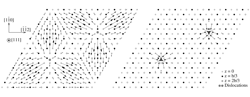
(d) AT triangular periodic arrangement (289 atoms).

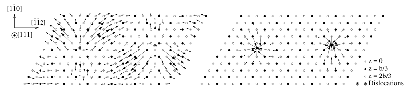
(e) Quadrupolar periodic arrangement (209 atoms).

Figure 4: Planar displacement map of a periodic unit cell containing a screw dislocation dipole in the easy core configuration, as obtained from ab initio calculations (left), and after subtraction of the Volterra and the core elastic fields (right). Vectors correspond to the $(111)$ in-plane displacement and have been magnified by a factor of 50. Displacements smaller than 0.01 Å are omitted. For clarity, displacements of the six atoms belonging to the dislocation cores are not shown on right panel.

Relaxation of atomic positions in ab initio calculations leads to the definition of atomic displacements induced by the periodic array of dislocation dipole. The displacement along the $[111]$ direction, i.e. along the dislocation line, also called the screw component, is very close to the anisotropic elastic solution corresponding to the Volterra field. There is no substantial contribution of the core field on this displacement component.

A displacement perpendicular to the dislocation line can also be evidenced in atomistic simulations, i.e. an edge component (Fig. 4). Part of this displacement component corresponds to the dislocation Volterra field and arises from elastic anisotropy. The dislocation core field also contributes to the edge component. The Volterra contribution is more long-ranged than the core field contribution, as the former varies with the logarithm of the distance to the dislocation, whereas the latter varies with the inverse of this distance. Nevertheless, both contributions evidence a similar amplitude in the simulations, because of the reduced cell size used in DFT calculations.

We can subtract from the atomic displacement given by ab initio calculations, the displacement corresponding to the superposition of the Volterra and the dislocation core fields, as predicted by the anisotropic linear elasticity taking full account of the periodic boundary conditions Cai et al. (2003). The resulting map, represented in Fig. 4, shows that the elastic modeling manages to reproduce the ab initio displacements for all periodic arrangements even close to the dislocation core. The anisotropic linear elasticity fails to reproduce the ab initio atomic displacement only on the atoms within the core: displacements in the core are too large for applying a small perturbation theory such as elasticity.

IV.2 Dislocation core energy

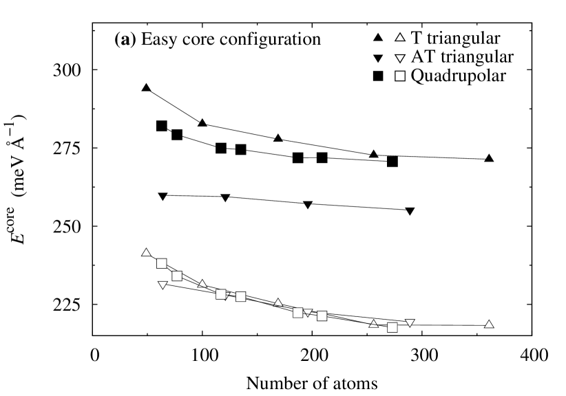
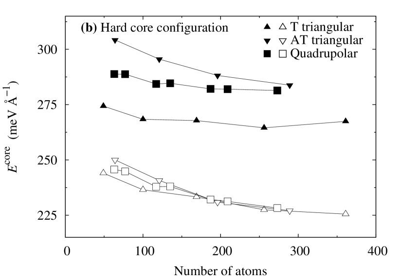
Figure 5: Core energy of the screw dislocation in the (a) easy and the (b) hard core configuration. Solid symbols correspond to the core energies obtained when only the Volterra field is considered, and open symbols, to the core energies when both the Volterra and the core fields are taken into account ($r_{\rm c}=3$ Å).

The screw dislocation core energy is deduced from DFT simulations by subtracting the elastic energy to the excess energy of the unit cell computed by ab initio techniques. The elastic energy is calculated by taking into account the elastic anisotropy and the periodic boundary conditions Cai et al. (2003).

If only the Volterra contribution is considered in the elastic energy, the resulting core energies strongly depend on the periodic arrangement (Fig. 5). As shown in Ref. Clouet et al., 2009, one can not conclude on the relative stability of the two different core configurations of the screw dislocation. The AT triangular geometry and the quadrupolar geometry predict that the easy core is the most stable configuration, whereas the T triangular arrangement leads to the opposite conclusion. Then if both the Volterra and the core fields are considered in the elastic energy, the core energies do not depend anymore on the periodic arrangement. A cell size dependence has been evidenced (Fig. 5), and in all geometries the easy core is more stable than the hard core configuration. The convergence is reached for a reasonable number of atoms: $E^{\rm core}=219\pm 1$ meV Å^-1 for the easy core configuration, and $227\pm 1$ meV Å^-1 for the hard core configuration. These core energies are given for a core radius $r_{\rm c}=3$ Å, as this value of $r_{\rm c}$ has been found to lead to a reasonable convergence of the core energy with respect to the cell size (cf. Appendix A).

To better understand how the core energy converges, one can decompose the elastic energy into the different contributions, and look how these contributions vary with the length scale. If one neglects the dislocation core field, the elastic energy of the simulation box containing a dislocation dipole is given by

$$E^{\rm elas}_{\rm V}=2E^{\rm elas}_{\rm c}+b_{i}K^{0}_{ij}b_{j}\ln{\left(A/r_{\rm c}\right)}+E^{\rm inter}_{\rm V-V},$$ (3)

where $K^{0}$ is a second rank tensor, which depends only on the elastic constants, and $r_{\rm c}$ is the dislocation core cutoff. The two first terms on the right hand side define the elastic energy of the dipole contained in the simulation box: $E^{\rm elas}_{\rm c}$ is the core traction contribution Clouet (2009), and the second term corresponds to the cut contribution. $E^{\rm inter}_{\rm V-V}$ corresponds to the interaction of the dislocation dipole with its periodic images Cai et al. (2003). If the core field is taken into account Clouet (2011), the elastic energy becomes

$$E^{\rm elas}=E^{\rm elas}_{\rm V}+M_{ij}K^{2}_{ijkl}M_{kl}\frac{1}{{r_{\rm c}}^{2}}+2E^{\rm inter}_{\rm V-c}+E^{\rm inter}_{\rm c-c},$$ (4)

where the fourth rank tensor $K^{2}$, which only depends on the elastic constants, enables one to calculate the core field contribution to the dislocation self energy. $E^{\rm inter}_{\rm V-c}$ and $E^{\rm inter}_{\rm c-c}$ correspond to the interaction of the dislocation core field with respectively the Volterra field, and the core field of the other dislocations, i.e. the second dislocation composing the dipole, as well as the image dislocations due to the periodic boundary conditions. When the periodicity vectors, $\mathbf{u}$ and $\mathbf{v}$, and the dipole cut, $\mathbf{A}$, are scaled by the same factor $\lambda$, $E^{\rm inter}_{\rm V-c}$ varies as $1/\lambda$, and $E^{\rm inter}_{\rm c-c}$, as $1/\lambda^{2}$. The number $N$ of atoms in the simulation box is proportional to $\lambda^{2}$. The comparison of equations (3) and (4) shows then that the neglect of the core field leads to a core energy that converges as $N^{-1/2}$. In the case of dislocation periodic arrangements, which are centrosymmetric like the quadrupolar arrangement of Fig. 1(c), $E^{\rm inter}_{\rm V-c}$ vanishes in Eq. (4). The core energy converges thus as $N^{-1}$ when the core field is neglected. In all cases, this convergence is too slow to extract a meaningful core energy from ab initio calculations. Moreover, the obtained value does not really correspond to the core energy $E^{\rm core}$: it results from the summation of $E^{\rm core}$ and the core field self elastic energy, $M_{ij}K^{2}_{ijkl}M_{kl}1/{r_{\rm c}}^{2}$.

Another interesting feature comes from the linear dependency of $E^{\rm inter}_{\rm V-c}$ with the Burgers vector. Going from the easy to the hard core configuration of the dislocation dipole, i.e. inverting the sign of the Burgers vector, one only changes the sign of $E^{\rm inter}_{\rm V-c}$, whereas all other contributions to the elastic energy remain constant. The easy and the hard core configurations have indeed a core field with the same amplitude (Fig. 3). The contribution $E^{\rm inter}_{\rm V-c}$ is positive for a dislocation dipole in its easy core configuration within the T triangular arrangement [Fig. 1(a)]. Therefore, when the core field contribution is not included into the elastic energy, one underestimates the stability of the easy core configuration with respect to the hard core configuration within this geometry. The AT triangular arrangement leads to the opposite conclusion [Fig. 1(b)], since $E^{\rm inter}_{\rm V-c}$ becomes negative for the easy core configuration.

The underestimation or overestimation of the stability of the easy core illustrates the importance of considering the dislocation core field in the elastic energy, when extracting quantitative properties from atomistic simulations. This is especially true for ab initio calculations, in which the small cell size makes it difficult to obtain converged values. Such a conclusion is not restricted to the calculation of dislocation core energies. For instance, extraction from atomistic simulations of the Peierls energy barriers, and of the associated Peierls stresses, will also require the complete modeling of the dislocation core field.

IV.3 Dislocation line energy and line tension

It is interesting to evaluate the different contributions to the dislocation line energy. Using the developed elastic model, the energy of a straight screw dislocation contained in a cylinder of radius $R_{\infty}$ is

$$E=E^{\rm core}+E_{\rm c}^{\rm elas}+\frac{1}{2}b_{i}K^{0}_{ij}b_{j}\ln{\left(\frac{R_{\infty}}{r_{\rm c}}\right)}\\ +\frac{1}{2}M_{ij}K^{2}_{ijkl}M_{kl}\frac{1}{{r_{\rm c}}^{2}}.$$ (5)

The core energy has been found to be $E^{\rm core}=219\pm 1$ meV Å^-1 for the easy core configuration, and $227\pm 1$ meV Å^-1 for the hard core configuration, with $r_{\rm c}=3$ Å. The Volterra elastic field leads to two energy contributions: the contribution of the core traction Clouet (2009) is $E_{\rm c}^{\rm elas}=1$ meV Å^-1, for a dislocation cut corresponding to a $\{110\}$ glide plane, and the cut contribution, which corresponds to the third term in Eq. (5), is equal to 1.60 eV Å^-1, where we have assumed the ratio $R_{\infty}/r_{\rm c}=10^{4}$, which corresponds to a characteristic dislocation density of $10^{11}$ m^-2. Finally, the core field contribution to the elastic energy, which corresponds to the last term in Eq. (5), is equal to 42 meV Å^-1. It is clear that most of the dislocation energy arises from the Volterra elastic field, and is associated with the cut contribution. Other contributions, which are all associated with the dislocation core, account for about 14 % of the dislocation energy. In particular, the contribution of the core field is less than 3 %.

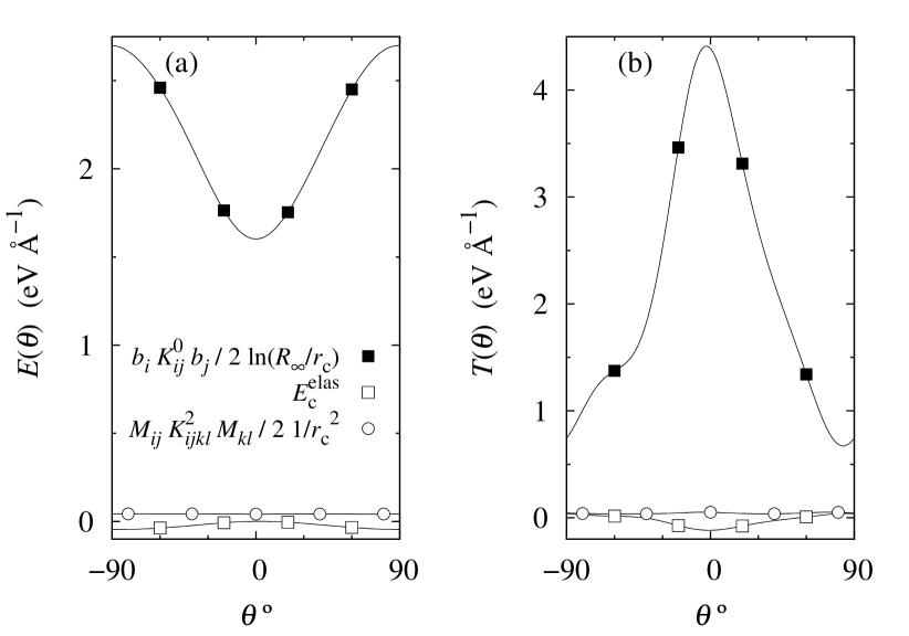
Figure 6: Elastic contributions [Eq. (5)] to the dislocation (a) line energy $E(\theta)$ and (b) line tension $T(\theta)=E(\theta)+{\mathrm{d}^{2}E(\theta)}/{\mathrm{d}\theta^{2}}$ as a function of the dislocation character $\theta$ in the $\left\{110\right\}$ glide plane. $\theta=0$ for the screw orientation.

The dislocation line tension is actually more important than the line energy as it controls the shape of dislocation loops and curved dislocationsde Wit and Koehler (1959). It is defined as

$$T(\theta)=E(\theta)+\frac{\mathrm{d}^{2}E(\theta)}{\mathrm{d}\theta^{2}},$$

if $E(\theta)$ is the dislocation line energy [Eq. (5)] written as a function of the dislocation character $\theta$, i.e. the dislocation orientation. We can evaluate this line tension by considering all elastic contributions entering in the dislocation line energy and neglecting the dependence of the dislocation core energy with $\theta$ which we do not know. For the dislocation core field, we assume that the dipole tensor $M_{ij}$ does not depend on the dislocation orientation as we do not have any information on such a variation: the variation with the dislocation orientation of the associated line energy only arises from elastic anisotropy. The different elastic contributions to the dislocation line energy $E(\theta)$ and the associated line tension $T(\theta)$ are shown in Fig. 6 for a dislocation character going from an edge orientation ($\theta=\pm 90^{\circ}$) to a screw orientation ($\theta=0$). The most important contribution to the line tension arises, once again, from the cut contribution of the Volterra elastic field. In view of the values obtained, it looks reasonable to neglect other elastic contributions, as usually done in line tension modelsde Wit and Koehler (1959). Nevertheless, some other studies have obtained higher relative contributions of the core field Gehlen et al. (1972); Hoagland et al. (1976), which may therefore have a more important effect on the line tension.

V Dislocation interaction with a carbon atom

We examine in this part how the dislocation core field influences the dislocation properties by modifying the way a dislocation can interact with its environment. First, we study the interaction between a $\langle 111\rangle$ screw dislocation and a carbon atom in $\alpha$-iron.

In Ref. Clouet et al., 2008, the binding energy between a carbon atom and a screw dislocation in iron as predicted by the linear anisotropic elasticity has been compared to the one calculated by atomistic simulations based on an empirical potential approach Becquart et al. (2007). A quantitative agreement between both modeling techniques was obtained as long as the C atom was located at a distance greater than 2 Å from the dislocation core. This result evidences the ability of linear elasticity to predict this interaction. The empirical potential for iron Mendelev et al. (2003); Ackland et al. (2004) used in Ref. Clouet et al., 2008 does not lead to any core field for the screw dislocation, at variance with the present ab initio results. It is interesting to include now the core field contribution into the elastic field of the screw dislocation, to investigate its influence on the interaction between a carbon atom and a screw dislocation. Such a contribution to the interaction energy between a solute atom and a dislocation has already been considered in the case of a substitutional impurity by FleischerFleischer (1963) who showed that it partly contributes to the solid solution hardening.

V.1 Carbon atom description

First we need to deduce from ab initio calculations a quantitative representation of a carbon atom embedded in an iron matrix. A solute atom is modeled in elasticity theory by its dipolar tensor, $P_{ij}$, which corresponds to the first moments of the equilibrated point force distribution equivalent to the impurity. This tensor is deduced from atomistic simulations of one solute atom embedded in the solvent (cf. Appendix B).

Carbon atoms are found in the octahedral interstitial sites of the bcc lattice. The dipolar tensor, $P_{ij}$, expressed in the cubic axes, is diagonal with only two independent components, because of the tetragonal symmetry of the octahedral site. Three variants can be obtained, depending on the orientation of the tetragonal symmetry axis. For the $\left[001\right]$ variant of the C atom, ab initio calculations lead to $P_{xx}=P_{yy}=8.9$ and $P_{zz}=17.5$ eV (cf. Appendix B).

V.2 Binding energy

Figure 7: Binding energy between a $1/2[111](1\bar{1}0)$ screw dislocation and a carbon atom for different positions $x$ of the dislocation in its $(1\bar{1}0)$ glide plane. The C atom lies in a [100] octahedral site in the plane $h=d_{110}\approx 2.04$ Å above the glide plane. The binding energy is calculated using the anisotropic elasticity theory considering only the Volterra field, or both the Volterra and the core fields of the dislocation.

Linear elasticity theory predicts that the binding energy between the carbon atom characterized by its dipolar tensor, $P_{ij}$, and the screw dislocation is given by

$$E^{\rm bind}=P_{ij}\varepsilon_{ij}^{\rm d},$$ (6)

where $\varepsilon_{ij}^{\rm d}$ is the elastic strain created by the dislocation. We use the linear anisotropic elasticity to calculate $\varepsilon_{ij}^{\rm d}$ by taking into account only the Volterra field, or both the Volterra and the core fields created by the dislocation. We consider that the core field is created by the line force moments $M_{xx}=M_{yy}=650$ GPa Ų previously deduced. In Fig. 7, we represent the variation of the binding energy when the dislocation glides in a $\left\{110\right\}$ plane, while the carbon atom remains at a fixed distance $h$ from the glide plane. The first derivative of the plotted function gives the force exerted by the C atom on the gliding dislocation. When the C atom is close enough to the dislocation, the core field modifies the binding energy. In particular, the binding of the C atom is stronger in the attractive region when the dislocation core field is considered. Thus the pinning of the screw dislocation by the C atom is enhanced by its core field. Conversely, the dislocation core field leads to a stronger repulsion in the repulsive region.

When the separation distance between the C atom and the screw dislocation is high enough ($\gtrsim 20$ Å), the dislocation core field does not affect anymore the binding energy. One can consider that the C atom interacts only with the dislocation Volterra field.

VI Passing properties of a screw dislocation dipole

We look in this part at how the dislocation core field modifies the equilibrium properties of a screw dislocation dipole. Dislocation dipoles play a significant role in single slip straining, where they can control the material flow stress. Such a situation arises for instance in fatigued metals, where dislocations are constrained to glide in the channels between dislocation walls Mughrabi and Pschenitzka (2005); Brown (2006). The saturation stress of the persistent slip bands is then partly controlled by the critical stress needed to destroy the dislocation dipoles.

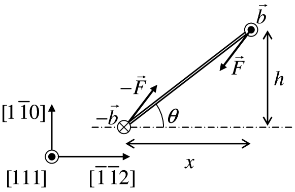
Figure 8: Screw dislocation dipole. $\mathbf{F}$ is the force exerted by one dislocation on the other.

Figure 9: Variation of the elastic energy, $\Delta E$, and of the $x$ component of the force $\mathbf{F}$ acting on the dislocations, $F_{x}$, with the distance between both dislocations, $x$, for a screw dipole of height $h=10$ Å.

We consider a screw dislocation dipole in bcc iron. The dipole is characterized by the height between each dislocation glide plane, $h$, and by the projection of the dipole vector on the glide plane, $x$, as sketched in Fig. 8. Then we calculate the variation of the interaction energy between the two dislocations composing the dipole, $\Delta E$, when dislocations glide, i.e. $h$ is kept fixed while $x$ varies. This dislocation interaction energy is computed using the linear anisotropic elasticity Clouet (2011), and considering that the two dislocations composing the dipole interact only through the Volterra field, or through both the Volterra and the core fields. This variation of energy, $\Delta E$, is represented in Fig. 9 for a dipole height $h=10$ Å. The dipole equilibrium angle corresponds to the minimum of $\Delta E$, i.e. $\theta=0$. This value predicted by the anisotropic elasticity is equal to the one given by the isotropic elasticity. This contrasts with what is found in fcc metals, where the dipole equilibrium angle strongly depends on elastic anisotropy for a screw dislocation dipole Veyssière and Chiu (2007). The dislocation core field does not modify the dipole equilibrium angle (Fig. 9). Nevertheless, when both the Volterra and the core fields are included into the computation of the dipole elastic energy, the energy that defines the dipole equilibrium becomes steeper than when the dislocation core field is omitted. Thus the attraction between both dislocations is stronger when the core field is taken into account. This is obvious when looking at the glide component of the force exerted by one dislocation on the other one, $F_{x}$ (Fig. 9). This force is the first derivative of $\Delta E$ with respect to $x$. When the dislocation core field is included in the dislocation interaction, this force goes to a higher maximum value than when only the Volterra elastic field is considered. To destroy the dislocation dipole, one needs to exert on a dislocation a force that is higher than the force arising from the interaction with the other dislocation. This shows that the dislocation core field leads to a more stable dipole.

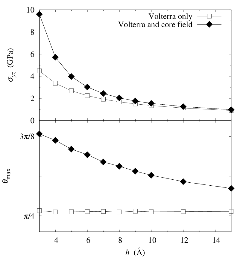
Figure 10: Variation of the passing stress, $\sigma_{yz}$, and of the passing angle, $\theta_{\rm max}$, with the dislocation dipole height, $h$.

If a homogeneous stress is applied, the gliding force on each dislocation is simply the Peach-Koehler force, $b\sigma_{yz}$. As the applied stress is homogeneous, no force originates from the dislocation core field Clouet (2011). Therefore the dipole passing stress, i.e. the applied stress needed to destroy the dislocation dipole, is given by the maximum of the glide component $F_{x}$ of the Peach-Koehler force divided by the norm of the Burgers vector. This passing stress depends on the dipole height, $h$, as shown in Fig. 10. The inclusion of the core field into the dislocation interaction leads to a higher passing stress, especially for small dipole heights. But the effect is relevant at a spacing where the dipole would certainly have cross-slipped to annihilation. For large dipole heights ($h\geq 20$ Å), the dislocation core field does not influence too much the passing stress, and one can consider that dislocations interact only through the Volterra elastic field to calculate the passing stress.

Without the dislocation core field, the dipole passing angle, $\theta_{\rm max}$, does not depend on the dipole height (Fig. 10). The value given by the anisotropic elasticity is close to the $\pi/4$ value predicted by the isotropic elasticity. The core field leads to a passing angle, which depends on the dipole height, and which strongly deviates from $\pi/4$ for small dipole heights. Such a dependence of the passing angle with the dipole height has also been obtained by Henager and Hoagland for edge dislocation dipoles in fcc metals Henager and Hoagland (2004, 2005). They obtained a stronger influence of the core field on the dislocation interaction than in the present study. In their case, the core field contribution can be neglected only when the two dislocations are separated by more than $50b$, i.e. more than 10 nm.

VII Conclusions

The approach developed in the preceding paper to model dislocation core field Clouet (2011), has been applied here to the $\langle 111\rangle$ screw dislocation in $\alpha$-iron. Using ab initio calculations, we have shown that a screw dislocation creates a core field corresponding to a dilatation perpendicular to the dislocation line. The core field modeling within the anisotropic linear elasticity perfectly reproduces the atomic displacements observed in ab initio calculations. It also allows to derive from atomistic simulations converged values of the dislocation core energies. The developed approach illustrates the necessity to consider the dislocation core field when extracting quantitative information from atomistic simulations of dislocations.

Then the elastic modeling of the screw dislocation has been used to study the interaction energy between the dislocation and a carbon atom. The dislocation core field increases the binding of the C atom when both defects are close enough (less than $\sim$20 Å). At larger separation distances, the C atom interacts only with the dislocation Volterra elastic field.

Equilibrium properties of a screw dislocation dipole are also affected by the dislocation core field. This additional elastic field increases the stability of the dipole: a higher stress is needed to destroy the dipole. Nevertheless, when the two dislocations composing the dipole are sufficiently separated, one can consider that they only interact through their Volterra field.

The amplitude of the dilatation corresponding to the dislocation core field does not depend on the dislocation core configuration, i.e. either easy or hard core structure. This indicates that the core field does not arise from the atomic structure of the dislocation core, but may be induced by anharmonicity. Our work, like previous similar studies Henager and Hoagland (2004, 2005); Gehlen et al. (1972); Hirth and Lothe (1973); Hoagland et al. (1976); Sinclair et al. (1978), shows that such an anharmonic effect can be fully considered within linear elasticity theory with the help of a localized core field. One could have also used non-linear elasticity theory to incorporate anharmonic contributions, either following the approach of Seeger and Haasen Seeger and Haasen (1958) based on a Grüneisen model for an isotropic crystal, or the iterative scheme proposed by Willis Willis (1967); Teodosiu (1982) for an anisotropic crystal.

Appendix A Core energies and core radius

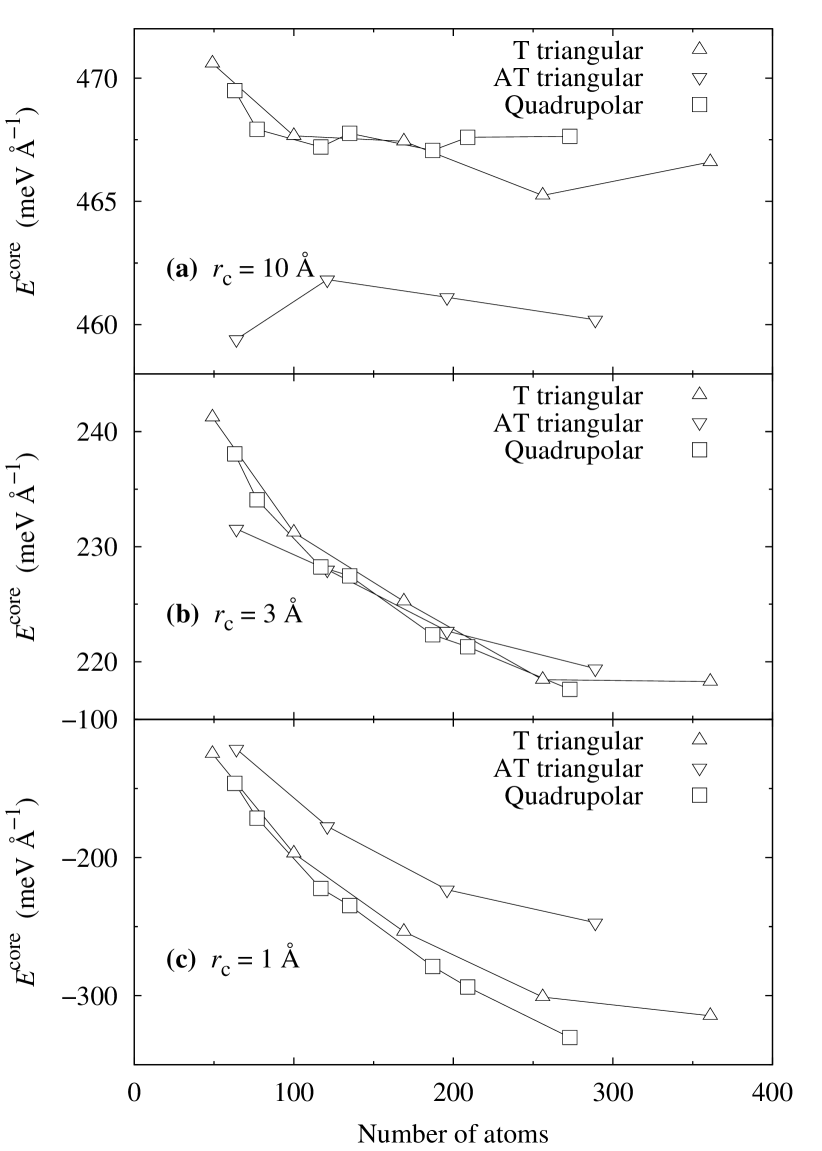
Figure 11: Core energy of the screw dislocation in the easy core configuration for different core radii: (a) $r_{\rm c}=10$ Å, (b) $r_{\rm c}=3$ Å, and (c) $r_{\rm c}=1$ Å. Both the Volterra and the core fields have been considered in the elastic energy.

The core energy depends on the choice of the core radius $r_{\rm c}$. This core radius defines the cylindrical region around the dislocation line, where the strain is so high that elasticity theory does not apply. It therefore partitions the dislocation excess energy into two contributions, the core energy corresponding to the energy stored in this core cylinder and the elastic energy in the remaining space. Changing the value of $r_{\rm c}$ modifies this partition between core and elastic energy without modifying the total excess energy [Eq. (5)]. In the present work, the choice of $r_{\rm c}$ affects the convergence of the core energy with the size of the simulation box and the geometry of the dislocation periodic array. This arises from the dislocation core field. The dislocation line energy created by this core field depends on $r_{\rm c}$ through the contribution $1/2\ M_{ij}K_{ijkl}M_{kl}\ 1/{r_{\rm c}}^{2}$ [Eq. (5)]. As the dipole moments $M_{ij}$ have been found to depend on the size of the simulation cell (Fig. 3), changing the value of $r_{\rm c}$ leads to a shift of the core energy which also depends on this size. Figure 11 shows the core energies obtained for different core radii. One sees that the value $r_{\rm c}=3$ Å leads to a core energy which does not depend on the geometry of the dislocation periodic array and which converges reasonably with the size of the simulation cell. Moreover, it is close to the norm of the Burgers vector ($b=2.5$ Å) as theoretically expectedHirth and Lothe (1982).

Appendix B Carbon dipolar tensor

Figure 12: Variation of the stress $\sigma_{ij}$ and of the corresponding dipolar tensor $P_{ij}$ with the inverse of the volume $V$ of a unit cell containing one C atom in a [001] variant embedded in an Fe matrix. Symbols correspond to ab initio calculations and solid lines to Eq. (7) and (8).

A solute C atom embedded in a Fe matrix is modeled within elasticity theory by a dipolar tensorBacon et al. (1980) $P_{ij}$. As shown in Ref. Clouet et al., 2008, the value of this tensor can be simply deduced from the stress tensor measured in atomistic simulations where one solute atom is embedded in the solvent using periodic boundary conditions. One predicts that the homogeneous stress measured in these simulations varies linearly with the inverse of the volume $V$ of the unit cell,

$$\sigma_{ij}=-\frac{P_{ij}}{V}.$$

Because of the small size of the unit cell used in ab initio calculations, one has to take into account the polarizabilityDederichs et al. (1978); Schober (1984); Puls and Woo (1986) of the C atom, i.e. the fact that the tensor $P_{ij}$ depends of the strain $\varepsilon_{kl}^{\rm C}$ locally applied on the C atom. One can write to first order

$$P_{ij}\left(\varepsilon_{kl}^{\rm C}\right)=P^{0}_{ij}+P^{1}_{ijkl}\varepsilon_{kl}^{\rm C},$$

where $P^{0}_{ij}$ is the C dipolar tensor in an unstrained crystal and $P^{1}_{ijkl}$ its first derivative with respect to the applied strain. In our atomistic simulations, this applied strain $\varepsilon_{kl}^{\rm C}$ arises from the periodic images of the C atom. The strain created by a point defect varies linearly with the inverse of the cube of the separation distance and we use for our atomistic simulations homothetic unit cells with the same cubic shape. The dipolar tensor $P_{ij}$ should therefore vary linearly with the inverse of the volume of the unit cell,

$$P_{ij}=P^{0}_{ij}+\frac{\delta P_{ij}}{V},$$ (7)

where $\delta P_{ij}$ is a constant depending only on the shape of the unit cell and not on its volume. As a consequence, the stress measured in the atomistic simulations should vary like

$$\sigma_{ij}=-\frac{P^{0}_{ij}}{V}-\frac{\delta P_{ij}}{V^{2}}.$$ (8)

We performed ab initio calculations to obtain the values of the dipolar tensor, characterizing one carbon atom in the iron matrix. We chose a cubic unit cell which contains one C atom in an octahedral interstitial site. The simulation boxes contain 128, 250, or 432 Fe atoms. The Siesta calculation details are the same as for dislocation calculations, and 13 numerical pseudoatomic orbitals per carbon atom are used to represent the valence electrons as described in Ref. Fu et al., 2008. The k-point grids used for the calculations are $4\times 4\times 4$ for the 128 and 250 atom cells and $3\times 3\times 3$ for the 432 atom cells.

Because of the tetragonal symmetry of the octahedral interstitial site, the dipolar tensor characterizing the C atom is diagonal with only two independent components. This agrees with the symmetry of the stress tensor given by ab initio calculations. The variations of this stress tensor with the volume of the unit cell are in perfect agreement with Eq. (8) (Fig. 12). This allows us to deduce the elastic dipole $P_{ij}$ which is characterized by the values $P_{xx}=P_{yy}=8.9$ and $P_{zz}=17.5$ eV for the [100] variant of the C atom in the dilute limit [$V\rightarrow\infty$ in Eq. (7)].

Previous ab initio calculations performed in smaller simulation cells have led to the C atom dipolar tensor deduced from Kanzaki forces Domain et al. (2004). These values are consistent with the ones we have deduced from the homogeneous stress.

Table 2: Variations of the iron lattice parameter with carbon atomic fraction, $\delta_{x}$ and $\delta_{z}$, and formation volume of carbon, $\delta\Omega$.

	$\delta_{x}$	$\delta_{z}$	$\delta\Omega$ (Å3)
Ab initio	–0.086	1.04	10.4
Empirical potential Becquart et al. (2007)	–0.088	0.56	4.47
Exp. Cochardt et al. (1955)	–0.052	0.76	7.63
Exp. Bacon (1969)	–0.0977	0.862	7.76
Exp. Cheng et al. (1990)	–0.09	0.85	7.80

The elastic dipole, $P_{ij}$, can be simply related to the parameters $\delta_{x}$ and $\delta_{z}$ of the Vegard law Clouet et al. (2008), which assumes a linear relation between the variations of the lattice parameter, $a$ and $c$, and the atomic fraction of carbon atoms, $x_{\rm C}$. If all carbon atoms are located on the $\left[001\right]$ variant of the octahedral site,

$$\begin{split}a(x_{\rm C})&=a_{0}\left(1+\delta_{x}x_{\rm C}\right)\textrm{, along the $\left[100\right]$ or $\left[010\right]$ axis,}\\ c(x_{\rm C})&=a_{0}\left(1+\delta_{z}x_{\rm C}\right)\textrm{, along the $\left[001\right]$ axis,}\end{split}$$

where $a_{0}$ is the pure Fe lattice parameter. The parameters $\delta_{x}$ and $\delta_{z}$ deduced from our DFT calculations are compared to experimental data Cochardt et al. (1955); Bacon (1969); Cheng et al. (1990) in Table 2. The ab initio calculations lead to a formation volume of carbon larger than the experimental value, and to a larger tetragonal distortion expressed as $(\delta_{z}-\delta_{x})$.

One can also deduce from the elastic dipole the variation of the solution enthalpy of C in bcc Fe with a volume expansion,

$$V_{0}\left.\frac{\partial H^{\rm exc}}{\partial V}\right|_{V=V_{0}}=-\frac{1}{3}P_{ii},$$

where $H^{\rm exc}$ is the excess enthalpy of a Fe crystal of equilibrium volume $V_{0}$ containing one C atom. The value corresponding to the elastic dipoles calculated above, $-11.8$ eV, is in good agreement with the value obtained by Hristova et al. Hristova et al. (2011), $-12.3$ eV, using an ab initio approach based on GGA-DFT with a plane waves basis set and the Blöchl projector-augmented wave method (PAW) as implemented in the Vienna Ab Initio Simulation Package (VASP). This validates our Siesta approach for characterizing C atom embedded in an iron bcc matrix.

References

- Clouet et al. (2009) E. Clouet, L. Ventelon, and F. Willaime, Phys. Rev. Lett., 102, 055502 (2009).
- Ismail-Beigi and Arias (2000) S. Ismail-Beigi and T. A. Arias, Phys. Rev. Lett., 84, 1499 (2000).
- Frederiksen and Jacobsen (2003) S. L. Frederiksen and K. W. Jacobsen, Philos. Mag., 83, 365 (2003).
- Gehlen et al. (1972) P. C. Gehlen, J. P. Hirth, R. G. Hoagland, and M. F. Kanninen, J. Appl. Phys., 43, 3921 (1972).
- Hoagland et al. (1976) R. G. Hoagland, J. P. Hirth, and P. C. Gehlen, Philos. Mag., 34, 413 (1976).
- Woo and Puls (1977) C. H. Woo and M. P. Puls, Philos. Mag., 35, 727 (1977).
- Henager and Hoagland (2004) C. H. Henager and R. G. Hoagland, Scripta Mater., 50, 1091 (2004).
- Henager and Hoagland (2005) C. H. Henager and R. G. Hoagland, Philos. Mag., 85, 4477 (2005).
- Hirth and Lothe (1973) J. P. Hirth and J. Lothe, J. Appl. Phys., 44, 1029 (1973).
- Clouet (2011) E. Clouet, Phys. Rev. B, 84, 224111 (2011).
- Ventelon and Willaime (2007) L. Ventelon and F. Willaime, J. Computer-Aided Mater. Des., 14, 85 (2007).
- Vitek (1974) V. Vitek, Crystal Latt. Def., 5, 1 (1974).
- Lehto and Öberg (1998) N. Lehto and S. Öberg, Phys. Rev. Lett., 80, 5568 (1998).
- Cai et al. (2001) W. Cai, V. V. Bulatov, J. Chang, J. Li, and S. Yip, Phys. Rev. Lett., 86, 5727 (2001).
- Cai et al. (2003) W. Cai, V. V. Bulatov, J. Chang, J. Li, and S. Yip, Philos. Mag., 83, 539 (2003).
- Li et al. (2004) J. Li, C.-Z. Wang, J.-P. Chang, W. Cai, V. V. Bulatov, K.-M. Ho, and S. Yip, Phys. Rev. B, 70, 104113 (2004).
- Soler et al. (2002) J. M. Soler, E. Artacho, J. D. Gale, A. García, J. Junquera, P. Ordejón, and D. Sánchez-Portal, J. Phys.: Condens. Matter, 14, 2745 (2002).
- Fu et al. (2004) C.-C. Fu, F. Willaime, and P. Ordejón, Phys. Rev. Lett., 92, 175503 (2004).
- Ventelon and Willaime (2010) L. Ventelon and F. Willaime, Philos. Mag., 90, 1063 (2010).
- Note (1) One can also consider a distribution of dislocation dipoles to model the core field. We found that the core field representation as a line force distribution works better for the screw dislocation in iron, and therefore we did not consider any dislocation dipole in the core field.
- Dederichs et al. (1978) P. Dederichs, C. Lehmann, H. Schober, A. Scholz, and R. Zeller, J. Nucl. Mater., 69-70, 176 (1978).
- Schober (1984) H. R. Schober, J. Nucl. Mater., 126, 220 (1984).
- Puls and Woo (1986) M. P. Puls and C. H. Woo, J. Nucl. Mater., 139, 48 (1986).
- Note (2) .
- Clouet (2009) E. Clouet, Philos. Mag., 89, 1565 (2009).
- Note (3) The different energy contributions have been calculated for a core radius \tmspace+.1667emÅ.
- de Wit and Koehler (1959) G. de Wit and J. S. Koehler, Phys. Rev., 116, 1113 (1959).
- Clouet et al. (2008) E. Clouet, S. Garruchet, H. Nguyen, M. Perez, and C. S. Becquart, Acta Mater., 56, 3450 (2008).
- Becquart et al. (2007) C. S. Becquart, J. M. Raulot, G. Bencteux, C. Domain, M. Perez, S. Garruchet, and H. Nguyen, Comp. Mater. Sci., 40, 119 (2007).
- Mendelev et al. (2003) M. I. Mendelev, S. Han, D. J. Srolovitz, G. J. Ackland, D. Y. Sun, and M. Asta, Philos. Mag., 83, 3977 (2003).
- Ackland et al. (2004) G. J. Ackland, M. I. Mendelev, D. J. Srolovitz, S. Han, and A. V. Barashev, J. Phys.: Condens. Matter, 16, S2629 (2004).
- Fleischer (1963) R. L. Fleischer, Acta Metall., 11, 203 (1963).
- Mughrabi and Pschenitzka (2005) H. Mughrabi and F. Pschenitzka, Philos. Mag., 85, 3029 (2005).
- Brown (2006) L. M. Brown, Philos. Mag., 86, 4055 (2006).
- Veyssière and Chiu (2007) P. Veyssière and Y.-L. Chiu, Philos. Mag., 87, 3351 (2007).
- Sinclair et al. (1978) J. E. Sinclair, P. C. Gehlen, R. G. Hoagland, and J. P. Hirth, J. Appl. Phys., 49, 3890 (1978).
- Seeger and Haasen (1958) A. Seeger and P. Haasen, Philos. Mag., 3, 470 (1958).
- Willis (1967) J. R. Willis, Int. J. Eng. Sci., 5, 171 (1967).
- Teodosiu (1982) C. Teodosiu, Elastic Models of Crystal Defects (Springer-Verlag, Berlin, 1982).
- Hirth and Lothe (1982) J. P. Hirth and J. Lothe, Theory of Dislocations, 2nd ed. (Wiley, New York, 1982).
- Bacon et al. (1980) D. J. Bacon, D. M. Barnett, and R. O. Scattergood, Prog. Mater. Sci., 23, 51 (1980).
- Fu et al. (2008) C. C. Fu, E. Meslin, A. Barbu, F. Willaime, and V. Oison, Solid State Phenom., 139, 157 (2008).
- Domain et al. (2004) C. Domain, C. S. Becquart, and J. Foct, Phys. Rev. B, 69, 144112 (2004).
- Cochardt et al. (1955) A. W. Cochardt, G. Schoek, and H. Wiedersich, Acta Metall., 3, 533 (1955).
- Bacon (1969) D. J. Bacon, Scripta Metall., 3, 735 (1969).
- Cheng et al. (1990) L. Cheng, A. Bottger, T. H. de Keijser, and E. J. Mittemeijer, Scripta Metall. Mater., 24, 509 (1990).
- Hristova et al. (2011) E. Hristova, R. Janisch, R. Drautz, and A. Hartmaier, Comp. Mater. Sci., 50, 1088 (2011).