Pseudospin for Raman $D$ Band in Armchair Graphene Nanoribbons

Abstract

By analytically constructing the matrix elements of an electron-phonon interaction for the $D$ band in the Raman spectra of armchair graphene nanoribbons, we show that pseudospin and momentum conservation result in (i) a $D$ band consisting of two components, (ii) a $D$ band Raman intensity that is enhanced only when the polarizations of the incident and scattered light are parallel to the armchair edge, and (iii) the $D$ band softening/hardening behavior caused by the Kohn anomaly effect is correlated with that of the $G$ band. Several experiments are mentioned that are relevant to these results. It is also suggested that pseudospin is independent of the boundary condition for the phonon mode, while momentum conservation depends on it.

I Introduction

Raman spectroscopy has been widely used for the characterization of carbon-based materials such as graphite, graphene, nanotubes, and nanoribbons. Malard et al. (2009) Of the several bands that appear in the Raman spectrum, the $D$ band at $\sim$1350 cm^-1 is a mark of the presence of lattice defects. Tuinstra and Koenig (1970) It is known that the formation of an electron standing wave due to intervalley scattering at defects is the key to enhancing $D$ band intensity. Recently, the $D$ band has been examined intensively in relation to studies of the graphene edge. Cançado et al. (2004a); You et al. (2008); Gupta et al. (2009); Casiraghi et al. (2009); Cong et al. (2010); Begliarbekov et al. (2010); Zhang and Li (2011) In terms of symmetry, graphene edges can be divided into two crystal orientation categories: armchair and zigzag edges, and only an armchair edge causes intervalley scattering. Therefore, the $D$ band is of prime importance when characterizing graphene edges. In this paper, we focus on graphene nanoribbons with armchair edges (armchair nanoribbons [ANRs]) to clarify the essential features of the $D$ band. Several predictions that we have derived from pseudospin and momentum conservation for the matrix element of the electron-phonon interaction of the $D$ band are useful for obtaining detailed information about the electronic and phononic properties of armchair nanoribbons.

This paper is organized as follows. In Sec. II we review the electronic and phononic properties of ANRs to provide essential background about the $D$ band. The materials described in Sec. II are needed for calculating electron-phonon matrix elements analytically. In Sec. III, we point out several features of the $D$ band in armchair nanoribbons. Sections IV and V contain our discussion and conclusion.

II $D$ band as first order process

The electronic energy dispersion relation of ANRs is identical to that of graphene (without an edge). Sasaki et al. (2011a) Let ${\bf k}=(k_{x},k_{y})$ be the wavevector of an electron, the energy dispersion $\varepsilon^{s}_{\bf k}$ is given by Wallace (1947)

$$s\gamma\sqrt{1+4\cos^{2}\left(\frac{k_{x}a}{2}\right)+4\cos\left(\frac{k_{x}a}{2}\right)\cos\left(\frac{k_{y}b}{2}\right)},$$ (1)

where $s$ ($=\pm 1$) is the band index, $\gamma$ ($=3$ eV) is the hopping integral, the component $k_{x}$ ($k_{y}$) of the wavevector is perpendicular (parallel) to the edge, and $a$ ($b$) denotes the periodic length perpendicular (parallel) to the edge [Fig. 1(a)]. We use units in which $a/2=1$ and $b/2=1$, so that the wavevector and coordinate are dimensionless quantities.

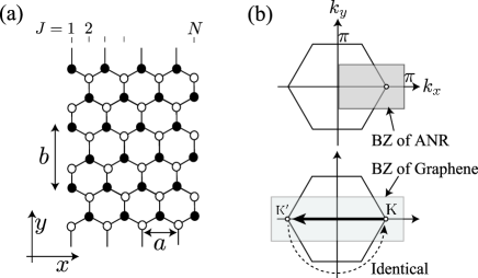
Figure 1: (a) The structure of an ANR. Carbon atoms are divided into A ($\bullet$) and B ($\circ$) atoms. $a$ is a lattice constant [$a=2.46$ Å] and $b\equiv\sqrt{3}a$. (b) Top: BZ of ANR. The point at $(k_{x},k_{y})=(2\pi/3,0)$ is the Dirac point. Bottom: BZ of graphene. The thick arrow denotes the phonon wavevector $(q_{x},q_{y})=(-4\pi/3,0)$ contributing to the first order Raman process in the BZ of ANR, because of zone holding.

The difference between an ANR and graphene appears in their Brillouin zones (BZs). The BZ of an ANR is given by $k_{x}\in(0,\pi)$ and $k_{y}\in[-\pi/2,\pi/2)$ as shown in Fig. 1(b). The BZ of an ANR covers only one half of the graphene’s BZ. Sasaki et al. (2011a) As a result, there is a single Dirac point in the BZ of the ANR, although there are two inequivalent Dirac points (known as K and K^′ points) in the BZ of graphene. Slonczewski and Weiss (1958) The BZ holding for ANRs can be understood more clearly by using the electronic standing wave in ANRs that is written as Sasaki et al. (2011a)

$$\phi^{s}_{\bf k}(x)=\frac{1}{\sqrt{N}}e^{-ik_{y}(J-1)}\sin(k_{x}x)\left(\begin{array}[]{c}e^{-i\Theta({\bf k})}\\ s\end{array}\right),$$ (2)

where $J$ $(=1,\ldots,N)$ denotes the lattice site perpendicular to the edge [Fig. 1(a)], and $x=J$ in units of $a/2=1$. The upper (lower) component of Eq. (2) represents the amplitude at A-atom (B-atom), and the phase $\Theta({\bf k})$ is the polar angle defined with respect to the Dirac point: $k_{y}=(k_{x}-2\pi/3)\tan\Theta({\bf k})$. Because $\Theta({\bf k})$ is invariant throughout the intervalley scattering process at armchair edge, Sasaki et al. (2011a, 2010a); Park et al. (2011) $\phi^{s}_{-k_{x},k_{y}}(x)=-\phi^{s}_{k_{x},k_{y}}(x)$. Thus, $\phi^{s}_{k_{x},k_{y}}(x)$ and $\phi^{s}_{-k_{x},k_{y}}(x)$ are identical, that is, the reflection taking place at armchair edge identifies $(k_{x},k_{y})$ with $(-k_{x},k_{y})$, and one half of the graphene’s BZ needs to be excluded from the BZ of an ANR to avoid a double counting.

The $x$-component of the wavevector, $k_{x}$, is quantized by the boundary condition that is $\phi^{s}_{\bf k}(x)=0$ imposed at $x=0$ and $x=N+1$ (i.e., at fictitious edge sites), as

$$k_{n}=\frac{n\pi}{N+1},\ \ (n=1,\ldots,N),$$ (3)

where $n$ represents the subband index. Note that $k_{n}\in(0,\pi)$ and that the spacing between adjacent $k_{n}$ is $\pi/(N+1)$. This spacing is one half of the spacing obtained by imposing a periodic boundary condition on the wave function, which shows a double density of states in the reduced BZ. The double density of states in the reduced BZ is a direct consequence of the BZ holding and is the principal reason why the energy gap of an ANR is different from that of a (zigzag) nanotube obtained by rolling an ANR into a cylinder. Son et al. (2006) The reduction of the BZ for ANRs is not a matter of notation but a physical result since the energy gap is determined by the double density of states in the reduced BZ. Meanwhile, we assume that $k_{y}$ is a continuous variable. Hereafter we abbreviate $\Theta(k_{n},k_{y})$ and $\phi^{s}_{k_{n},k_{y}}$ by omitting $k_{n}$ and $k_{y}$ as $\Theta_{n}$ and $\phi^{s}_{n}$, respectively.

Due to the BZ holding for ANRs, momentum conservation is relaxed and a phonon with a non-zero wavevector can contribute to a first-order Raman process. For example, an intervalley phonon with a wavevector $(q_{x},q_{y})=(-4\pi/3,0)$ can be excited without disturbing the electronic state since the final electronic state (K^′) is identical to the initial state (K), as shown by the dashed arrow in the lower inset to Fig. 1(b). In graphene without an edge, it is considered that for a photo-excited electron at $(k_{x},k_{y})$, only the phonon at the $\Gamma$ point (${\bf q}=0$) contributes to the first order Raman process due to momentum conservation. Malard et al. (2009) However, in ANRs, a phonon with the wavevector $(q_{x},q_{y})=(-2k_{x},0)$ [mod $\pi$] contributes to the first order Raman process.  As we will show later with the more mathematically rigorous method, the $D$ band is represented as a first order, single resonance process in the reduced BZ, whereas it is commonly recognized as a second order, double resonance process in the BZ of graphene. Thomsen and Reich (2000); Saito et al. (2003)

Vibrational displacement vectors for phonons with ${\bf q}=(q,0)$ in ANRs can be explicitly constructed. First, we define the acoustic and optical branches

$$\sin(qx)\begin{pmatrix}{\bf e}_{i}\cr{\bf e}_{i}\end{pmatrix},\ \ \cos(qx)\begin{pmatrix}{\bf e}_{i}\cr-{\bf e}_{i}\end{pmatrix},$$ (4)

as the basic vibrational modes in ANRs. In Eq. (4), the upper (lower) component represents the vibrational direction of an A-atom (B-atom), where ${\bf e}_{i}$ ($i=x,y$) is the unit vector parallel to the $i$-axis. The function $\sin(qx)$ or $\cos(qx)$ represents the vibrational amplitude of the atom at $x$.  The amplitude may be normalized by multiplying each mode with the proper amplitude $u$. For the optical modes, $u$ is nearly constant at about $0.01$Å, independent of the value of $q$. For the acoustic mode, $u$ depends sensitively on the energy, which is a function of $q$ and temperature. We generally have different amplitudes for acoustic and optical modes. However, at the point $q=2\pi/3$ the energies of the acoustic modes become comparable to that of the optical modes, so the amplitudes of the acoustic and optical modes are approximately the same.  Then normal modes would be given by the sum of the acoustic and optical modes. From the basic vibrational modes given in Eq. (4), we construct new modes as

$${\mbox{\boldmath$u$}}_{q}(x)=\sin(qx)\begin{pmatrix}{\bf e}_{x}\cr{\bf e}_{x}\end{pmatrix}+\cos(qx)\begin{pmatrix}{\bf e}_{y}\cr-{\bf e}_{y}\end{pmatrix}.$$ (5)

This mode is a superposition of the acoustic mode along the $x$-axis (LA) and the optical mode along the $y$-axis (TO). The mode ${\mbox{\boldmath$u$}}_{q}(x)$ with $q=2\pi/3$ corresponds to the Kekulé distortion shown in Fig. 2(a). In Fig. 2(a), it is clear that the Kekulé distortion does not change the bond angle, and that the mode is composed only of a bond stretching motion. Tuinstra and Koenig (1970) The mode ${\mbox{\boldmath$u$}}_{q}(x)$ with $q=0$ can be used to represent the $\Gamma$ point optical mode shown in Fig. 2(b) because the acoustic component in Eq. (5) disappears. We define another combination of acoustic and optical branches as

$${\mbox{\boldmath$v$}}_{q}(x)=\cos(qx)\begin{pmatrix}{\bf e}_{x}\cr-{\bf e}_{x}\end{pmatrix}-\sin(qx)\begin{pmatrix}{\bf e}_{y}\cr{\bf e}_{y}\end{pmatrix}.$$ (6)

This mode is a superposition of the optical mode along the $x$-axis (LO) and the acoustic mode along the $y$-axis (TA). The mode ${\mbox{\boldmath$v$}}_{q}(x)$ is given by a $-90^{\circ}$ rotation of the mode ${\mbox{\boldmath$u$}}_{q}(x)$: $\mbox{\boldmath$v$}_{q}(x)=R(-\pi/2){\mbox{\boldmath$u$}}_{q}(x)$. Thus, the mode ${\mbox{\boldmath$v$}}_{q}(x)$ with $q=2\pi/3$ is realized simply by a change in the bond angle, as shown in 2(c), and the mode ${\mbox{\boldmath$v$}}_{q}(x)$ with $q=0$ is the $\Gamma$ point optical mode shown in Fig. 2(d).

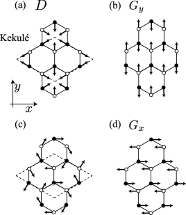
Figure 2: The displacement vectors of four phonon modes. (a) Kekulé distortion $-\mbox{\boldmath$u$}_{2\pi/3}(x)$, (b) $-\mbox{\boldmath$u$}_{0}$ (or $G_{y}$) representing an optical phonon at the $\Gamma$ point, (c) $\mbox{\boldmath$v$}_{2\pi/3}(x)$, and (d) $\mbox{\boldmath$v$}_{0}$ (or $G_{x}$).

According to Tuinstra and Koenig, Tuinstra and Koenig (1970) the $D$ band originates from the Kekulé distortion, while the $G$ band is composed of the two optical components $\mbox{\boldmath$u$}_{0}$ and $\mbox{\boldmath$v$}_{0}$. The vibrational energy of the Kekulé distortion ($\omega^{2}=3K/M$ where $M$ is the mass of the carbon atoms Yoshimori and Kitano (1956)) is highest among the in-plane phonons at the Dirac point, while that for ${\mbox{\boldmath$v$}}_{2\pi/3}$ ($\omega^{2}=18H/M$) is the lowest, because the bond stretching force constant ($K$) is much larger than the force constant for the deformation of the angle ($H$). Tuinstra and Koenig (1970) The $\mbox{\boldmath$u$}_{0}$ and $\mbox{\boldmath$v$}_{0}$ energies are given by $\omega^{2}=3K/M+18H/M$, showing that the $G$ band originates from both bond stretching and bond angle change. Tuinstra and Koenig (1970) Hereafter, we refer to the component of the $G$ band that originates from $\mbox{\boldmath$u$}_{0}$ ($\mbox{\boldmath$v$}_{0}$) as $G_{y}$ ($G_{x}$) band for clarity.

III Electron-phonon interaction

First, we consider the electron-phonon interaction for the vector ${\mbox{\boldmath$u$}}_{q}(x)$. The bond stretching induced by a displacement vector gives rise to two distinct effects: a change in the nearest-neighbor hopping integral and the generation of a (deformation) potential at each atom. The former is known as an off-site interaction and the latter as an on-site interaction. Therefore, the electron-phonon interaction consists of off-site ($H_{\rm off}$) and on-site ($H_{\rm on}$) components. The matrix elements for each component are given by (see Appendix B for derivation)

$$\langle\phi^{s^{\prime}}_{m}|H_{\rm off}({\mbox{\boldmath$u$}}_{q})|\phi^{s}_{n}\rangle=\Bigg{\{} -\left(\frac{2}{N}\sum_{J=1}^{N}\sin(k_{m}J)\cos(qJ)\sin(k_{n}J)\right)\left[2+2\sin\left(\frac{q}{2}+\frac{\pi}{6}\right)\cos\left(\frac{q}{2}\right)\right]$$

$$-\left(\frac{2}{N}\sum_{J=1}^{N}\sin(k_{m}J)\sin(qJ)\cos(k_{n}J)\right)\left[4\sin\left(\frac{q}{2}+\frac{\pi}{6}\right)\sin\left(\frac{q}{2}\right)\sin(k_{n})\right]\Bigg{\}}\langle\sigma_{x}\rangle_{mn}^{s^{\prime}s},$$ (7)

and

$$\langle\phi^{s^{\prime}}_{m}|H_{\rm on}({\mbox{\boldmath$u$}}_{q})|\phi^{s}_{n}\rangle=\left(\frac{2}{N}\sum_{J=1}^{N}\sin(k_{m}J)\cos(qJ)\sin(k_{n}J)\right)\left[4\sin\left(\frac{q}{2}\right)\cos\left(\frac{q}{2}+\frac{\pi}{6}\right)\right]\langle\sigma_{0}\rangle_{mn}^{s^{\prime}s},$$ (8)

where the matrix element of the Pauli matrix $\sigma_{i}$ ($i=x,y,z,0$) is defined as

$$\langle\sigma_{i}\rangle^{s^{\prime}s}_{mn}\equiv\frac{1}{2}\begin{pmatrix}e^{i\Theta_{m}}&s^{\prime}\end{pmatrix}\sigma_{i}\begin{pmatrix}e^{-i\Theta_{n}}\cr s\end{pmatrix},$$ (9)

$\sigma_{0}$ is the 2$\times$2 identity matrix and

$$\sigma_{x}=\begin{pmatrix}0&1\cr 1&0\end{pmatrix},\sigma_{y}=\begin{pmatrix}0&-i\cr i&0\end{pmatrix},\sigma_{z}=\begin{pmatrix}1&0\cr 0&-1\end{pmatrix}.$$ (10)

The right-hand side of the off-site component Eq. (7) is proportional to the pseudospin $\langle\sigma_{x}\rangle_{mn}^{s^{\prime}s}$, while the on-site component depends on $\langle\sigma_{0}\rangle_{mn}^{s^{\prime}s}$. The summations over $J$ in Eq. (7) and Eq. (8), i.e. $(2/N\sum_{J=1}^{N}\ldots)$, do not vanish only when $q$ are specific values that satisfy momentum conservation. So, the matrix element is determined by two factors: pseudospin and momentum conservation.

Let us focus on the first order Raman process, $\phi_{n}^{s}\to\phi_{n}^{s}$ (i.e., $k_{m}=k_{n}$ and $s^{\prime}=s$), that is, the diagonal matrix element in Eq. (7). By executing the summation over $J$ for momentum conservation, we see that the matrix element can be non-zero if the phonon’s wavevector $q$ satisfies (i) $q=0$ or (ii) $q=2\pi-2k_{n}$. The case (i) corresponds to the $\Gamma$ point optical phonon, which is relevant to $G_{y}$, while the case (ii) is relevant to the $D$ band since $q\simeq 2\pi/3$ is satisfied for the electronic states near the Dirac point ($k_{n}\simeq 2\pi/3$).

For the $D$ band, by setting $q\simeq 2\pi/3$ in Eq. (7), we obtain

$$\langle\phi^{s}_{n}|H_{\rm off}({\mbox{\boldmath$u$}}_{q\simeq 2\pi/3})|\phi^{s}_{n}\rangle\simeq 3\langle\sigma_{x}\rangle_{nn}^{ss}.$$ (11)

From Eq. (8), the on-site component almost vanishes $\langle\phi^{s}_{n}|H_{\rm on}({\mbox{\boldmath$u$}}_{q\simeq 2\pi/3})|\phi^{s}_{n}\rangle\simeq 0$, so that only the off-site component contributes to the matrix element. The off-site component is proportional to $\langle\sigma_{x}\rangle_{nn}^{ss}$, which is $s\cos\Theta_{n}$ from Eq. (9). The transition probability $\sim\cos^{2}\Theta_{n}$ takes its maximum (minimum) value when $\Theta_{n}=0$ or $\pi$ ($\Theta_{n}=\pi/2$ or $-\pi/2$). Thus, the electrons at $\Theta_{n}=0$ or $\pi$ contribute selectively to the $D$ band Raman intensity, while the phonon emission from the electrons at $\Theta_{n}=\pi/2$ or $-\pi/2$ is negligible [Fig. 3(a)]. From the wave function Eq. (2), the photo-excited electron at $\Theta=0$ ($\pi$) corresponds to the bonding (antibonding) orbital. This result suggests that the bonding and antibonding orbitals couple strongly to the bond stretching motion, which can be also understood by diagonalizing the 2$\times$2 matrix $H=\gamma\sigma_{x}$ for a two-atom system. The eigenstates of $H$ are bonding or antibonding orbitals. Since the bond stretching motion induces a change in $\gamma$ as $\gamma+\delta\gamma$, the off-site electron-phonon interaction is given by $H_{\rm off}=\delta\gamma\sigma_{x}$, whose expectation values become its maximum for the bonding or antibonding orbitals. Since the $D$ band consists only of the bond stretching motion, the electrons at $\Theta_{n}=0$ and $\pi$ couple strongly to the $D$ band phonon.

For the $G_{y}$ band, by setting $q=0$ in Eq. (7), we obtain

$$\langle\phi^{s}_{n}|H_{\rm off}(\mbox{\boldmath$u$}_{0})|\phi^{s}_{n}\rangle=-3\langle\sigma_{x}\rangle_{nn}^{ss}.$$ (12)

Because there is no contribution from the on-site component [$\langle\phi^{s}_{n}|H_{\rm on}(\mbox{\boldmath$u$}_{0})|\phi^{s}_{n}\rangle=0$ from Eq. (8)], the transition amplitude is determined by the off-site component. It is easy to see that only the electrons at $\Theta_{n}=0$ or $\pi$ contribute to the $G_{y}$ band intensity.

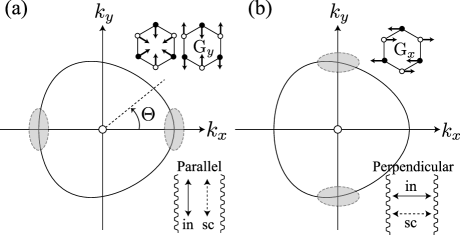
Figure 3: Energy contour circle near the Dirac point. (a) The electrons at the two shaded regions on the energy contour circle ($\Theta\simeq 0$ or $\pi$), have the strongest electron-phonon matrix element for emitting the $D$ and $G_{y}$ bands. These electrons can be selectively excited by the light polarization setup: “in” (“sc”) denotes the polarization of incident (scattered) light. (b) The electrons in the two shaded regions ($\Theta\simeq\pi/2$ or $-\pi/2$), have the strongest electron-phonon matrix element for emitting the $G_{x}$ band.

Comparing Eq. (11) with Eq. (12), we see that the electron-phonon matrix elements for the $D$ and $G_{y}$ bands are the same (apart from the unimportant sign change), although the phonon’s wave vectors are distinct. A direct consequence of this fact is that if the $D$ band is activated, the $G_{y}$ band should be activated in the same manner. For example, the $D$ band intensity at armchair edge becomes comparable to the $G$ band intensity. In addition, due to the fact that both the electron-phonon matrix elements are proportional to $\langle\sigma_{x}\rangle_{nn}^{ss}$, the $D$ and $G_{y}$ band Raman intensities have the same polarization dependence: the Raman intensities of these phonon modes should be enhanced when the polarization of the incident light is parallel to the armchair edge. This polarization dependence of the $D$ band has been confirmed in many experiments. Cançado et al. (2004a); You et al. (2008); Gupta et al. (2009); Casiraghi et al. (2009) Several experimental groups have observed a correlation between the $D$ and $G$ bands, Cançado et al. (2004b); Cong et al. (2010); Begliarbekov et al. (2010); Zhang and Li (2011); Sasaki et al. (2010a) suggesting that the $G_{x}$ Raman intensity is suppressed at the armchair edge. Another example is the correlation between the frequency hardening/softening behavior of the $D$ band due to doping (Kohn anomaly effect) and that of the $G_{y}$ band. These features of the $D$ and $G$ bands are further explored in the following subsections.

Next, we examine the electron-phonon interaction caused by the vector ${\mbox{\boldmath$v$}}_{q}(x)$ defined in Eq. (6). The corresponding electron-phonon matrix element is given by

$$\langle\phi^{s^{\prime}}_{m}|H_{\rm off}({\mbox{\boldmath$v$}}_{q})|\phi^{s}_{n}\rangle=\Bigg{\{} -\left(\frac{2}{N}\sum_{J=1}^{N}\sin(k_{m}J)\sin(qJ)\sin(k_{n}J)\right)\left[2\sin\left(\frac{q}{2}\right)\cos\left(\frac{q}{2}+\frac{\pi}{6}\right)\right]$$

$$-\left(\frac{2}{N}\sum_{J=1}^{N}\sin(k_{m}J)\cos(qJ)\cos(k_{n}J)\right)\left[4\cos\left(\frac{q}{2}\right)\cos\left(\frac{q}{2}+\frac{\pi}{6}\right)\sin(k_{n})\right]\Bigg{\}}i\langle\sigma_{y}\rangle^{s^{\prime}s}_{mn},$$ (13)

and

$$\langle\phi^{s^{\prime}}_{m}|H_{\rm on}({\mbox{\boldmath$v$}}_{q})|\phi^{s}_{n}\rangle=\left(\frac{2}{N}\sum_{J=1}^{N}\sin(k_{m}J)\sin(qJ)\sin(k_{n}J)\right)\left[4\sin\left(\frac{q}{2}\right)\cos\left(\frac{q}{2}+\frac{\pi}{6}\right)\right]\langle\sigma_{z}\rangle^{s^{\prime}s}_{mn}.$$ (14)

A notable difference between the matrix elements for ${\mbox{\boldmath$u$}}_{q}(x)$ and ${\mbox{\boldmath$v$}}_{q}(x)$ is that the off-site components are proportional to $\sigma_{x}$ and $\sigma_{y}$, respectively. Moreover, the on-site interaction induced by ${\mbox{\boldmath$u$}}_{q}(x)$ is symmetric about two sublattices, while that induced by ${\mbox{\boldmath$v$}}_{q}(x)$ is antisymmetric, as is evident from the matrices $\sigma_{0}$ and $\sigma_{z}$ in Eq. (8) and Eq. (14).

From Eq. (14) the on-site component is strongly suppressed for the phonon satisfying $q\simeq 0$ or $q\simeq 2\pi/3$, and it is negligible. For $q\simeq 2\pi/3$, the off-site component is also negligible as $\langle\phi^{s}_{m}|H_{\rm off}({\mbox{\boldmath$v$}}_{q\simeq 2\pi/3})|\phi^{s}_{n}\rangle\simeq 0$ because $\cos(q/2+\pi/6)\simeq 0$ holds. Thus, the mode ${\mbox{\boldmath$v$}}_{q\simeq 2\pi/3}(x)$ does not appear in the Raman spectrum. Since ${\mbox{\boldmath$v$}}_{q\simeq 2\pi/3}(x)$ consists only of a change in bond angle and does not contain any bond stretching motion, the vanishing matrix elements are reasonably understood to show that only the bond stretching motion gives rise to the electron-phonon interaction. For $q\simeq 0$, on the other hand, the off-site component can be non-zero as

$$\langle\phi^{s^{\prime}}_{m}|H_{\rm off}({\mbox{\boldmath$v$}}_{q\simeq 0})|\phi^{s}_{n}\rangle\simeq-\frac{1}{\pi}\left(\frac{1}{m-n+p}+\frac{1}{m-n-p}\right)3i\langle\sigma_{y}\rangle^{s^{\prime}s}_{mn},$$ (15)

where $m-n\pm p$ ($\equiv\Delta n$) is an odd number and integer $p$ is defined through $q=p\pi/(N+1)$. When $m-n\pm p$ is an even number, the off-site element vanishes. The factor $(1/\pi\Delta n)$ on the right-hand side of Eq. (15), originates from momentum conservation, and a small change in the wave number ($m-n\neq 0$) is needed to excite this $G_{x}$ band. A large change in the wave number is not important because the matrix element is suppressed by the inverse of $\Delta n$. By setting $s^{\prime}=s$ and $m\simeq n$ in Eq. (9), we get $\langle\sigma_{y}\rangle_{mn}^{ss}\simeq s\sin\Theta_{n}$. The transition amplitude takes its maximum value when $\Theta_{n}=\pi/2$ or $-\pi/2$. Thus, the electrons at $\Theta_{n}=\pi/2$ or $-\pi/2$ contribute selectively to the $G_{x}$ band Raman intensity, while the phonon emission from the electrons at $\Theta_{n}=0$ or $\pi$ is negligible [Fig. 3(b)]. In the following sections, we point out several consequences that can be derived from the electron-phonon matrix elements.

III.1 $D$ band splitting

The fact that there are the two electronic states with bonding or antibonding orbitals ($\Theta=0$ or $\pi$) from which the $D$ band phonon is emitted results in the splitting of the $D$ band if we take account of the trigonal warping effect. The splitting width increases with increasing incident laser energy $E_{L}$ as

$$\Delta\omega_{D}=25\left(\frac{E_{L}}{\gamma}\right)^{2}\ [{\rm cm}^{-1}],$$ (16)

which is about 15 cm^-1 when $E_{L}=2.3$ eV. This formula is derived as follows.

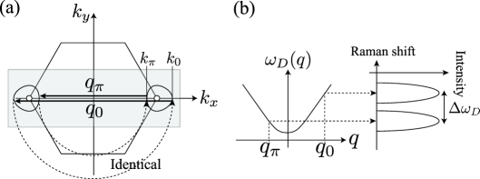
Figure 4: (a) Two principal wavevectors of the phonons ($q_{0}$ and $q_{\pi}$) contributing to the $D$ band. (b) The phonon dispersion relation near the Dirac point. The energy difference between $\omega_{D}(q_{0})$ and $\omega_{D}(q_{\pi})$ appears as two peaks in the $D$ band.

Since the probability that the photo-excited electron at $\Theta$ emits the Kekulé mode is proportional to $\cos^{2}\Theta$ [Eq. (11)], the photo-excited electrons satisfying $\Theta\simeq 0$ or $\Theta\simeq\pi$, indicated by the shaded regions shown in Fig. 3(a), contribute efficiently to the $D$ band intensity. Thus, two phonon modes that originate from the two regions in the photo-excited electron contribute to the $D$ band. We denote $k_{x}$ at $\Theta=0$ ($\Theta=\pi$) as $k_{0}$ ($k_{\pi}$) [see Fig. 4(a)], where $k_{0}$ and $k_{\pi}$ are given by solving the equation $E_{L}/2=\gamma|1+2\cos(k_{x})|$ as

$$\begin{split}&k_{0}-\frac{2\pi}{3}=\frac{\sqrt{3}}{2}\left(\frac{E_{L}}{3\gamma}\right)+\frac{\sqrt{3}}{8}\left(\frac{E_{L}}{3\gamma}\right)^{2}+\cdots,\\ &\frac{2\pi}{3}-k_{\pi}=\frac{\sqrt{3}}{2}\left(\frac{E_{L}}{3\gamma}\right)-\frac{\sqrt{3}}{8}\left(\frac{E_{L}}{3\gamma}\right)^{2}+\cdots.\end{split}$$ (17)

The $\pm$ signs in front of $\sqrt{3}/8(E_{L}/3\gamma)^{2}$ represent the trigonal warping effect meaning that the energy contour circle is anisotropic as shown in Figs. 3 and 4(a). The corresponding phonon’s wavevector is given by $q_{0/\pi}=2\pi-2k_{0/\pi}$ [Fig. 4(a)]. Then we find that the difference between the phonon’s wavevectors $|q_{0}-2\pi/3|$ (relative to the Dirac point) and $|q_{\pi}-2\pi/3|$ is well approximated by

$$\Delta q=\frac{\sqrt{3}}{2}\left(\frac{E_{L}}{3\gamma}\right)^{2}.$$ (18)

For simplicity, let us assume that the phonon dispersion relation for the $D$ band is isotropic about the Dirac point: $\omega_{D}$ is a function of $|q-2\pi/3|$ as $\omega_{D}(|q-2\pi/3|)$. From Fig. 4(b) it is clear that the two phonon modes with $q_{0}$ and $q_{\pi}$ have different phonon energies, which results in the double peak structure of the $D$ band.

The difference between the energy for the phonon mode with $q_{0}$ and that for $q_{\pi}$ is approximated by

$$\Delta\omega_{D}=\frac{\partial\omega_{D}}{\partial q}\Delta q,$$ (19)

where $\partial\omega_{D}/\partial q$ is the slope of the phonon energy dispersion. The value of the slope can be estimated from the dispersive behavior of the $D$ band: the $D$ band frequency increases as the laser energy $E_{L}$ increases. For example, Matthews et al. Matthews et al. (1999) reported that $\partial\omega_{D}/\partial E_{L}$ for graphite is about 50 cm${}^{-1}/$eV. A similar value has been obtained for single layer graphene. Gupta et al. (2009); Casiraghi et al. (2009) We interpret the dispersive behavior that occurs as a result of the dispersion relation of the phonon mode. Matthews et al. (1999) Then we have

$$\frac{\partial\omega_{D}}{\partial E_{L}}=\frac{\partial q}{\partial E_{L}}\frac{\partial\omega_{D}}{\partial q}.$$ (20)

By combining $E_{L}/2=\gamma|1+2\cos(k)|$ and $q=2\pi-2k$, we have $|\partial E_{L}/\partial q|\approx\sqrt{3}\gamma$ for the states near the Dirac point. Putting this result in Eq. (20), we have $\partial\omega_{D}/\partial q=\sqrt{3}\gamma(\partial\omega_{D}/\partial E_{L})$. Then we obtain Eq. (16) by combining Eq. (18) and Eq. (19). Actual splitting can be smaller (or even larger) than Eq. (16) due to several factors, such as (i) the phonon dispersion relation for the $D$ band not being exactly isotropic around the Dirac point, (ii) $\Theta$ is not exactly limited by $0$ or $\pi$. The conditions for observing the splitting are discussed later.

III.2 Light polarization dependence

Pseudospin is the key to the characteristic polarization dependence of the $D$ and $G$ band intensities. Below we show that the Raman intensities are enhanced only when the polarizations of the incident and scattered light are both parallel to the armchair edge. That is, the $D$ band intensity is well approximated by

$$I_{\rm D}(\Theta_{\rm in},\Theta_{\rm sc})\simeq I\cos^{2}(\Theta_{\rm in})\cos^{2}(\Theta_{\rm sc}),$$ (21)

where $\Theta_{\rm in}$ ($\Theta_{\rm sc}$) the angle between the orientation of the armchair edge and the incident (scattered) light polarization. Sasaki et al. (2010b) Without a polarizer for the scattered light, we obtain $I_{\rm D}(\Theta_{\rm in})\simeq I\pi\cos^{2}(\Theta_{\rm in})$ by integrating $I_{\rm D}(\Theta_{\rm in},\Theta_{\rm sc})$ over $\Theta_{\rm sc}$.

To discuss light polarization dependence, let us review the interband optical matrix elements obtained in a previous paper. Sasaki et al. (2011b) The electron-light interaction is written as $H(\mbox{\boldmath$\epsilon$})=-e\mbox{\boldmath$v$}\cdot{\bf A}$, where $-e$ is the electron charge, $\mbox{\boldmath$v$}=(v_{x},v_{y})$ is the velocity operator, and ${\bf A}=A\mbox{\boldmath$\epsilon$}e^{-i\omega t}$ is a spatially uniform vector potential. Here, $\hbar\omega$ corresponds to the incident light energy and $\epsilon$ denotes the polarization. The calculated matrix elements are given in units of $-ev_{\rm F}A$ by

$$\langle\phi^{c}_{m}|H(\epsilon_{x})|\phi^{v}_{n}\rangle=\begin{cases}\displaystyle 0&\text{$m-n\in$ even},\\ \displaystyle-\frac{2}{\pi}\frac{\langle\sigma_{y}\rangle_{mn}^{cc}}{m-n}&\text{$m-n\in$ odd},\end{cases}$$ (22)

$$\langle\phi^{c}_{m}|H(\epsilon_{y})|\phi^{v}_{n}\rangle=i\delta_{mn}\langle\sigma_{x}\rangle_{mn}^{cc}.$$ (23)

The Kronecker delta $\delta_{mn}$ in Eq. (23) shows that the $y$-polarized light ($\epsilon_{y}$: parallel to the armchair edge) results in a direct interband transition ($m=n$). The transition amplitude depends on the diagonal matrix element of the pseudospin $\langle\sigma_{x}\rangle_{nn}^{cc}$. As we have seen, $|\langle\sigma_{x}\rangle^{cc}_{nn}|$ takes its maximum value for $\Theta_{n}=0$ or $\pi$. On the other hand, $|\langle\sigma_{x}\rangle_{nn}^{cc}|$ vanishes for $\Theta_{n}=\pm\pi/2$. Therefore, only the electrons at $\Theta_{n}=0$ or $\pi$ are selectively excited by the $y$-polarized light. From Eq. (22), the $x$-polarized light ($\epsilon_{x}$: perpendicular to the edge) results in an indirect interband transition ($m-n=\pm 1,\pm 3,\ldots$), and the optical transition probability is reduced by the factor of $(2/\pi)^{2}(m-n)^{-2}$, independent of the pseudospin $\langle\sigma_{y}\rangle_{mn}^{cc}$.

First, we consider a parallel configuration: both the incident and scattered lights are $y$-polarized [see Fig. 3(a)]. Since the absorption and emission of $y$-polarized light occur through direct transitions $\phi_{n}^{v}\leftrightarrow\phi_{n}^{c}$, the phonon mode with $q=0$ or $q=2\pi-2k_{n}$ fulfils the momentum conservation of the first order Raman process. Thus, the $D$ and $G_{y}$ bands can be detected by the parallel configuration. The $G_{x}$ band is suppressed because its activation requires a non-zero shift in the electron wave number, and the momentum deficit cannot be compensated by direct optical transitions. More importantly, pseudospin enhances (suppresses) the Raman intensities of the $D$ and $G_{y}$ bands ($G_{x}$ band) because the probability amplitude of exciting the $D$ and $G_{y}$ bands ($G_{x}$ band) is proportional to $\cos\Theta_{n}$ ($\sin\Theta_{n}$). The function $\cos\Theta_{n}$ agrees with the optical matrix element that is also proportional to $\cos\Theta_{n}$, while the function $\sin\Theta_{n}$ is out-of-phase. The probability that the electron at $\Theta_{n}$ completes the Raman process by emitting the D or $G_{y}$ band ($G_{x}$ band) is proportional to $\cos^{6}\Theta_{n}$ ($\cos^{4}\Theta_{n}\sin^{2}\Theta_{n}$). We estimate the reduction in the intensity of the $G_{x}$ band caused by the disagreement of the pseudospin to be 1/5 by using the ratio of $\oint\cos^{4}\Theta_{n}\sin^{2}\Theta_{n}d\Theta_{n}$ ($=\pi/8$) to $\oint\cos^{6}\Theta_{n}d\Theta_{n}$ ($=5\pi/8$). The $G_{x}$ band intensity is further reduced by the momentum deficit.

Next, we examine a crossed configuration: the incident light is $y$-polarized, while the scattered light is $x$-polarized. Since $x$($y$)-polarized light results in an indirect (direct) optical transition, momentum mismatch takes place: the electron cannot return to its original state in the valence band unless a phonon with a specific momentum is involved in the Raman process. The intensity is suppressed by a factor of $(2/\pi)^{2}$ because of the reduction factor in the optical matrix element for the $x$-polarized light. Furthermore, momentum conservation for the phonon mode reduces the emission probability by the factor of $(2/\pi)^{2}$ for the $G_{x}$ band [or $(1/2)^{2}$ for the $D$ and $G_{y}$ bands], so that the intensity is suppressed by a factor of $(2/\pi)^{4}$ ($\simeq 0.16$). Moreover, the pseudospin for incident light does not match that for scattered light, and the Raman intensity is suppressed by a factor of $1/5$ in the crossed configuration. Thus, the $D$ and $G_{y}$ bands intensities are suppressed by a few percent compared with the intensities in the parallel configuration.

Finally, we study a perpendicular configuration: both the incident and scattered lights are $x$-polarized [see Fig. 3(b)]. The Raman intensities of the $D$, $G_{y}$, and $G_{x}$ bands for this configuration are suppressed by $(2/\pi)^{4}$ at least, due to the reduction factor for the optical matrix elements. The pseudospin for the $x$-polarized light agrees only with that for the $G_{x}$ band. Thus, the $D$ and $G_{y}$ bands are not detectable in the perpendicular configuration because of the further reduction by a factor of $1/5$.

When the polarization of the incident light is perpendicular to the armchair edge, it is common for the $D$ band to show a residual intensity. Cançado et al. (2004a); Casiraghi et al. (2009); Gupta et al. (2009); Cong et al. (2010) The ratio of the minimum $D$ band intensity (observed when the incident light polarization is perpendicular to the edge) to the maximum intensity (observed when the incident light polarization is parallel to the edge) is 0.12 $\sim$ 0.2 depending on the experiments. Several authors have suggested that the presence of the residual $D$ band intensity is correlated with the irregularities that consist of armchair segments having angles of $\pm 60^{\circ}$ with respect to the armchair edge. Cançado et al. (2004a); Casiraghi et al. (2009); Xu et al. (2011) Because their arguments assume that the irregularities contribute independently to the total $D$ band intensity as $I_{\rm D}(\Theta_{\rm in})\simeq a\cos^{2}(\Theta_{\rm in})+b\{\cos^{2}(\Theta_{\rm in}+60^{\circ})+\cos^{2}(\Theta_{\rm in}-60^{\circ})\}$, there is a possibility that this assumption is not plausible when the electron wave function extends along the armchair edge. We provide a different interpretation of the residual $D$ band intensity. When the momentum conservation that we have used is not physically legitimate because of the boundary condition of the phonon mode (see Appendix B for a relevant discussion), we can only rely on the pseudospin. Then we may expect the residual $D$ band intensity to be about $0.2$ ($1/5$). Even for an armchair edge without irregularity, the $D$ band exhibits a residual intensity depending on the boundary condition of the phonon mode.

Without a polarizer for the scattered light, the $D$ band polarization dependence is expressed as

$$I_{\rm D}(\Theta_{\rm in})=a\cos^{2}(\Theta_{\rm in})+b\sin^{2}(\Theta_{\rm in})+c,$$ (24)

where $a$, $b$, and $c$ are parameters. When both the momentum conservation and pseudospin are physically legitimate, $b\simeq 0$. When we can only rely on the pseudospin, we expect $b/a$ to be 1/3 by using the ratio of $\oint\cos^{2}\Theta\sin^{2}\Theta d\Theta$ ($=\pi/4$) to $\oint\cos^{4}\Theta d\Theta$ ($=3\pi/4$). Figure 5 shows the polar plots for these two cases. If the residual $D$ band intensity decreases by putting a polarizer for the scattered light, such a signal would evidence the effect of the pseudospin. The $\Theta_{\rm in}$ independent $c$ term may originate from a point defect or on-site deformation potential (see Appendix A) and obscures the $D$ band polarization dependence.

Figure 5: The polar plot for the $D$ band intensity. The parameters for the solid curve are $a=1$, $b=1/3$, and $c=0$, while those for the dashed curve are $a=1$ and $b=c=0$.

III.3 Kohn anomaly and transport

In ANRs, because of the conical shape of the energy spectrum, momentum conservation tells us that a vertical (direct) electron-hole pair can couple to the $\Gamma$ point phonon. Furthermore, due to the BZ holding, the direct electron-hole pair can also couple to the $D$ band phonons. As a result, the G and $D$ bands in Raman spectra can exhibit a similar Kohn anomaly effect. The probability amplitude for the process whereby the $D$ and $G_{y}$ bands change into a vertical electron-hole pair is given by using $|\phi^{v}_{n}\rangle=\sigma_{z}|\phi^{c}_{n}\rangle$, $\sigma_{x}\sigma_{z}=-i\sigma_{y}$, Eq. (11), and Eq. (12), as

$$\begin{split}&\langle\phi^{c}_{n}|H_{\rm off}({\mbox{\boldmath$u$}}_{q\simeq 2\pi/3})|\phi^{v}_{n}\rangle=-3i\langle\sigma_{y}\rangle^{cc}_{nn},\\ &\langle\phi^{c}_{n}|H_{\rm off}(\mbox{\boldmath$u$}_{0})|\phi^{v}_{n}\rangle=3i\langle\sigma_{y}\rangle^{cc}_{nn}.\end{split}$$ (25)

Since $\langle\sigma_{y}\rangle^{cc}_{nn}=\sin\Theta_{n}$, electrons at $\Theta_{n}=\pi/2$ or $-\pi/2$ contribute to the Kohn anomaly. Equation (25) clearly shows that the behavior of the Kohn anomaly for the $D$ band is correlated to that for the $G_{y}$ band: if the $D$ band exhibits hardening/softening due to the Kohn anomaly effect, the $G_{y}$ band also exhibits hardening/softening. Recently, Zhang and Li Zhang and Li (2011) have observed a Kohn anomaly effect for the G band at an armchair graphene edge. Interestingly they also found a correlation between the 2$D$ band and the $G$ band.

It is interesting to note that the pseudospin for electron-hole pair creation is identical to the matrix elements of the velocity operator along the armchair edge, which is written as $\langle\phi^{c}_{m}|v_{y}|\phi^{c}_{n}\rangle=\delta_{mn}v_{\rm F}\langle\sigma_{y}\rangle_{mn}^{cc}$. Sasaki et al. (2011b) Thus, the Kohn anomaly effect is fundamentally related to the velocity or current behavior. If the velocity is suppressed, then the Kohn anomaly effect is suppressed as well. The velocity perpendicular to the armchair edge $v_{x}$ is suppressed by electron reflection, while the velocity along the edge $v_{y}$ is not. As a result, only the $D$ and $G_{y}$ bands can experience a strong Kohn anomaly effect. Sasaki et al. (2010b) In the presence of impurities, the electronic velocity (current) along the edge (ribbon) might also be suppressed due to the scattering. However, in metallic ANR, because Berry’s phase can protect the electronic current along the armchair edge from decaying, Sasaki et al. (2010c) the Kohn anomaly effect for the $D$ and $G_{y}$ bands should be robust against impurity potentials. We consider that the $D$ and $G_{y}$ bands undergo a strong Kohn anomaly effect even when we take account of the effect of impurity potentials.

IV Discussion

Here we discuss the possible factors that obscure the double-component feature of the $D$ band proposed in Sec. III.1. First, the resonance effect suppresses the intensity of one of the two components. Suppose that the electron at $k_{0}$ is resonant with the incident laser energy. Then the Raman intensity for the process in which the photo-excited electron at $k_{0}$ emits a phonon with momentum $q_{0}$ is enhanced as compared with the Raman intensity involving a phonon with momentum $q_{\pi}$. Such a resonance effect is apparent in thin ANRs, whereas it is negligible for thick ANRs if the ANR width (W) exceeds a critical value. The critical $W$ is estimated from the condition whereby the difference between $k_{0}-2\pi/3$ and $2\pi/3-k_{\pi}$ caused by the trigonal warping effect [Eq. (17)] is larger than the spacing of each sub-band, $\pi/(N+1)$. This condition leads to $W>8(\gamma/E_{L})^{2}$ nm: $W>13$ nm when $E_{L}=2.3$ eV. Second, for thick ANRs satisfying $W>8(\gamma/E_{L})^{2}$ nm or for armchair edges of graphene, the energy gap is smaller than the energy of the $D$ band. As a result, the width of each peak can be wide enough to obscure the splitting structure since the $D$ band undergoes a strong Kohn anomaly effect (Sec. III.3). To suppress the broadening of each peak caused by the Kohn anomaly effect, the Fermi energy needs to be placed away from the Dirac point ($|E_{\rm F}|>0.1$ eV). Third, the parallel configuration is the most suitable polarization setting with which to observe the splitting of the $D$ band because the probability $\cos^{6}\Theta$ exhibits prominent peaks at $\Theta=0$ or $\pi$. To observe the splitting of the $D$ band, it is important to recognize that the results obtained in Secs. III.1, III.2, and III.3 are closely correlated. Among the conclusions obtained in Secs. III.1, III.2, and III.3, we think that the light polarization dependence of the $D$ band Raman intensity is the most direct conclusion derived from the pseudospins of the electron-phonon and optical matrix elements. Indeed, many studies have reported the $D$ band polarization behavior. Cançado et al. (2004a); You et al. (2008); Gupta et al. (2009); Casiraghi et al. (2009); Cong et al. (2010); Barros et al. (2011) However, there is a small possibility that only the pseudospin of the optical matrix element is the result of the observed polarization dependence for the $D$ band if there is a strong resonance effect.  A strong piece of evidence for the pseudospin of the electron-phonon matrix element is provided by the splitting of the $D$ band.

A multicomponent $D$ band has been seen in several sets of Raman data obtained at the graphene edge. Ferrari et al. Ferrari et al. (2006) and Gupta et al. Gupta et al. (2009) reported that for graphite, the $D$ band can be well fitted by a doublet with two broad components, although a single-layer graphene edge produces a narrow single-component $D$ band. Our theory relates to the armchair edge of a single-layer graphene. However, the results that we have obtained for ANRs may be applicable to single-wall carbon nanotubes because defects in carbon nanotubes result in the formation of a standing wave. Suzuki and Hibino Suzuki and Hibino (2011) reported that there is a correlation between the behaviors of the $D$ and $G$ bands under doping. Moreover, they observed $D$ band splitting when the excitation laser energy was at its largest (532 nm), while such a splitting was not seen when they used lower excitation energies, 633 nm and 785 nm. These observations are consistent with our results, that is, Kohn anomaly effects for the $D$ and $G$ bands are correlated and the $D$ band splitting increases with increasing $E_{L}$. We note that work has already been published on the splitting of the $D$ band in carbon nanotubes, Maultzsch et al. (2001); Zólyomi et al. (2003) in which the authors propose a completely different mechanism from ours (trigonal warping effect for phonon dispersion).

V Conclusion

By constructing the matrix element of the electron-phonon interaction for the $D$ band analytically, we have shown that the $D$ band in an ANR is represented as a first order, single resonance process in a reduced BZ, as well as the $G$ band. This explains clearly and naturally the fact that the $D$ and $G$ bands show a similar intensity in many experiments for armchair edge. The matrix element is proportional to the pseudospin $\langle\sigma_{x}\rangle_{nn}^{cc}$, and the $D$ band couples selectively to the two pseudospin states $\langle\sigma_{x}\rangle_{nn}^{cc}=\pm 1$ corresponding to the bonding and antibonding orbitals. The pseudospin is the origin of the branches of phenomena associated with the $D$ band in ANRs, as shown in Secs. III.1, III.2, and III.3. The polarization dependence of the $D$ band is consistent with the previous experimental reports. Direct evidence for the pseudospin of the $D$ band is provided by the $D$ band splitting at the armchair edge, which has not been previously reported.

Appendix A Generalized Kekulé distortion

When the amplitudes of the acoustic and optical modes are not exactly the same, we may consider the extension of Eq. (4) to the general case as

$$(1-\epsilon)\sin(qx)\begin{pmatrix}{\bf e}_{x}\cr{\bf e}_{x}\end{pmatrix}+(1+\epsilon)\cos(qx)\begin{pmatrix}{\bf e}_{y}\cr-{\bf e}_{y}\end{pmatrix}.$$ (26)

In this Appendix, we show how the analysis is affected by the deviation $\epsilon$.

The generalized displacement vector is written as ${\mbox{\boldmath$u$}}_{q}(x)+\epsilon{\mbox{\boldmath$u$}}_{-q}(x)$, and the corresponding electron-phonon matrix elements are

$$\langle\phi^{s^{\prime}}_{m}|H_{\rm on/off}({\mbox{\boldmath$u$}}_{q}+\epsilon{\mbox{\boldmath$u$}}_{-q}))|\phi^{s}_{n}\rangle=\langle\phi^{s^{\prime}}_{m}|H_{\rm on/off}({\mbox{\boldmath$u$}}_{q})|\phi^{s}_{n}\rangle+\epsilon\langle\phi^{s^{\prime}}_{m}|H_{\rm on/off}({\mbox{\boldmath$u$}}_{-q})|\phi^{s}_{n}\rangle.$$ (27)

Because the last term is given by replacing $q$ with $-q$ in Eqs. (7) and (8), we see that the off-site component is suppressed for $q\simeq 2\pi/3$, $\epsilon\langle\phi^{s^{\prime}}_{m}|H_{\rm off}({\mbox{\boldmath$u$}}_{-q\simeq-\frac{2\pi}{3}})|\phi^{s}_{n}\rangle\simeq 0$, and that the correction to the matrix element of Eq. (11) arises only from the on-site component, $\epsilon\langle\phi^{s^{\prime}}_{m}|H_{\rm on}({\mbox{\boldmath$u$}}_{-q\simeq-\frac{2\pi}{3}})|\phi^{s}_{n}\rangle\simeq-3\epsilon\langle\sigma_{0}\rangle_{mn}^{s^{\prime}s}$. Thus, the total electron-phonon matrix element for the deformed Kekulé distortion is given by

$$3g_{\rm off}\langle\sigma_{x}\rangle_{mn}^{s^{\prime}s}-3\epsilon g_{\rm on}\langle\sigma_{0}\rangle_{mn}^{s^{\prime}s},$$ (28)

where $g_{\rm on}$ ($g_{\rm off}$) denotes the coupling constant of the on-site (off-site) deformation potential. Since the intensity is relevant to the square of the matrix element, the correction can include the crossing term $-18\epsilon g_{\rm on}g_{\rm off}\langle\sigma_{x}\rangle_{nn}^{ss}\langle\sigma_{0}\rangle_{nn}^{ss}$ and the order $\epsilon^{2}$ term $9\epsilon^{2}g^{2}_{\rm on}(\langle\sigma_{0}\rangle_{nn}^{ss})^{2}$. The crossing term does not contribute to the intensity because it vanishes after the integral over $\Theta_{n}$. Thus, the leading contribution is given by the order $\epsilon^{2}$. The effect of the deviation is negligible when $|\epsilon|\ll|g_{\rm off}/g_{\rm on}|$, where $|g_{\rm off}/g_{\rm on}|\sim 1/3$ was suggested by the result of density functional theory. Porezag et al. (1995) Note also that the pseudospin is proportional to $\sigma_{0}$, which shows that the deviation is not relevant to the polarization dependence of the $D$ band intensity but relevant to the $c$ parameter in Eq. (24) or residual $D$ band intensity.

Using Eq. (28), a quick comparison can be made between the predictions of our model on which the $D$ band is described as coming from a Kekulé distortion and other models where the $D$ band is described solely as a combination of intervalley optical phonons. The consequence of other models may be obtained by setting $\epsilon=1$ in Eq. (28). Then, the matrix element is dominated by the on-site component and the pseudospin $\sigma_{x}$ is suppressed. As a result, the $D$ band does not exhibit the polarization dependence.

Appendix B Derivations of Eqs. (7) and (8), and boundary condition for phonon

Below we give the derivation of the electron-phonon matrix elements. Note that $\mbox{\boldmath$u$}_{q}(J)$ in Eq. (5) consists only of the optical mode at the fictitious edge site of $J=0$. This means that Eq. (5) results from a specific choice of phonon boundary condition. To make the derivation general enough to cover the possible boundary conditions, we first generalize $\mbox{\boldmath$u$}_{q}(J)$ of Eq. (5) by inserting a phase shift of $\varphi$ as

$$\sin(qJ+\varphi)\begin{pmatrix}{\bf e}_{x}\cr{\bf e}_{x}\end{pmatrix}+\cos(qJ+\varphi)\begin{pmatrix}{\bf e}_{y}\cr-{\bf e}_{y}\end{pmatrix}.$$ (29)

For $\varphi=0$, Eq. (29) reproduces Eq. (5). For $\varphi=\pi/2$, Eq. (29) leads to

$$\bar{\mbox{\boldmath$u$}}_{q}(J)=\cos(qJ)\begin{pmatrix}{\bf e}_{x}\cr{\bf e}_{x}\end{pmatrix}-\sin(qJ)\begin{pmatrix}{\bf e}_{y}\cr-{\bf e}_{y}\end{pmatrix}.$$ (30)

This $\bar{\mbox{\boldmath$u$}}_{q}(J)$ consists only of the acoustic mode at $J=0$, which is contrasted with that $\mbox{\boldmath$u$}_{q}(J)$ of Eq. (5) that consists only of the optical mode at $J=0$.  The phase $\varphi$ is not very meaningful for a periodic system without an edge, such as a nanotube, however, for a nanoribbon with an edge, phase $\varphi$ should be taken into account because it is possible that the phonon boundary condition could be sensitive to the situation of the armchair edge. It turns out that $\varphi$ changes the momentum conservation slightly, while it does not modify the pseudospin structure of the matrix element. Thus, an analysis based on the pseudospin seems plausible, while the results based only on the momentum conservation might be physically fragile. Similarly, the $\mbox{\boldmath$v$}_{q}(J)$ mode can be generalized as

$$\cos(qJ+\varphi)\begin{pmatrix}{\bf e}_{x}\cr-{\bf e}_{x}\end{pmatrix}-\sin(qJ+\varphi)\begin{pmatrix}{\bf e}_{y}\cr{\bf e}_{y}\end{pmatrix}.$$ (31)

In addition, the physics of graphene edge is, in some sense, an understanding of the boundary conditions at edges. The importance of the boundary conditions for electrons has been widely recognized, while those for the phonon mode and for electron-phonon interactions are yet to be understood.

The off-site electron-phonon matrix elements for the displacement vector ${\mbox{\boldmath$u$}}_{q}(J)$ of Eq. (29) are written as

$$\langle\phi^{s^{\prime}}_{m}|H_{\rm off}({\mbox{\boldmath$u$}}_{q})|\phi^{s}_{n}\rangle=\sum_{J=1}^{N}\left[\phi^{s^{\prime}}_{m,J}\right]^{\dagger}\left(\delta h^{+}_{J}G^{+}\phi^{s}_{n,J+1}+\delta h_{J}\phi^{s}_{n,J}+\delta h_{J}^{-}G^{-}\phi^{s}_{n,J-1}\right).$$ (32)

On the right-hand side, we have defined the translational operators,

$$G^{+}\equiv\begin{pmatrix}e^{ik_{y}b}&0\cr 0&1\end{pmatrix},\ \ G^{-}\equiv\begin{pmatrix}1&0\cr 0&e^{-ik_{y}b}\end{pmatrix},$$ (33)

and the 2$\times$2 matrices of the deformation potential as

$$\begin{split}&\delta h_{J}=\begin{pmatrix}0&\delta\gamma_{1}(J)\cr\delta\gamma_{1}(J)&0\end{pmatrix},\\ &\delta h_{J}^{+}=\begin{pmatrix}0&\delta\gamma_{3}(J)\cr\delta\gamma_{2}(J+1)&0\end{pmatrix},\\ &\delta h_{J}^{-}=\begin{pmatrix}0&\delta\gamma_{2}(J)\cr\gamma_{3}(J-1)&0\end{pmatrix},\end{split}$$ (34)

where

$$\begin{split}&\delta\gamma_{1}(J)=\left[{\mbox{\boldmath$u$}}_{q}^{\rm B}(J)-{\mbox{\boldmath$u$}}_{q}^{\rm A}(J)\right]\cdot{\bf e}_{1},\\ &\delta\gamma_{2}(J)=\left[{\mbox{\boldmath$u$}}_{q}^{\rm B}(J-1)-{\mbox{\boldmath$u$}}_{q}^{\rm A}(J)\right]\cdot{\bf e}_{2},\\ &\delta\gamma_{3}(J)=\left[{\mbox{\boldmath$u$}}_{q}^{\rm B}(J+1)-{\mbox{\boldmath$u$}}_{q}^{\rm A}(J)\right]\cdot{\bf e}_{3},\end{split}$$ (35)

with ${\mbox{\boldmath$u$}}_{q}^{\rm A}(J)=\sin(qJ+\varphi){\bf e}_{x}+\cos(qJ+\varphi){\bf e}_{y}$ and ${\mbox{\boldmath$u$}}_{q}^{\rm B}(J)=\sin(qJ+\varphi){\bf e}_{x}-\cos(qJ+\varphi){\bf e}_{y}$ from 29. In Eq. (35) ${\bf e}_{a}$ ($a=1,2,3$) are the dimensionless unit vectors pointing from an A-atom to the nearest-neighbor B-atoms:

$${\bf e}_{1}={\bf e}_{y},{\bf e}_{2}=-\frac{\sqrt{3}}{2}{\bf e}_{x}-\frac{1}{2}{\bf e}_{y},{\bf e}_{3}=\frac{\sqrt{3}}{2}{\bf e}_{x}-\frac{1}{2}{\bf e}_{y}.$$ (36)

By inserting Eq. (29) into Eq. (35), we rewrite Eq. (34) as

$$\begin{split}&\delta h_{J}=-2\sigma_{x}\cos(qJ+\varphi),\\ &\delta h_{J}^{+}=2\sigma_{x}\cos\left(qJ+\varphi+\frac{q}{2}\right){\bf e}_{q}\cdot{\bf e}_{3},\\ &\delta h_{J}^{-}=2\sigma_{x}\cos\left(qJ+\varphi-\frac{q}{2}\right){\bf e}_{q}\cdot{\bf e}_{3},\end{split}$$ (37)

where we have defined

$${\bf e}_{q}=\sin\left(\frac{q}{2}\right){\bf e}_{x}-\cos\left(\frac{q}{2}\right){\bf e}_{y}.$$ (38)

It is easy to show that ${\bf e}_{q}$ satisfies

$${\bf e}_{q}\cdot{\bf e}_{3}=\sin\left(\frac{q}{2}+\frac{\pi}{6}\right)={\bf e}_{-q}\cdot{\bf e}_{2}.$$ (39)

Finally, by putting Eq. (37) into Eq. (32), we obtain

$$\langle\phi^{s^{\prime}}_{m}|H_{\rm off}({\mbox{\boldmath$u$}}_{q})|\phi^{s}_{n}\rangle$$

$$= \sum_{J=1}^{N}\left[\phi^{s^{\prime}}_{m,J}\right]^{\dagger}\left\{2T{\bf e}_{q}\cdot{\bf e}_{3}\cos\left(qJ+\varphi+\frac{q}{2}\right)\phi^{s}_{n,J+1}-2\sigma_{x}\cos\left(qJ+\varphi\right)\phi^{s}_{n,J}+2T^{-1}{\bf e}_{q}\cdot{\bf e}_{3}\cos\left(qJ+\varphi-\frac{q}{2}\right)\phi^{s}_{n,J-1}\right\}$$

$$= \sum_{J=1}^{N}\left[\phi^{s^{\prime}}_{m,J}\right]^{\dagger}\left\{-2\cos(qJ+\varphi)\left[\sigma_{x}+K_{n}^{s}{\bf e}_{q}\cdot{\bf e}_{3}\cos\left(\frac{q}{2}\right)\right]\phi^{s}_{n,J}-2\sin(qJ+\varphi){\bf e}_{q}\cdot{\bf e}_{3}\sin\left(\frac{q}{2}\right)\left[T\phi^{s}_{n,J+1}-T^{-1}\phi^{s}_{n,J-1}\right]\right\}$$

$$= \Bigg{\{}-\left(\frac{2}{N}\sum_{J=1}^{N}\sin(k_{m}J)\cos(qJ+\varphi)\sin(k_{n}J)\right)\left[2+2{\bf e}_{q}\cdot{\bf e}_{3}\cos\left(\frac{q}{2}\right)\right]$$

$$\ \ \ -\left(\frac{2}{N}\sum_{J=1}^{N}\sin(k_{m}J)\sin(qJ+\varphi)\cos(k_{n}J)\right)\left[4{\bf e}_{q}\cdot{\bf e}_{3}\sin\left(\frac{q}{2}\right)\sin(k_{n})\right]\Bigg{\}}\langle\sigma_{x}\rangle^{s^{\prime}s}_{mn},$$ (40)

where the matrix $T$ ($T^{-1}$) is defined by $T\equiv\sigma_{x}G^{+}$ ($T^{-1}\equiv\sigma_{x}G^{-}$). Note that the energy eigen equation for the electron in an ANR is written in terms of these $T$, $T^{-1}$, and $K^{s}_{n}\equiv\sigma_{x}+(\varepsilon^{s}_{k_{n},k_{y}}/\gamma)\sigma_{0}$ as Sasaki et al. (2011a)

$$T\phi^{s}_{n,J+1}+K^{s}_{n}\phi^{s}_{n,J}+T^{-1}\phi^{s}_{n,J-1}=0.$$ (41)

The energy eigen equation has been used to obtain the third line in Eq. (40). Note also that the small term, $\varepsilon^{s}_{k_{n},k_{y}}/\gamma$, has been omitted to obtain the last line. By using Eq. (2), we obtain the following equation,

$$T\phi^{s}_{n,J+1}-T^{-1}\phi^{s}_{n,J-1}=2\sin(q)Te^{-ik_{y}}\frac{1}{\sqrt{N}}e^{-ik_{y}(J-1)}\cos(k_{n}J)\begin{pmatrix}e^{-i\Theta_{n}}\cr s\end{pmatrix},$$ (42)

which has been used to get the last line. We reproduce Eq. (7) by putting $\varphi=0$ in Eq. (40). When $\varphi=\pi/2$, the momentum conservation in Eq. (40) changes slightly. It is important to mention that the pseudospin is independent of the choice of the value of $\varphi$. Because the matrix element for the generalized $\mbox{\boldmath$v$}_{q}(J)$ can be obtained by replacing $\mbox{\boldmath$u$}_{q}(J)$ with $\mbox{\boldmath$v$}_{q}(J)$ in the above calculation, we omit the derivation of the matrix elements for $\mbox{\boldmath$v$}_{q}(J)$.

The on-site deformation potential is written as

$$\delta h_{J}=\begin{pmatrix}\delta h^{\rm A}_{J}&0\cr 0&\delta h^{\rm B}_{J}\end{pmatrix},$$ (43)

where

$$\begin{split}\delta h^{\rm A}_{J}&={\mbox{\boldmath$u$}}^{\rm B}_{q}(J)\cdot{\bf e}_{1}+{\mbox{\boldmath$u$}}^{\rm B}_{q}(J-1)\cdot{\bf e}_{2}+{\mbox{\boldmath$u$}}^{\rm B}_{q}(J+1)\cdot{\bf e}_{3},\\ \delta h^{\rm B}_{J}&=-\left\{{\mbox{\boldmath$u$}}^{\rm A}_{q}(J)\cdot{\bf e}_{1}+{\bf u}^{\rm A}_{q}(J-1)\cdot{\bf e}_{3}+{\bf u}^{\rm A}_{q}(J+1)\cdot{\bf e}_{2}\right\}.\end{split}$$ (44)

The matrix element is obtained by inserting the above $\delta h_{J}$ into Eq. (32) and setting $\delta h_{J}^{\pm}=0$. By putting Eq. (29) into Eq. (44), we obtain for $J=2,\ldots,N-1$ that

$$\delta h_{J}=4\sigma_{0}\cos(qJ+\varphi)\sin\frac{q}{2}\cos\left(\frac{\pi}{6}+\frac{q}{2}\right),$$ (45)

which reproduces Eq. (8) when $\varphi=0$. The calculation of the on-site deformation potential at the boundary, $\delta h_{1}$ and $\delta h_{N}$, requires careful treatment because there is no site at $J=0$ and $J=N+1$. In general, we have a boundary deformation potential, and we cannot use Eq. (45) to estimate the boundary deformation potential. This fact can be understood in Fig. 2(b) by looking at the relative displacement of the A (B) atom at the boundary site with $J=1$ in relation to that of the nearest-neighbor B (A) atom at $J=2$. For example, we have $\delta h_{1}({\mbox{\boldmath$u$}}_{q})={\rm diag}(1/2,1/2)$ even if $q=0$. This is not expected from a simple application of Eq. (45) to the boundary site at $J=1$. The effect of the boundary deformation potential on the electronic state may prove important when we consider localized states.

References

- Malard et al. (2009) L. M. Malard, M. A. Pimenta, G. Dresselhaus, and M. S. Dresselhaus, Phys. Rep. 473, 51 (2009).
- Tuinstra and Koenig (1970) F. Tuinstra and J. L. Koenig, J. Chem. Phys. 53, 1126 (1970).
- Cançado et al. (2004a) L. G. Cançado, M. A. Pimenta, B. R. A. Neves, M. S. S. Dantas, and A. Jorio, Phys. Rev. Lett. 93, 247401 (2004a).
- You et al. (2008) Y. You, Z. Ni, T. Yu, and Z. Shen, Appl. Phys. Lett. 93, 163112 (2008).
- Gupta et al. (2009) A. K. Gupta, T. J. Russin, H. R. Gutierrez, and P. C. Eklund, ACS Nano 3, 45 (2009).
- Casiraghi et al. (2009) C. Casiraghi, A. Hartschuh, H. Qian, S. Piscanec, C. Georgi, A. Fasoli, K. S. Novoselov, D. M. Basko, and A. C. Ferrari, Nano Lett. 9, 1433 (2009).
- Cong et al. (2010) C. Cong, T. Yu, and H. Wang, ACS Nano 4, 3175 (2010).
- Begliarbekov et al. (2010) M. Begliarbekov, O. Sul, S. Kalliakos, E.-H. Yang, and S. Strauf, Appl. Phys. Lett. 97, 031908 (2010).
- Zhang and Li (2011) W. Zhang and L.-J. Li, ACS Nano 5, 3347 (2011).
- Sasaki et al. (2011a) K. Sasaki, K. Wakabayashi, and T. Enoki, J. Phys. Soc. Jpn. 80, 044710 (2011a).
- Wallace (1947) P. R. Wallace, Phys. Rev. 71, 622 (1947).
- Slonczewski and Weiss (1958) J. C. Slonczewski and P. R. Weiss, Phys. Rev. 109, 272 (1958).
- Sasaki et al. (2010a) K. Sasaki, R. Saito, K. Wakabayashi, and T. Enoki, J. Phys. Soc. Jpn. 79, 044603 (2010a).
- Park et al. (2011) C. Park, H. Yang, A. J. Mayne, G. Dujardin, S. Seo, Y. Kuk, J. Ihm, and G. Kim, Proceedings of the National Academy of Sciences 108, 18622 (2011).
- Son et al. (2006) Y.-W. Son, M. L. Cohen, and S. G. Louie, Phys. Rev. Lett. 97, 216803 (2006).
- Thomsen and Reich (2000) C. Thomsen and S. Reich, Phys. Rev. Lett. 85, 5214 (2000).
- Saito et al. (2003) R. Saito, A. Gruneis, G. G. Samsonidze, V. W. Brar, G. Dresselhaus, M. S. Dresselhaus, A. Jorio, L. G. Cancado, C. Fantini, M. A. Pimenta, et al., New J. Phys. 5, 157 (2003).
- Yoshimori and Kitano (1956) A. Yoshimori and Y. Kitano, J. Phys. Soc. Jpn. 11, 352 (1956).
- Cançado et al. (2004b) L. G. Cançado, M. A. Pimenta, B. R. A. Neves, G. Medeiros-Ribeiro, T. Enoki, Y. Kobayashi, K. Takai, K.-i. Fukui, M. S. Dresselhaus, R. Saito, et al., Phys. Rev. Lett. 93, 47403 (2004b).
- Matthews et al. (1999) M. J. Matthews, M. A. Pimenta, G. Dresselhaus, M. S. Dresselhaus, and M. Endo, Phys. Rev. B 59, R6585 (1999).
- Sasaki et al. (2010b) K. Sasaki, K. Wakabayashi, and T. Enoki, Phys. Rev. B 82, 205407 (2010b).
- Sasaki et al. (2011b) K. Sasaki, K. Kato, Y. Tokura, K. Oguri, and T. Sogawa, Phys. Rev. B 84, 085458 (2011b).
- Xu et al. (2011) Y. N. Xu, D. Zhan, L. Liu, H. Suo, Z. H. Ni, T. T. Nguyen, C. Zhao, and Z. X. Shen, ACS Nano 5, 147 (2011).
- Sasaki et al. (2010c) K. Sasaki, K. Wakabayashi, and T. Enoki, New J. Phys. 12, 083023 (2010c).
- Barros et al. (2011) E. B. Barros, K. Sato, G. G. Samsonidze, A. G. Souza Filho, M. S. Dresselhaus, and R. Saito, Phys. Rev. B 83, 245435 (2011).
- Ferrari et al. (2006) A. C. Ferrari, J. C. Meyer, V. Scardaci, C. Casiraghi, M. Lazzeri, F. Mauri, S. Piscanec, D. Jiang, K. S. Novoselov, S. Roth, et al., Phys. Rev. Lett. 97, 187401 (2006).
- Suzuki and Hibino (2011) S. Suzuki and H. Hibino, Carbon 49, 2264 (2011).
- Maultzsch et al. (2001) J. Maultzsch, S. Reich, and C. Thomsen, Phys. Rev. B 64, 121407 (2001).
- Zólyomi et al. (2003) V. Zólyomi, J. Kürti, A. Grüneis, and H. Kuzmany, Phys. Rev. Lett. 90, 157401 (2003).
- Porezag et al. (1995) D. Porezag, T. Frauenheim, T. Köhler, G. Seifert, and R. Kaschner, Phys. Rev. B 51, 12947 (1995).
- Zhou and Dong (2007) J. Zhou and J. Dong, App. Phys. Lett. 91, 173108 (2007).