An overshoot solar dynamo with a strong return meridional flow

Abstract

The meridional circulation plays an essential role in determining the basic mechanism of the dynamo action in case the of a low eddy diffusivity. Flux-transport dynamos with strong return flow and a deep stagnation point are discussed in the case of a positive $\alpha$-effect located in the overshoot layer and a rotation law consistent with helioseismology. By means of a linear dynamo model, it will be shown that the migration of the toroidal belts at lower latitudes and the periods of the activity cycles are consistent with the observations. Moreover, at variance with previous investigations, the typical critical dynamo numbers of dipolar solutions are significantly smaller that those of quadrupolar solutions even in the regime of strong flow.

1 Introduction

The flux-transport dynamo is a promising mechanism to explain several properties of the solar activity cycle. Although some aspects still need to be clarified, the basic observation behind this process is that in the presence of a low eddy diffusivity $\eta_{t}$ the magnetic Reynolds number ${L\,U}/{\eta_{t}}$ becomes very large and the dynamics of the mean-field flow $U$ is thus an essential ingredient of the dynamo process. In this regime the advection produced by the meridional circulation dominates the diffusion of the magnetic field which is then “transported” by the meridional circulation. Clearly the word “transport” must be used with some care because the field is not completely “frozen” into the plasma: rather, the propagation of the dynamo wave is significantly distorted so that the well-known Parker-Yoshimura law is not necessarily satisfied in this situation.

Local helioseismology and doppler speed measurements substantially agree on a detection of an average surface flow of about $15\;{\rm m\,s}^{-1}$ around $30^{\circ}$, with a peak of about $20-25\;{\rm m\,s}^{-1}$. The return flow, located near the base of the convection zone, is much more difficult to detect and only theoretical estimates are at our disposal. In fact previous models of flux-transport dynamo have considered a return flow of about one order of magnitude smaller than the surface flow (Bonanno et al., 2002; Dikpati and Charbonneau, 1999; Chatterjee et al., 2004; Guerrero and de Gouveia Dal Pino, 2008) although in recent studies (Küker and Rüdiger,, 2008; Küker et al., 2011) it has been argued that the strength of this flow is instead of the same order of the poleward surface flow.

The other important ingredients of the model are the $\alpha$-effect and the differential rotation. While the latter can be determined by helioseismology, for the former it will be assumed that the most suitable location for this effect (Parker, 1955; Steenbeck et al., 1966) is just beneath the convection zone (Parker, 1993) where a strong radial shear is produced in the so called tachocline (Spiegel and Zahn, 1992). The source of the turbulent helicity producing the $\alpha$-effect can be attributed to various mechanisms. The most promising one is the tachocline instability proposed by Dikpati and Gilman (2001), although in recent investigations another appealing possibility is provided by a current-helicity generated $\alpha$-effect (Gellert et al., 2001) due to kink and quasi-interchange instabilities in stably stratified plasmas (Bonanno and Urpin, 2011). The aim of this work is to study models of flux-transport dynamo with a strong meridional flow, where the stagnation point is self-consistently determined from the balance of the angular momentum in a turbulent plasma, following the self-consistent approach of Durney (2000). It will be shown that dipolar solutions are strongly favored and that, in the advection dominated regime, the period is essentially determined by the strength of the return flow, at variance with the conclusion obtained by a recent investigation (Pipin and Kosovichev, 2011).

2 Basic Equations

As is well known, the magnetic induction equation reads

$${\partial{\bm B}\over\partial t}={\bm\nabla\times}({\bm U}\times{\bm B}+\alpha{\bm B})-{\bm\nabla}\times\left(\eta_{t}{\bm\nabla}\times{\bm B}\right),$$ (1)

where $\eta_{t}$ is the turbulent diffusivity. Axisymmetry implies that relative to spherical coordinates the magnetic field ${\bm B}$ and the mean flow field ${\bm V}$ are given by

$${\bm B}=B_{\phi}(r,\theta,t){\bm{\hat{e}}}_{\phi}+{\bm\nabla}\times[A(r,\theta,t){\bm{\hat{e}}}_{\phi}],\;\;\;\;\;\;\;\;{\bm V}={\bm u}(r,\theta)+r\sin\theta\varOmega(r,\theta){\bm{\hat{e}}}_{\phi},$$ (2)

where $B_{\phi}(r,\theta,\phi){\bm{\hat{e}}}_{\phi}$ and ${\bm\nabla}\times[A(r,\theta,t){\bm{\hat{e}}}_{\phi}]$ are the toroidal and poloidal components of the magnetic field respectively. Moreover, the meridional circulation ${\bm u}(r,\theta)$ and differential rotation $\varOmega(r,\theta)$ are the poloidal and toroidal components of the global velocity flow field ${\bm V}$. In particular the poloidal and toroidal components of (1) respectively determine

$${\partial A\over\partial t}+\frac{1}{s}({\bm u}{\bm\cdot}{\bm\nabla})(sA) = \alpha B+\frac{{\eta_{t}}}{r}\frac{\partial^{2}(rA)}{\partial r^{2}}+\frac{\eta_{t}}{r^{2}}\frac{\partial}{\partial\theta}\Bigl{(}\frac{1}{s}\frac{\partial(sA)}{\partial\theta}\Bigr{)},$$ (3a)

$$\frac{\partial B}{\partial t}+s\rho({\bm u}{\bm\cdot}{\bm\nabla})\Bigl{(}\frac{B}{s\rho}\Bigr{)} = \frac{\partial{\it\varOmega}}{\partial r}\frac{\partial(A\sin\theta)}{\partial\theta}-\frac{1}{r}\frac{\partial\varOmega}{\partial\theta}\frac{\partial(sA)}{\partial r}+\frac{1}{r}\frac{\partial}{\partial r}\Big{(}{\eta_{t}}\frac{\partial(rB)}{\partial r}\Big{)}$$ (3b)

$$+\frac{\eta_{t}}{r^{2}}\frac{\partial}{\partial\theta}\Bigl{(}\frac{1}{s}\frac{\partial(sB)}{\partial\theta}\Bigr{)}-\frac{1}{r}\frac{\partial}{\partial r}\Big{(}\alpha\frac{\partial(rA)}{\partial r}\Big{)}-\frac{\partial}{\partial\theta}\Bigl{(}\frac{\alpha}{\sin\theta}\frac{\partial(A\sin\theta)}{\partial\theta}\Bigr{)},$$

where $s=r\sin\theta$. The $\alpha$-effect is always antisymmetric with respect to the equator, so that we write

$$\alpha=\frac{1}{4}\,\alpha_{0}\cos\theta\Big{[}1+{\rm erf}\Bigl{(}\frac{x-a_{1}}{d}\Bigr{)}\Big{]}\Big{[}1-{\rm erf}\Bigl{(}\frac{x-a_{2}}{d}\Bigr{)}\Big{]},$$ (4)

where $\alpha_{0}$ is the amplitude of the $\alpha$-effect, $x=r/R_{\odot}$ is the fractional radius, $a_{1}$, $a_{2}$ and $d$ define the location and the thickness of the turbulent layer. In our investigation, we use the values $a_{1}=0.68$, $a_{2}=0.72$ and $d=0.025$. It is reasonable to imagine that below the tachocline the turbulent diffusivity decreases by a few orders of magnitude from the turbulent value attained in the bulk of the convection zone. We can conveniently represent this transition with the following functional form

$$\eta=\eta_{c}+\frac{1}{2}(\eta_{t}-\eta_{c})\Bigl{[}1+{\rm erf}\Bigl{(}\frac{r-r_{\eta}}{d_{\eta}}\Bigr{)}\Bigr{]},$$ (5)

where $\eta_{t}$ is the eddy diffusivity, $\eta_{c}$ the magnetic diffusivity beneath the convection zone and $d_{\eta}$ represents the width of this transition. In particular, we use the values $\eta_{t}/\eta_{c}=10^{2}$, $d=0.02$ and $r_{\eta}=0.71$.

The components of the meridional circulation can be represented with the help of a stream function $\varPsi(r,\theta)=-\sin^{2}\theta\cos\theta\,\psi(r)$ so that

$$u_{r}=\frac{1}{r^{2}\rho\sin\theta}\frac{\partial\varPsi}{\partial\theta}=\frac{1-3\cos^{2}\theta}{\rho r^{2}}\;\psi(r),\;\;\;\;\ u_{\theta}=-\frac{1}{r\rho\sin\theta}\frac{\partial\varPsi}{\partial r}=\frac{\cos\theta\sin\theta}{\rho r}\;{\mathrm{d}\psi(r)\over\mathrm{d}r}$$ (6)

with the consequence that the condition ${\bm\nabla}{\bm\cdot}(\rho{\bm u})=0$ is automatically fulfilled. A positive $\psi$ describes a cell circulating clockwise in the northern hemisphere, i.e. the flow is polewards at the bottom of the convection zone and equatorwards at the surface. For a negative $\psi$ the flow is, as is observed, polewards at the surface. In order to keep the flow inside the convection zone, the function $\psi$ must be zero at the surface and at the bottom of the convection zone. The helioseismic profile for the differential rotation is taken so that

$$\varOmega(r,\theta)=\varOmega_{c}+\frac{1}{2}\Bigl{[}1+\mathrm{erf}\Bigl{(}\frac{r-r_{c}}{d_{c}}\Bigr{)}\Bigr{]}\bigl{(}\varOmega_{s}(\theta)-\varOmega_{c}\bigr{)},\quad$$ (7)

where $\varOmega_{c}/2\pi=432.8$ nHz is the uniform angular velocity of the radiative core, $\varOmega_{s}(\theta)=\varOmega_{eq}+a_{2}\cos^{2}\theta+a_{4}\cos^{4}\theta$ is the latitudinal differential rotation at the surface. In particular $\varOmega_{eq}/2\pi$$=$$460.7$ nHz is the angular velocity at the equator, $a_{2}/2\pi$$=$$-62.9$ nHz and $a_{4}/2\pi$$=$$-67.13$ nHz, erf$(x)$ is the usual error function. In this calculation the angular velocity is normalized in terms of equator differential rotation $\varOmega_{eq}$, $r_{c}=0.71$ and $d_{c}=0.025$. As usual, the dynamo equations can be made dimensionless by introducing the dynamo numbers

$$C_{\varOmega}=\frac{R^{2}\,\varOmega_{\rm eq}}{\eta_{t}},\;\;\;\;\;C_{\alpha}=\frac{R\,\alpha_{0}}{\eta_{t}},\;\;\;\;\;C_{\omega}=\frac{R\,\omega}{\eta_{t}},\;\;\;\;\;\;\;\;C_{u}=\frac{R\,U}{\eta_{t}},$$ (8)

where $R$ is the stellar radius, $\omega$ is the frequency of the dynamo wave and $U=u_{\theta}(r=R,\theta=45^{\circ})$. The meridional circulation is largely unknown, although helioseismology can provide an upper limit to the strength of the poleward flow as discussed in the introduction. A strategy to constraint several properties of the meridional circulation is to assume the differential rotation profile $\varOmega(r,\theta)$ as a given ingredient, and deduce an approximation for the function $\psi$ from the angular momentum conservation along the azimuthal direction as shown by Durney (2000). An approximate expression for $\psi$ is thus

$$\psi\approx\frac{5\rho r\tau}{2}\int_{0}^{\pi}\langle u_{r}u_{\theta}\rangle{\mathrm{d}}\theta$$ (9)

in which $\tau$ the Coriolis number. In particular, for the standard, isotropic mixing-length theory (9) becomes (see Durney 2000 for details)

$$\psi\approx-5\rho r\tau\langle u_{r}^{2}\rangle\,.$$ (10)

In principle it would be possibile to explicitly compute $\psi$ and $\psi^{\prime}$ using the relation (10) knowing the convective velocities of the underlying stellar model.

Figure 1: The $\alpha$-effect (solid line), turbulent diffusivity (dot-dashed line) and (minus) the function $\psi(r)$ (dashed line), are depicted in the left panel. The streamlines of the flow are shown in the middle panel, dashed lines label the anticlockwise flow. The meridional circulation in units of the maximum surface value at a latitude of $45^{\circ}$ is instead depicted in the right panel.

In practice this would be problematic, because the convective fluxes and their radial derivatives computed from standard MLT are discontinuous at the base of the convective zone. In a more realistic situation the presence of an overshoot layer implies that $\langle u_{r}^{2}\rangle\rightarrow 0$ smoothly so that $u_{\theta}$ is continuous at the inner boundary. Nevertheless one can use the representation (10) to determine the stagnation point where $\psi^{\prime}=0$, which turns out to be around $r=0.8$ solar radii in a standard solar model.

This value is only slightly greater than the value obtained by Küker et al. (2011), where the stagnation point is at $r=0.77$ (private communication). On the the other hand those authors uses a stress-free boundary condition for the meridional circulation that implies a non-zero value of the flow at the inner boundary. The problem is that in the overshoot region the eddy diffusivity drops of several orders of magnitude and the Reynolds number becomes very large at the inner bottom, most probably producing a boundary layer instability. I argue that stress free boundary conditions for the meridional circulation in the context of flux-transport dynamo are probably unphysical and one should try to consider a situation where both $u_{r}$ and $u_{\theta}$ vanishes at the inner boundary.

An explicit form of the function $\psi$ which incorporates the following features reads

$$\psi=C\;\left[1-\exp{\left(-\frac{(x-x_{b})^{2}}{\sigma^{2}}\right)}\right](x-1)\;x^{2}\,,$$ (11)

where $C$ is a normalization factor, $x_{b}=0.67$ defines the penetration of the flow, $\sigma=0.025$ measures how fast $\langle u_{r}^{2}\rangle$ decays to zero in the overshoot layer and the location of the stagnation point. The density profile is taken to be

$$\rho=\rho_{0}\Bigl{(}\frac{1}{x}-x_{0}\Bigr{)}^{m}$$ (12)

in which $m$ is an index representing the the stratification of the underlying solar model, its value in the region of interest is approximately $2$, and $x_{0}=0.9$. The radial profile of the $\alpha$-effect, turbulent diffusivity, stream function and meridional circulation used in the calculation is depicted in figure (1).

This linear dynamo problem is solved with a finite-difference scheme for the radial dependence and a polynomial expansion for the angular dependence. In particular, the following expansions for the field are used:

$$A(r,\theta) =e^{\lambda t} \sum\limits_{n}a_{n}(r)\ {\mathrm{P}}_{n}^{1}(\cos\theta),$$ (13a)

$$B(r,\theta) =e^{\lambda t} \sum\limits_{m}b_{m}(r)\ {\mathrm{P}}_{m}^{1}(\cos\theta),$$ (13b)

where $\lambda$ is the (complex) eigenvalue so that ${\mathrm{Im}}\{\lambda\}=\omega$, the frequency of the dynamo wave, $n=1,3,5,\dots$ and $m=2,4,6,\dots$ for antisymmetric modes, and $n\leftrightarrow m$ for symmetric modes. Vacuum boundary conditions at the surface are then translated into

$${\mathrm{d}a_{n}\over\mathrm{d}x}+(n+1)\;a_{n}=b_{m}=0.$$ (14)

In the interior at $x=x_{\rm i}=0.6$ we have instead the set

$$x{\mathrm{d}b_{m}\over\mathrm{d}x}+b_{m}=a_{n}=0,$$ (15)

which imply perfect conductor boundary conditions.

On substituting (13a,b) into (3a,b) one obtains an infinite set of ordinary differential equations that can be conveniently truncated in $n$ when the desired accuracy is achieved. The system is in fact solved by means of a second order accuracy finite difference scheme and the basic computational task is thus to numerically compute eigenvalues and eigenvectors of a block-band diagonal real matrix of dimension $M\times n$, $M$ being the number of mesh points and $n$ the number of harmonics, $M(\alpha)v=\lambda v$ and $v$ is in general a complex eigenvector. This algorithm is embedded in a bisection procedure in order to determine the critical $C_{\alpha}$-value needed to find a purely oscillatory solution, for which ${\mathrm{Re}}\{\lambda\}=0$. For actual calculation the resolution of $60\times 60$ has been used because it was checked that further terms in the polynomial expansion and in the mesh points did not lead to any significant change in the solution. The code has been extensively tested in Jouve et al. (2008).

3 Results

In this section the effect of a strong return flow with a deep stagnation point will be discussed. It is instructive to first consider the case of vanishing meridional circulation, where the propagation of the dynamo wave is determined by the Parker-Yoshimura law. In particular if the $\alpha$-effect has the simple $\cos\theta$ angular dependence the generation of the poloidal field from the toroidal is more pronounced at higher latitudes and, as $\partial\varOmega/\partial r<0$ there, the dynamo wave propagates towards the equator until it reaches the latitude where $\partial\varOmega/\partial r\approx 0$ and the migration is halted. The solution is characterized by the following dynamo numbers, $C_{\alpha}=19.34$, $C_{\varOmega}=3000$, and frequency $C_{\omega}=33.22$, which implies a period of about $6.2$ years for the Sun given a turbulent diffusivity of $\eta_{t}=4.66\;10^{12}{\rm cm^{2}s^{-1}}$. Models with a negative $\alpha$-term at the bottom of the convection zone produce only stationary solutions. The butterfly diagram is depicted in the left panel of figure (2), where the radius is taken at maximum $B_{\phi}$.

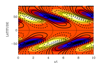
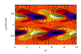
Figure 2: Butterfly diagram for a overshoot dynamo solution with no meridional circulation and two different angular dependence of the $\alpha$-effect. In the left panel the $\alpha$-effect is proportional to $\cos\theta$ and the solution has $C_{\alpha}=19.34$, $C_{\varOmega}=3000$, and $C_{\omega}=33.22$. The solid and dashed lines represent the radial field at the surface (solid for negative $B_{r}$), and blue is for negative toroidal field. The right panel represents instead a model with an $\alpha$-effect proportional to $\cos\theta\,\sin^{2}\theta$ with $C_{\alpha}=15.34$ and $C_{\omega}=23.02$. (colour online)

It is interesting to see what happens for an angular dependence of the type $\cos\theta\sin^{2}\theta$ for the $\alpha$-term since the field regeneration due to the dynamo action occurs at lower latitude in this case. The solution for a positive $\alpha$-term is depicted in the right panel of figure (2). In this case the dynamo action occurs around latitudes at which $\partial\varOmega/\partial r\approx 0$ and two distinct branches, one equatorward caused by the $\partial\varOmega/\partial r<0$ at high latitudes and the other poleward, at lower latitude, caused by $\partial\varOmega/\partial r<0$ are present. The poleward migration of the butterfly diagram at low latitude and the phase relation are clearly not consistent with the observations. In the case of a negative $\alpha$-term the only possible solution is a stationary one, as before. The conclusion of the above calculations is that it is difficult to imagine that a simple overshoot dynamo can successfully reproduce the observed features of the solar cycle, difficulties also noticed in earlier investigations (Brandenburg and Rüdiger, 1995).

The situation radically changes in the flux-dominated regime, $C_{u}\gg 1$ as one can see in figure (3) as in this case the meridional circulation transports the flux at lower latitudes. This solution is characterized by a flow $U=27\,{\rm m\,s^{-1}}$ with $\eta_{t}=4.66\;10^{11}{\rm cm^{2}s^{-1}}$ so that $C_{u}=400$.

Figure 3: The temporal evolution of the magnetic field for a solution with $C_{u}=400$, $C_{\alpha}=19.34$, $C_{\varOmega}=30000$, and frequency $C_{\omega}=102$ which imply a period of about $20$ yrs and a flow of $27\,{\rm m\,s^{-1}}$. The left part are the isocontours line of the toroidal field, with solid line for negative $B_{\phi}$ and dashed line for positive value of the field. The right part represents of the streamlines of the poloidal field given by contours of $Ar\sin\theta$. Solid line are for negative values of $A$.

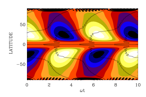
Figure 4: Butterfly diagram and phase relation for the solution presented in figure (3). (colour online)

The relevant question is to discuss the parity of the solutions as a function of the strength of the meridional circulation since a strong equatorward flow at the bottom of the convection zone can easily favor a quadrupolar parity. In fact in this case the field is by definition non-zero at the equator and the presence of the meridional circulation can help the occurrence of solutions with this symmetry. Usually only a small window in the parameter space is consistent with the observations (Bonanno et al., 2006).

However, as it is shown in figure (5) the critical $C_{\alpha}$ value is significantly smaller for dipolar solutions (solid line) than for quadrupolar solutions (dashed line), at variance with previous investigations where the difference in the critical dynamo numbers between dipolar and quadrupolar solution was not found to be very significative (Bonanno et al., 2002). It is important to stress that the evolution of the critical dynamo number $C_{\alpha}$ and the period is not a monotonic function of the meridional circulation, in general. As it is clear from figure (5) there are essentially two different scaling regimes for weak and for strong flow. In the first case the meridional circulation does not significantly affect the behavior of the dynamo wave, while at large value of the flow, the period decreases as the flow increases. The two scaling regimes are separated by a region of stationary solution around $7\,{\rm ms^{-1}}$ for an eddy diffusivity of $\eta_{t}=4.66\;10^{11}{\rm cm^{2}s^{-1}}$. This result is in agreement with the findings of previous studies (Bonanno et al., 2002, 2006) and it is not changed by the presence of a strong flow with a deep stagnation point. I conclude that the difference with the findings of Pipin and Kosovichev (2011) are mainly due to the inclusion (in that work) of the ${\bm\varOmega}\times{\bm J}$ contribution in the turbulent electromotive force (see their figure 5 where a saturation of the period seems to occur instead).

Figure 5: The critical dynamo numbers (left panel) and the period (right panel) of the solutions as a function of the meridional circulation for dipolar solutions (solid line) and quadrupolar solution (dashed lines) for an eddy diffusivity of $\eta_{t}=4.66\;10^{11}{\rm cm^{2}s^{-1}}$

4 Conclusions

The results presented in this investigation suggest that a standard $\alpha^{2}\varOmega$ mean field dynamo with a deep meridional circulation and an $\alpha$-effect located in the overshoot layer reproduces the migration of the toroidal belts at lower latitude in dynamo models with heliosesimically derived rotation law. At variance with previous studies (with the exception of the recent work by Pipin & Kosovichev 2011), the return flow is of the same order of the surface flow, and the solutions are clearly dominated by models with dipolar parity.

In this investigation the supercritical dynamo action has not been considered. This point was investigated (for a different flow pattern) in Jouve et al. (2008) where it was shown that values of $C_{\alpha}$ about ten times supercritical does not significantly change the nature of the solution, even in the flux-transport regime. On the other hand, the difference between dipolar and quadrupolar solutions in the flux-dominated regime are rather significant, and one could argue that at least for not too large supercritical dynamo numbers the conclusions of this investigations will still be valid.

The idea of determining the stagnation point of the flow by the maximum of the convective fluxes in the convection zone, as suggested by Durney (2000), leads to successful models of the meridional circulation in flux-dominated dynamo. It would be important to extend the findings of this work to the stellar case, at least for slowly rotating solar-like stars.

References

- Bonanno et al. (2002) Bonanno, A.; Elstner, D., Rüdiger, G., Belvedere, G. , “Parity properties of an advection-dominated solar -dynamo,” Astron. Astrophys. 390, 673-680 (2002).
- Bonanno et al. (2006) Bonanno, A.; Elstner, D., Belvedere, G. , “Advection-dominated solar dynamo model with two-cell meridional flow and a positive -effect in the tachocline” Astron. Nach. 327, 680- (2006).
- Brandenburg and Rüdiger (1995) Brandenburg, A. and Rüdiger, G. , “A solar dynamo in the overshoot layer: cycle period and butterfly diagram,” Astron. Astrophys. 296, 557-566 (1995).
- Bonanno and Urpin (2011) Bonanno, A.; Urpin, V., “Resonance instability of axially symmetric magnetostatic equilibria,” Phys. Rev. E 84, 056310- (2011).
- Chatterjee et al. (2004) Chatterjee, P.; Nandy, D.; Choudhuri, A. R., “Full-sphere simulations of a circulation-dominated solar dynamo: Exploring the parity issue,” Astron. Astrophys. 427, 1019-1030 (2004).
- Dikpati and Charbonneau (1999) Dikpati, M., Charbonneau, P. , “A Babcock-Leighton Flux Transport Dynamo with Solar-like Differential Rotation,” Astrophys. J. 518, 508-520 (1999).
- Dikpati and Gilman (2001) Dikpati, M. and Gilman, P.A. , “Flux-Transport Dynamos with -Effect from Global Instability of Tachocline Differential Rotation: A Solution for Magnetic Parity Selection in the Sun,” Astrophys. J. 559, 428-442 (2001).
- Durney (2000) Durney, B. R. , “Meridional Motions and the Angular Momentum Balance in the Solar Convection Zone,” Astrophys. J. 528, 486-492 (2000).
- Gellert et al. (2001) Gellert, M. and Rüdiger and Hollerbach, R. , “Helicity and -effect by current-driven instabilities of helical magnetic fields,” Monthly Notices Roy. Astron. Soc. 414, 2696-2701 (2011).
- Guerrero and de Gouveia Dal Pino (2008) Guerrero, G. and de Gouveia Dal Pino, E. M., “How does the shape and thickness of the tachocline affect the distribution of the toroidal magnetic fields in the solar dynamo?” Astron. Astrophys. 485, 267-349 (2008).
- Jouve et al. (2008) Jouve et al., “A solar mean field dynamo benchmark,” Astron. Astrophys. 483, 949-960 (2008).
- Küker et al. (2001) Küker, M., Rüdiger, G., Schultz, M. , “Circulation-dominated solar shell dynamo models with positive -effect,” Astron. Astrophys. 374, 301-308 (2001).
- Küker and Rüdiger, (2008) Küker, M., Rüdiger, G.,, “Modelling solar and stellar differential rotation,” Journal of Physics: Conference Series 118, 012029- (2008).
- Küker et al. (2011) Küker, M., Rüdiger, G., Kitchatinov, L.L., “The differential rotation of G dwarfs,” Astron. Astrophys. 530, A48- (2011).
- Parker (1955) Parker, E. N., “Hydromagnetic dynamo models,” Astrophys. J. 122, 293-314 (1955).
- Parker (1993) Parker, E. N., “A solar dynamo surface wave at the interface between convection and nonuniform rotation,” Astrophys. J. 408, 707-719 (1993).
- Pipin and Kosovichev (2011) Pipin, V.V., Kosovichev, A.G., “Mean-field Solar Dynamo Models with a Strong Meridional Flow at the Bottom of the Convection Zone,” Astrophys. J. 738, 104-112 (2011).
- Spiegel and Zahn (1992) Spiegel, E. A. and Zahn, J.-P., “The solar tachocline,” Astron. Astrophys. 265, 106-114 (1992).
- Steenbeck et al. (1966) Steenbeck, M., Krause, F., Karl-Heinz Rädler, , “Berechnung der mittleren Lorentz-Feldst rke für ein elektrisch leitendes Medium in turbulenter, durch Coriolis-Kräfte beeinflusster Bewegung,” Zeitschrift für Naturforschung 21, 369- (1966).