Mean-field closure parameters for passive scalar turbulence

Abstract

Direct numerical simulations of isotropically forced homogeneous stationary turbulence with an imposed passive scalar concentration gradient are compared with an analytical closure model which provides evolution equations for the mean passive scalar flux and variance. Triple correlations of fluctuations appearing in these equations are described in terms of relaxation terms proportional to the quadratic correlations. Three methods are used to extract the relaxation timescales $\tau_{i}$ from direct numerical simulations. Firstly, we insert the closure ansatz into our equations, assume stationarity, and solve for $\tau_{i}$. Secondly, we use only the closure ansatz itself and obtain $\tau_{i}$ from the ratio of quadratic and triple correlations. Thirdly we remove the imposed passive scalar gradient and fit an exponential decay law to the solution.

We vary the Reynolds (Re) and Péclet (Pe) numbers while keeping their ratio at unity and the degree of scale separation and find for large Re fair correspondence between the different methods. The ratio of the turbulent relaxation time of passive scalar flux to the turnover time of turbulent eddies is of the order of three, which is in remarkable agreement with earlier work. Finally we make an effort to extract the relaxation timescales relevant for the viscous and diffusive effects. We find two regimes which are valid for small and large Re, respectively, but the dependence of the parameters on scale separation suggests that they are not universal.

1 Introduction

Fluid flows in astrophysical bodies are most often highly turbulent. Direct modeling of such high-Reynolds-number flows is currently impossible. Consequently, greatly enhanced diffusivities or modified diffusion operators are often applied in simulations [6]. Such models are challenging in terms of the required computational resources, so wide-ranging parameter studies cannot be performed.

An alternative approach is to separate the large and small scales, and derive equations for the former in which correlations of small-scale quantities are parameterized. This is usually referred to as mean-field theory, see e.g. [17, 13, 21, 22]. Various schemes have been introduced to close the equations for the correlations of small-scale quantities. In astrophysics, the second-order correlation approximation (SOCA), and the minimal $\tau$ approximation (MTA, see e.g. [1, 2]) are widely used. The relevant relaxation time in MTA has been determined numerically for passive scalar transport [5] as well as for the $\alpha$ effect in mean-field electrodynamics [7, 8]. Another approach, related to the MTA, where a relaxation term is invoked to describe the higher order correlations has been introduced in [18]. In this ‘Ogilvie approach’ several nondimensional coefficients are invoked to describe physically motivated parameterizations of the higher order correlations in terms of relaxation and isotropization terms. This model has been applied to different physical setups in order to calibrate the coefficients [9, 16, 14, 10].

The validity of the various approximations can in principle be tested by comparing with direct simulations in the same parameter regime. In practise this is often not easy due to the limited parameter range accessible by the simulations. The starting point for such studies has been isotropically forced homogeneous turbulence under the influence of rotation [12] and/or shear [24]. In a recent work, the timescales related to diffusion and isotropization that appear in the Ogilvie approach have been studied [23]. In the present study we extend the work of [23] to the passive scalar case.

2 Mean-field modelling

2.1 Ideal case

Let us consider the transport of a passive scalar under the influence of a turbulent fluid motion. For simplicity we assume a homogeneous, incompressible fluid and neglect at first diffusion and viscous dissipation. Then the governing equations for the concentration of the passive scalar, $C$, and the fluid velocity $U$ read

$$\frac{\partial{C}}{\partial\hskip 0.59998pt{t}} = -\mbox{\boldmath$\nabla$}{}\cdot(\mbox{\boldmath$U$}{}C)=-\mbox{\boldmath$U$}{}\cdot\mbox{\boldmath$\nabla$}{}C,$$ (1)

$$\frac{\partial{\mbox{\boldmath$U$}{}}}{\partial\hskip 0.59998pt{t}} = -(\mbox{\boldmath$U$}{}\cdot\mbox{\boldmath$\nabla$}{})\mbox{\boldmath$U$}{}-\frac{1}{\rho}\mbox{\boldmath$\nabla$}{}P+\mbox{\boldmath$F$}{},\quad\mbox{\boldmath$\nabla$}{}\cdot\mbox{\boldmath$U$}{}=0,$$ (2)

where $P$ is the pressure, $\rho$ is the constant density and $F$ is a forcing function with $\mbox{\boldmath$\nabla$}{}\cdot\mbox{\boldmath$F$}{}=0$ (with the unit ‘force per mass’). Upon introduction of a Reynolds averaging procedure, indicated by an overbar, $C$ and $U$ are decomposed into mean and fluctuating parts, $C=\overline{C}+c$, $\mbox{\boldmath$U$}{}=\overline{\bm{U}}+\mbox{\boldmath$u$}{}$. The fluctuating fields, represented by lowercase letters, are then governed by

$$\frac{\partial{c}}{\partial\hskip 0.59998pt{t}} = -\mbox{\boldmath$u$}{}\cdot\mbox{\boldmath$\nabla$}{}\overline{C}-\overline{\bm{U}}\cdot\mbox{\boldmath$\nabla$}{}c-(\mbox{\boldmath$u$}{}\cdot\mbox{\boldmath$\nabla$}{}c)^{\prime},$$ (3)

$$\frac{\partial{\mbox{\boldmath$u$}{}}}{\partial\hskip 0.59998pt{t}} = -(\mbox{\boldmath$u$}{}\cdot\mbox{\boldmath$\nabla$}{})\overline{\bm{U}}-(\overline{\bm{U}}\cdot\mbox{\boldmath$\nabla$}{})\mbox{\boldmath$u$}{}-\left((\mbox{\boldmath$u$}{}\cdot\mbox{\boldmath$\nabla$}{}){\mbox{\boldmath$u$}{}}\right)^{\prime}-\frac{1}{\rho}\mbox{\boldmath$\nabla$}{}p+\mbox{\boldmath$f$}{},$$ (4)

where the prime indicates extraction of the fluctuating part, e.g., $(\mbox{\boldmath$u$}{}c)^{\prime}=\mbox{\boldmath$u$}{}c-\overline{\mbox{\boldmath$u$}{}c}$. Simplifying further, we stipulate the absence of a mean velocity $\overline{\bm{U}}$ and assume that the forcing has no mean part, i.e., $\mbox{\boldmath$F$}{}=\mbox{\boldmath$f$}{}$. In the present case, the goal of mean-field modeling consists in deriving a closed equation for the mean concentration $\overline{C}$. From (1) and (3), together with $\overline{\bm{U}}=\bm{0}$ we obtain directly

$$\frac{\partial{\overline{C}}}{\partial\hskip 0.59998pt{t}}=-\mbox{\boldmath$\nabla$}{}\cdot\overline{\mbox{\boldmath${\cal F}$}}{}$$ (5)

with the mean density of the passive scalar flux, $\overline{\mbox{\boldmath${\cal F}$}}{}=\overline{c\mbox{\boldmath$u$}{}}$. So the task of closing (5) reduces to representing $\overline{\mbox{\boldmath${\cal F}$}}{}$ by the mean concentration $\overline{C}$. In the standard mean-field approach, (3) is solved for a prescribed fluctuating velocity $u$, usually under some simplifying assumptions which inevitably limit the applicability of the obtained results. The solution is employed to express $\overline{\mbox{\boldmath${\cal F}$}}{}$ in terms of $\overline{C}$. Alternatively, one can abstain from deriving such an explicit solution for the fluctuating concentration $c$ and instead strive for establishing an evolution equation for $\overline{\mbox{\boldmath${\cal F}$}}{}$ which of course again has to be closed in the sense that the only variables occurring are the mean quantities $\overline{C}$ and $\overline{\mbox{\boldmath${\cal F}$}}{}$ themselves. Such an equation is obtained by multiplying (3) with $u$ and (4) with $c$, summing up and averaging, arriving at

$$\frac{\partial{\overline{\mbox{\boldmath${\cal F}$}}{}}}{\partial\hskip 0.59998pt{t}}=-\overline{\mbox{\boldmath$u$}{}\mbox{\boldmath$\nabla$}{}\cdot(\mbox{\boldmath$u$}{}\overline{C})}-\overline{\mbox{\boldmath$u$}{}\mbox{\boldmath$\nabla$}{}\cdot(\mbox{\boldmath$u$}{}c)}-\overline{c\left((\mbox{\boldmath$u$}{}\cdot\mbox{\boldmath$\nabla$}{})\mbox{\boldmath$u$}{}\right)}-\frac{1}{\rho}\,\overline{c\mbox{\boldmath$\nabla$}{}p}+\overline{c\mbox{\boldmath$f$}{}}.$$ (6)

By virtue of the incompressibility of the fluid the fluctuating pressure $p$ can be expressed by the velocity fluctuations:

$$\mbox{\boldmath$\nabla$}{}^{2}p=-\rho\left(\frac{\partial{u_{i}}}{\partial\hskip 0.59998pt{x_{j}}}\frac{\partial{u_{j}}}{\partial\hskip 0.59998pt{x_{i}}}\right)^{\prime}$$ (7)

which for an infinitely extended medium and vanishing $p$ at infinity is readily solved by

$$p=\frac{\rho}{4\pi}\int\frac{\left({\partial{u_{i}}/\partial{x_{j}}}{\partial{u_{j}}/\partial{x_{i}}}\right)^{\prime}(\bm{x}^{\prime})}{|\bm{x}-\bm{x}^{\prime}|}d\,^{3}x^{\prime}.$$ (8)

Now we can conclude that the second, third, and fourth terms on the r.h.s. of (6) are quadratic in $u$ and linear in $c$, hence represent third order correlations. Following [10] we introduce here the closure assumption

$$-\overline{\mbox{\boldmath$u$}{}\mbox{\boldmath$\nabla$}{}\cdot(\mbox{\boldmath$u$}{}c)}-\overline{c\left((\mbox{\boldmath$u$}{}\cdot\mbox{\boldmath$\nabla$}{})\mbox{\boldmath$u$}{}\right)}-\frac{1}{\rho}\,\overline{c\mbox{\boldmath$\nabla$}{}p}=-\frac{\overline{\mbox{\boldmath${\cal F}$}}{}}{\tau_{6}}$$ (9)

with a relaxation time $\tau_{6}$. Upon further neglect of the correlation $\overline{c\mbox{\boldmath$f$}{}}$, we arrive at

$$\frac{\partial{\overline{\cal F}_{i}}}{\partial\hskip 0.59998pt{t}}=-\overline{u_{i}u_{j}}\,\frac{\partial{\overline{C}}}{\partial\hskip 0.59998pt{x_{j}}}-\frac{\overline{\cal F}_{i}}{\tau_{6}}=-\overline{\cal R}_{ij}\frac{\partial{\overline{C}}}{\partial\hskip 0.59998pt{x_{j}}}-\frac{\overline{\cal F}_{i}}{\tau_{6}},$$ (10)

which governs the evolution of $\overline{\mbox{\boldmath${\cal F}$}}{}$. Here, $\overline{\cal R}_{ij}=\overline{u_{i}u_{j}}$ stands for the Reynolds stress tensor. Since a passive scalar would not act back onto the velocity, $\overline{\cal R}_{ij}$ can here be considered given and the closure is completed. Nevertheless, in the presence of rotation, shear, or gravity, (4) contributes quadratic correlations to (6) even in the kinematic case; see, e.g., [12, 24, 15]. Equation (10) is similar to the penultimate row of Eq. (53) in [10] when replacing temperature perturbation $\Theta$ by $C$ and neglecting the buoyancy term. Note that for small $\tau_{6}$, that is, fast relaxation, $\overline{\cal F}_{i}$ will follow the inhomogeneity in (10) almost instantaneously, hence

$$\overline{\cal F}_{i}\approx-\tau_{6}\overline{\cal R}_{ij}\,\frac{\partial{\overline{C}}}{\partial\hskip 0.59998pt{x_{j}}},$$ (11)

and we may interpret $\tau_{6}\overline{\cal R}_{ij}$ as a turbulent diffusivity tensor. For a discussion of its relationship to traditional mean-field results, see Sect. 2.5.

To facilitate further comparisons to [10, 4], where an additional evolution equation for the mean temperature perturbation variance $\overline{\Theta^{2}}$ is derived, we give here an analogous equation for $\overline{c^{2}}=\overline{\cal Q}$, although it is not necessary for completing the closure:

$$\frac{\partial{\overline{\cal Q}}}{\partial\hskip 0.59998pt{t}}=-2\overline{c\mbox{\boldmath$u$}{}}\cdot\mbox{\boldmath$\nabla$}{}\overline{C}-2\overline{c(\mbox{\boldmath$u$}{}\cdot\mbox{\boldmath$\nabla$}{}c)}.$$ (12)

We note in passing that the $\overline{\cal Q}$ term becomes important in reacting flows [4]. Setting

$$-2\overline{c(\mbox{\boldmath$u$}{}\cdot\mbox{\boldmath$\nabla$}{}c)}=-\overline{\cal Q}/\tau_{7}$$ (13)

with another relaxation time $\tau_{7}$, the closed equation reads

$$\frac{\partial{\overline{\cal Q}}}{\partial\hskip 0.59998pt{t}}=-2\overline{\mbox{\boldmath${\cal F}$}}{}\cdot\mbox{\boldmath$\nabla$}{}\overline{C}-\frac{\overline{\cal Q}}{\tau_{7}}$$ (14)

and we have full analogy to the last row of Eq. (53) in [10].

Until now we have not constrained the properties of the turbulence, in particular we have not required isotropy or homogeneity. For example, inhomogeneous turbulence could be thought of giving rise to position-dependent relaxation times. However, from a strict point of view, the $\tau$ ansatz (9) is only consistent with an isotropic or uni-axial $u$ turbulence where the preferred direction of the latter coincides with the direction of $\overline{\mbox{\boldmath${\cal F}$}}{}$. Consequently, turbulent properties of $u$ must not change along any other direction. The same restrictions should of course hold for the concentration fluctuations $c$, but this is in conflict with the presence of the second preferred direction $\mbox{\boldmath$\nabla$}{}\overline{C}$ in this turbulence. Hence, (9) can be strictly justified only under very specific circumstances.

For that reason and for the sake of simplicity, we specify now the mean as horizontal average, i.e., as average over all $x$ and $y$. Consequently, all mean quantities depend on $z$ only and only the $z$ component of $\overline{\mbox{\boldmath${\cal F}$}}{}$ is relevant. If we further restrict $u$ to have at best a $z$ anisotropy, then there is only a single preferred direction, namely that of $\overline{\mbox{\boldmath${\cal F}$}}{}$ and the ansatz (9) is legitimate. The system of mean field equations then simplifies to

$$\frac{\partial{\overline{C}}}{\partial\hskip 0.59998pt{t}}=-\frac{\partial{\overline{\cal F}_{z}}}{\partial\hskip 0.59998pt{z}},\quad\frac{\partial{\overline{\cal F}_{z}}}{\partial\hskip 0.59998pt{t}}=-\overline{\cal R}_{zz}\frac{\partial{\overline{C}}}{\partial\hskip 0.59998pt{z}}-\frac{\overline{\cal F}_{z}}{\tau_{6}},\quad\frac{\partial{\overline{\cal Q}}}{\partial\hskip 0.59998pt{t}}=-2\overline{\cal F}_{z}\frac{\partial{\overline{C}}}{\partial\hskip 0.59998pt{z}}-\frac{\overline{\cal Q}}{\tau_{7}}\,.$$ (15)

where $\overline{\cal R}_{zz}$, $\tau_{6}$ and $\tau_{7}$ could still depend on $z$ and $t$. Assuming now further homogeneous and statistically stationary fluctuations $u$ and $c$ and a uniform gradient of $\overline{C}$, $\mbox{\boldmath$\nabla$}{}\overline{C}=(0,0,G)$, a stationary regime of (15) should be given by

$$\overline{\cal F}_{z}=\mbox{const.}=-\tau_{6}\overline{\cal R}_{zz}G,\quad\overline{\cal Q}=-2\tau_{7}\overline{\cal F}_{z}G=2\tau_{6}\tau_{7}\overline{\cal R}_{zz}G^{2}.$$ (16)

Let us now assume that in a direct numerical simulation (DNS) Eqs. (1) and (2) with an appropriately defined forcing $f$ and an imposed uniform $G$ are integrated in time until a statistically stationary regime is established. Extracting now all mean quantities occurring in (16) from the numerical solution and assuming validity of the model (10) and (14), it is obviously possible to determine the crucial relaxation times $\tau_{6,7}$ from such runs (method M1). On the other hand, $\tau_{6,7}$ should of course also obey their defining relations (9) and (13). The third-order correlations $\overline{\mbox{\boldmath$u$}{}\mbox{\boldmath$\nabla$}{}\cdot(\mbox{\boldmath$u$}{}c)}$, $\overline{c\left((\mbox{\boldmath$u$}{}\cdot\mbox{\boldmath$\nabla$}{})\mbox{\boldmath$u$}{}\right)}$, $\overline{c\mbox{\boldmath$\nabla$}{}p}$ and $\overline{c(\mbox{\boldmath$u$}{}\cdot\mbox{\boldmath$\nabla$}{}c)}$ are again accessible in the DNS results and open up an independent path for determining the relaxation times (method M2). At the same time, it can also be checked to what extent the neglect of $\overline{c\mbox{\boldmath$f$}{}}$ is justified.

Another approach to extract $\tau_{6,7}$ is available from decay experiments, for which, after having reached a stationary state in the DNS, the imposed gradient of $\overline{C}$ is switched off. Then, according to (10) and (14), $\overline{\mbox{\boldmath${\cal F}$}}{}$ and $\overline{\cal Q}$ should decay uniformly in space and exponentially in time with the increment $\tau_{6}^{-1}$ and $\tau_{7}^{-1}$, respectively, and can be identified with the decay rates measured in the DNS (method M3). An exemplification of this method is shown in Figure 1.

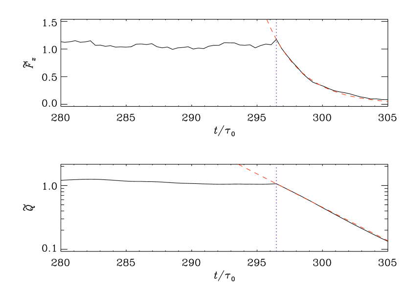
Figure 1: Method M3 of estimating the timescales $\tau_{6,7}$ from decaying $\overline{\cal F}_{z}$ and $\overline{\cal Q}$ normalized by their mean values in the stationary state: $\widetilde{\overline{\cal Q}}=\langle\overline{\cal Q}\rangle_{z}/\langle\overline{\cal Q}\rangle_{zt}$, $\widetilde{\overline{\cal F}}_{z}=\langle\overline{\cal F}_{z}\rangle_{z}/\langle\overline{\cal F}\rangle_{zt}$, where $\langle\rangle_{\xi}$ denotes averaging over the variable $\xi$. Dotted vertical line: switching off of the imposed mean concentration gradient $G$. $\tau_{0}=(u_{\rm rms}k_{\rm f})^{-1}$ – dynamical time. Dashed red lines: fit by exponentials in $t/\tau_{0}$.

The goal of this paper consists in systematically testing the validity of the presented closure assumptions for a range of Reynolds and Péclet numbers as well as different levels of scale separation. From this we expect hints with respect to the validity of the Garaud model of turbulent convection [10].

2.2 Non-ideal effects

Admitting now diffusion and viscous dissipation, we have to add the term $\kappa\mbox{\boldmath$\nabla$}{}^{2}C$ with the diffusivity $\kappa$ on the r.h.s. of (1) and $\nu\mbox{\boldmath$\nabla$}{}^{2}\mbox{\boldmath$U$}{}$ with the kinematic viscosity $\nu$ on the r.h.s. of (2). Consequently, in the evolution equation (6) for $\overline{\mbox{\boldmath${\cal F}$}}{}$, the additional terms $\nu\overline{c\mbox{\boldmath$\nabla$}{}^{2}\mbox{\boldmath$u$}{}}$ and $\kappa\overline{\mbox{\boldmath$u$}{}\mbox{\boldmath$\nabla$}{}^{2}c}$ occur on the r.h.s.. Rewriting their sum as

$$\nu\mbox{\boldmath$\nabla$}{}^{2}\overline{\cal F}_{i}-2\nu\overline{\frac{\partial{c}}{\partial\hskip 0.59998pt{x_{j}}}\frac{\partial{u_{i}}}{\partial\hskip 0.59998pt{x_{j}}}}+(\kappa-\nu)\overline{u_{i}\mbox{\boldmath$\nabla$}{}^{2}c}$$ (17)

or more symmetric, as done in [10], as

$$\frac{\nu+\kappa}{2}\mbox{\boldmath$\nabla$}{}^{2}\overline{\cal F}_{i}-(\nu+\kappa)\overline{\frac{\partial{c}}{\partial\hskip 0.59998pt{x_{j}}}\frac{\partial{u_{i}}}{\partial\hskip 0.59998pt{x_{j}}}}+\frac{\nu-\kappa}{2}\overline{\frac{\partial{}}{\partial\hskip 0.59998pt{x_{j}}}\left(c\frac{\partial{u_{i}}}{\partial\hskip 0.59998pt{x_{j}}}-u_{i}\frac{\partial{c}}{\partial\hskip 0.59998pt{x_{j}}}\right)}$$ (18)

does nevertheless not allow a representation entirely by the mean flux. Even in the (very particular) case $\kappa=\nu$ the second terms of (17) and (18) remain. As a skyhook, the second and third terms are replaced by the $\tau$-ansatz-like expression, $-\overline{\mbox{\boldmath${\cal F}$}}{}/\tau_{\nu\kappa}$ although they contain second order rather than third order correlations. Analogously, on the r.h.s. of (12), diffusion requires a term

$$2\kappa\overline{c\mbox{\boldmath$\nabla$}{}^{2}c}=\kappa\mbox{\boldmath$\nabla$}{}^{2}\overline{Q}-2\kappa\overline{(\mbox{\boldmath$\nabla$}{}c)^{2}}$$ (19)

and the second term is replaced by $-\overline{Q}/\tau_{\kappa\kappa}$. Note that diffusion of $\overline{\mbox{\boldmath${\cal F}$}}{}$ and $\overline{\cal Q}$ modelled in this way is obviously determined by the molecular (or microscopic) diffusivities.

In astrophysical applications the deviation from ideal conditions is usually small, and quantities expressing this smallness are given by the Reynolds and Péclet numbers, Re and Pe, which reflect the strength of advection relative to diffusion:

$$\mbox{\rm Re}=u_{\rm rms}\ell/\nu,\quad\mbox{\rm Pe}=u_{\rm rms}\ell/\kappa,$$ (20)

where $\ell$ is a characteristic scale of the turbulence. We will further make use of the Schmidt number $\mbox{\rm Sc}=\nu/\kappa=\mbox{\rm Pe}/\mbox{\rm Re}$.

2.3 Summary of method M2

So, summarizing all the terms used to determine $\tau_{6\nu\kappa}$ and $\tau_{7\kappa\kappa}$ from Method M2 (ideal and non-ideal, see equations (9), (13), (18) and (19)), we have

$$\frac{\overline{\cal F}_{z}}{\tau_{6\nu\kappa}}=\overline{u_{z}\mbox{\boldmath$\nabla$}{}\cdot(\mbox{\boldmath$u$}{}c)}+\overline{c\left((\mbox{\boldmath$u$}{}\cdot\mbox{\boldmath$\nabla$}{})u_{z}\right)}+\frac{1}{\rho}\,\overline{c\,\mbox{\boldmath$\nabla$}{}_{\!z}\,p}+$$

$$+(\nu+\kappa)\overline{\mbox{\boldmath$\nabla$}{}c\cdot\mbox{\boldmath$\nabla$}{}u_{z}}-\,\frac{\nu-\kappa}{2}\,\overline{\left(c\mbox{\boldmath$\nabla$}{}^{2}{u_{z}}-u_{z}\mbox{\boldmath$\nabla$}{}^{2}c\right)},$$ (21)

$$\frac{\overline{\cal Q}}{\tau_{7\kappa\kappa}}=2\left(\overline{c(\mbox{\boldmath$u$}{}\cdot\mbox{\boldmath$\nabla$}{}c)}+\kappa\overline{(\mbox{\boldmath$\nabla$}{}c)^{2}}\right).$$ (22)

2.4 Scaling of the relaxation times

For the relaxation times $\tau_{6,7,\nu\kappa,\kappa\kappa}$ some reasonable scaling assumptions are in order and we follow essentially the choices of [10]: $\tau_{6,7}$, belonging to third-order correlation terms, are expressed as $(C_{6,7}u_{\rm rms}k_{1})^{-1}$, and $\tau_{\nu\kappa,\kappa\kappa}$, belonging to diffusive second-order correlation terms are written as

$$(C_{\nu\kappa}(\nu+\kappa)k_{1}^{2}/2)^{-1}\quad\mbox{and}\quad(C_{\kappa\kappa}\kappa k_{1}^{2})^{-1},$$ (23)

respectively. The first of these expressions seems to be appropriate only for $|\nu-\kappa|\ll\nu+\kappa$, hence in general the scaling ansatz should read instead

$$\Big{(}\big{(}C_{\nu+\kappa}\frac{\nu+\kappa}{2}+C_{\nu-\kappa}(\nu-\kappa)\big{)}k_{1}^{2}\Big{)}^{-1}\!\!\!.$$ (24)

Here $k_{1}=2\pi/L$ is the smallest wavenumber consistent with the box size, $L$. The crucial question is now: are the constants $C_{6,7,\nu\kappa,\kappa\kappa}$ universal, at least for a given type of turbulence, and in particular, are they independent of the dimensionless numbers of the problem, i.e., Re and Pe, and of the degree of scale separation? A preliminary answer to this question was given in [5], where the timescales were found to show a slightly increasing trend with increasing scale separation (see their Fig. 4).

Methods M1 and M3 for determining the relaxation times described in Sect. 2.1 have now to be modified in the following way: In (16) we have to replace $\tau_{6}$ by $\tau_{6}\tau_{\nu\kappa}/(\tau_{6}+\tau_{\nu\kappa})\equiv\tau_{6\nu\kappa}$ and $\tau_{7}$ by $\tau_{7}\tau_{\kappa\kappa}/(\tau_{7}+\tau_{\kappa\kappa})\equiv\tau_{7\kappa\kappa}$. Both methods then deliver only these aggregates and we have to employ the different scalings of the relaxation times to figure out the individual constants $C_{\ast}$. In contrast, method M2 has merely to be extended to include also the additional second-order correlations showing up in (18) and (19), that is, to use expressions (21) and (22).

2.5 Comparison with traditional results

A standard mean-field approach to (1), employing SOCA, that is, neglecting $(\mbox{\boldmath$u$}{}\cdot\mbox{\boldmath$\nabla$}{}c)^{\prime}$ in (3) yields straightforwardly

$$\overline{\cal F}_{i}(t)=-\int_{0}^{\infty}\overline{u_{i}(t)u_{j}(t-\tau)}\,\frac{\partial{\overline{C}}}{\partial\hskip 0.59998pt{x_{j}}}(t-\tau)\,d\tau$$ (25)

from which, under the assumption of good temporal scale separation,

$$\overline{\cal F}_{i}(t)=-\int_{0}^{\infty}\overline{u_{i}(t)u_{j}(t-\tau)}\,d\tau\,\frac{\partial{\overline{C}}}{\partial\hskip 0.59998pt{x_{j}}}(t)=-\kappa_{ij}\frac{\partial{\overline{C}}}{\partial\hskip 0.59998pt{x_{j}}}$$ (26)

can be concluded. $\kappa_{ij}=\int_{0}^{\infty}\overline{u_{i}(t)u_{j}(t-\tau)}\,d\tau=\tau_{\rm c}\overline{u_{i}(t)u_{j}(t)}$ can readily be identified as turbulent diffusivity tensor. Here the correlation time $\tau_{c}$ is just defined by the last identity. This clearly resembles the result (10) with $\tau_{6}$ being identified with the correlation time $\tau_{c}$, the more so as for the validity of both (26) and (10) the relevant time parameter has, in a sense, to be small.

Relaxing the assumption of good temporal scale separation, that is retaining (25), we observe the presence of the so-called memory effect [11], that is, the influence of ${\partial{\overline{C}}/\partial{x_{j}}}$ at earlier times $t-\tau$ on the mean flux at time $t$ by virtue of a convolution. Performing a Fourier transform with respect to time, this convolution turns into a simple multiplication and we can write

$$\,\hat{\!\hskip 0.42677pt\overline{\cal F}}_{i}(\omega)=-\,\hat{\!\hskip 0.42677pt\kappa}_{ij}(\omega)\,\hat{\!\hskip 0.42677ptG}(\omega)$$ (27)

with a frequency-dependent turbulent diffusivity tensor $\,\hat{\!\hskip 0.42677pt\kappa}_{ij}$. This quantity is directly accessible to the test-field method as described, e.g., in [11]. Based on numerical simulations, and without resorting to SOCA, it has been found that for homogeneous isotropic turbulence a satisfactory approximation is accomplished already by

$$\hat{\kappa}_{ij}(\omega)=\delta_{ij}\frac{\kappa_{0}}{1-{\rm i}\omega\tau_{\kappa}}$$ (28)

where $\kappa_{0}$ is the turbulent diffusivity for stationary fields and $\tau_{\kappa}$ is independent of $\omega$. A slightly better fit is provided by

$$\hat{\kappa}_{ij}(\omega)=\delta_{ij}(1+K)\kappa_{0}\frac{1-{\rm i}\omega\tau_{\kappa}}{(1-{\rm i}\omega\tau_{\kappa})^{2}+K}$$ (29)

with a constant $K$. Turning back to the physical space the first approximation (28) is equivalent to

$$\overline{\mbox{\boldmath${\cal F}$}}{}+\tau_{\kappa}\frac{\partial{\overline{\mbox{\boldmath${\cal F}$}}{}}}{\partial\hskip 0.59998pt{t}}=-\kappa_{0}\mbox{\boldmath$\nabla$}{}\overline{C}$$ (30)

or

$$\frac{\partial{\overline{\mbox{\boldmath${\cal F}$}}{}}}{\partial\hskip 0.59998pt{t}}=-\frac{\kappa_{0}}{\tau_{\kappa}}\mbox{\boldmath$\nabla$}{}\overline{C}-\frac{\overline{\mbox{\boldmath${\cal F}$}}{}}{\tau_{\kappa}}.$$ (31)

Again, there is striking similarity to (10). Thus by comparing $\tau_{6}$ to numerical results for $\tau_{\kappa}$, a further independent way of checking (9) is provided. The second fit (29) gives [11]

$$(1+K)\overline{\mbox{\boldmath${\cal F}$}}{}+2\tau_{\kappa}\frac{\partial{\overline{\mbox{\boldmath${\cal F}$}}{}}}{\partial\hskip 0.59998pt{t}}+\tau_{\kappa}^{2}\frac{\partial{\,{}^{2}\overline{\mbox{\boldmath${\cal F}$}}{}}}{\partial\hskip 0.59998pt{t^{2}}}=-(1+K)\kappa_{0}\mbox{\boldmath$\nabla$}{}\left(\overline{C}+\tau_{\kappa}\frac{\partial{\overline{C}}}{\partial\hskip 0.59998pt{t}}\right)$$ (32)

indicating the potential importance of higher temporal and mixed temporal/spatial derivatives. Note that (31) and (32) are only valid for perfect scale separation in space.

For the general case of imperfect scale separation both with respect to space and time, we refer here to [20], albeit this work deals with the mean electromotive force of MHD rather than with the mean flux of passive scalar transport. In that work, non-locality due to imperfect spatial scale separation shows up in the form of a diffusion term $\eta_{\scriptscriptstyle\cal E}\mbox{\boldmath$\nabla$}{}^{2}\overline{\mbox{\boldmath${\cal E}$}}{}$ in the evolution equation for $\overline{\mbox{\boldmath${\cal E}$}}{}$ with a diffusivity $\eta_{\scriptscriptstyle\cal E}$ occasionally even larger than, but of the order of the SOCA estimate of the turbulent diffusivity in the high-conductivity limit, $\eta_{\rm t}=\tau_{\rm c}u_{\rm rms}^{2}/3$. Clearly, this value can be very different from the molecular diffusivity. When comparing with the diffusion term for $\overline{\mbox{\boldmath${\cal F}$}}{}$ identified in (17) or (18) where only the microscopic diffusivities occur we have to state that the Ogilvie approach deviates in this respect significantly from what we expect from the traditional approach. To reconcile them, possible diffusion terms $\sim\mbox{\boldmath$\nabla$}{}^{2}\overline{\mbox{\boldmath${\cal F}$}}{}$ and $\sim\mbox{\boldmath$\nabla$}{}^{2}\overline{\cal Q}$ had to be taken into account in the parameterizing ansatzes.

2.6 Significance of method comparisons

Let us finally discuss what is really “tested” by comparisons of the results of the different methods M1–M3. For an incompressible fluid with the specific conditions of our model and under the assumption that no higher than the first order temporal derivative occurs, an ansatz for $\overline{\mbox{\boldmath${\cal F}$}}{}$ analogous to (16),

$$\frac{\partial{\overline{\cal F}_{z}}}{\partial\hskip 0.59998pt{t}}=-K_{1}G-K_{2}\overline{\cal F}_{z},$$ (33)

is exhaustive, as

1. $c$ and hence $\overline{\mbox{\boldmath${\cal F}$}}{}$ is quite generally a linear and homogeneous functional of $\mbox{\boldmath$\nabla$}{}\overline{C}$ (even when the correlation $\overline{c\mbox{\boldmath$f$}{}}$ is not neglected), and

2. $G$ and hence $\overline{\cal F}_{z}$ are spatially constant, both in the statistically steady state and during the decay of $\overline{\cal F}_{z}$. (That is why the diffusive term $\propto\mbox{\boldmath$\nabla$}{}^{2}\overline{\cal F}_{z}$ is absent.)

Note, however, that $K_{1}=\overline{\cal R}_{zz}$ as in (16) is an assumption because a contribution proportional to $\mbox{\boldmath$\nabla$}{}C$ or ${\partial{\overline{\cal F}_{z}}/\partial{t}}$ can also be provided by the triple correlations, the diffusive terms or by $\overline{c\mbox{\boldmath$f$}{}}$.

Since the passive scalar $C$ does not influence the turbulent velocity, the coefficients $K_{1,2}$ are completely determined by $u$ and hence true constants. Consequently, any comparison of the methods M1, M2, and M3 tests the influence of

1. the weak compressibility of the fluid in our simulations, and

2. deviations of the simulated velocity turbulence from homogeneity, isotropy and statistical stationarity.

Note, that the first influence can in principle be made arbitrarily small by increasing the sound speed $c_{\rm s}$ in the numerical model, likewise the second by increasing scale separation and extending time ranges for averaging.

A comparison of M1 and M3 tests in addition the justification of

1. the neglect of higher temporal derivatives of $\overline{\cal F}_{z}$,

2. the assumption $K_{1}=\overline{\cal R}_{zz}$ which was employed in calculating $\tau_{6\nu\kappa}=1/K_{2}$ from the steady state.

On the other hand, a comparison of M1 and M2 tests again the assumption $K_{1}=\overline{\cal R}_{zz}$ and specifically to what extent the neglect of the correlation $\overline{c\mbox{\boldmath$f$}{}}$ is legitimate. This affects $\tau_{6\nu\kappa}$ only, so we expect that here the discrepancies between M1 and M2 are more pronounced than in $\tau_{7\kappa\kappa}$.

With respect to the evolution equation for $\overline{\cal Q}$ in (15), the same conclusions hold true as far as only the steady state and the free decay with $G=0$ are taken into account. However, considering a general transient as a consequence of switching $G$ between two non-zero constants, a richer behavior should appear which perhaps allows further reaching conclusions.

3 Numerical setup

In order to take benefit of the capabilities of the Pencil Code  we solve instead of the incompressible system (1) and (2) the corresponding equations for a compressible, but isothermal fluid

$$\frac{\partial{\,\mbox{\boldmath$U$}{}}}{\partial\hskip 0.59998pt{t}} = -\mbox{\boldmath$U$}{}\cdot\mbox{\boldmath$\nabla$}{}\mbox{\boldmath$U$}{}-\mbox{\boldmath$\nabla$}{}H+{\mbox{\boldmath$f$}{}}+2\nu\left(\mbox{\boldmath$\nabla$}{}\cdot\mbox{\boldmath$S$}{}(\mbox{\boldmath$U$}{})+\mbox{\boldmath$S$}{}(\mbox{\boldmath$U$}{})\cdot\mbox{\boldmath$\nabla$}{}H/c_{\rm s}^{2}\right)$$ (34)

$$\frac{\partial{H}}{\partial\hskip 0.59998pt{t}} = -\mbox{\boldmath$U$}{}\cdot\mbox{\boldmath$\nabla$}{}H-c_{\rm s}^{2}\mbox{\boldmath$\nabla$}{}\cdot\mbox{\boldmath$U$}{},$$ (35)

$$\frac{\partial{\,C}}{\partial\hskip 0.59998pt{t}} = -\mbox{\boldmath$\nabla$}{}\cdot(C\mbox{\boldmath$U$}{})+\kappa\mbox{\boldmath$\nabla$}{}^{2}C,$$ (36)

where we employ the pseudo enthalpy $H=c_{\rm s}^{2}\ln\rho$ instead of the density; $c_{\rm s}$ is the constant speed of sound and $\mbox{\boldmath$S$}{}(\mbox{\boldmath$U$}{})$ the trace-less rate-of-strain tensor $S_{ij}=({\partial{U_{i}}/\partial{x_{j}}}+{\partial{U_{j}}/\partial{x_{i}}})/2-\delta_{ij}\mbox{\boldmath$\nabla$}{}\cdot\mbox{\boldmath$U$}{}/3$. Interpretation of the results of such simulations in terms of the incompressible model of course requires to keep the Mach number $u_{\rm rms}/c_{\rm s}$ small, typically $<0.1$. Then it is particularly justified to replace the correlation $\overline{c\mbox{\boldmath$\nabla$}{}p}/\rho$, included in the $\tau$ ansatz, by $\overline{c\mbox{\boldmath$\nabla$}{}h}$.

The equations are solved by equidistant sixth order finite differences in space and an explicit third order time stepping scheme with step size control for stability. The computational domain is a cube with dimension $(2\pi)^{3}$ and grid resolutions ranging from $32^{3}$ to $256^{3}$ according to the requirements raised by the values of the Reynolds and Péclet numbers and the forcing wavenumber. Boundary conditions are periodic throughout. The fluctuating force $f$ is specified such that it generates an approximately homogeneous, isotropic and statistically stationary fluctuating velocity $u$. During any integration timestep, $f$ is a frozen-in linearly polarized (i.e., non-helical) plane wave with a wave-vector which is consistent with the periodic boundary conditions and whose modulus is close to a chosen average value $k_{\rm f}$. The wave amplitude is kept fixed whereas the wavevector is randomly changing between time steps and hence $f$ is approximately $\delta$-correlated in time. For further details, see [3].

4 Results

Table 1: Results from methods M1, M2, and M3 for different values of $s=k_{\rm f}/k_{1}$. $\nu=\kappa$, $\mbox{\rm Sc}=1$.

$s$	$\rm Re$	M1		M2		M3
		$\tau_{6\nu\kappa}$	$\tau_{7\kappa\kappa}$	$\tau_{6\nu\kappa}$	$\tau_{7\kappa\kappa}$	$\tau_{6\nu\kappa}$	$\tau_{7\kappa\kappa}$
1.5	51.02-552.47	2.09-2.42	4.14-4.28	2.36-2.71	4.10-6.86	1.85-2.96	3.64-5.21
3	23.44-694.63	2.12-2.64	4.29-5.03	2.15-2.70	4.29-14.21	1.94-2.81	3.94-4.96
5	12.62-415.00	2.29-2.77	4.54-5.89	2.31-2.79	4.54-41.27	2.43-2.77	4.93-5.67
8	6.87-256.50	2.40-2.86	5.59-9.13	2.41-2.88	-21.54-34.81	2.25-2.85	5.26-7.70
10	5.06-204.34	2.09-2.87	6.00-8.06	2.10-2.93	-10.43-8.93	2.24-2.99	3.44-4.50

In general, the parameter space is spanned by the dimensionless numbers $s=k_{\rm f}/k_{1}$ (degree of scale separation), Re and Pe, in whose definitions (20) we specify the characteristic length $\ell$ for simplicity by $1/k_{\rm f}$. In the following, we will however restrict ourselves to $\mbox{\rm Re}=\mbox{\rm Pe}$, that is, $\mbox{\rm Sc}=1$ and leave the more general cases to future work. By this, we avoid in particular the complication with the scaling ansatz (23) which occurs for $\nu\neq\kappa$. For methods M1 and M2, all averaged quantities were derived from the simulations by performing in addition to the $xy$ averaging and a temporal averaging over an interval in which in particular the correlation $\overline{c^{2}}$ was found to be statistically stationary. Statistical errors were estimated by dividing this interval into three equally long parts and calculating averages over each of them. These individual averages were compared to the average over the whole interval, and the largest deviation was taken for the error estimate.

We performed a number of simulations, and extracted $\tau_{6\nu\kappa}$ and $\tau_{7\kappa\kappa}$ using methods M1, M2 and M3. The results are summarized in Table 1, where the several simulations are grouped together into different sets by the values used for the scale separation $s$. Within each set the Reynolds numbers were varied by changing $\nu$ ($=\kappa$). The timescales $\tau_{6\nu\kappa}$ and $\tau_{7\kappa\kappa}$ listed in Table 1 are also illustrated in Figures 2 and 3, respectively. We see that all three methods give quite similar results, with

$$\tau_{6\nu\kappa}/\tau_{0}\approx 2\ldots 3,\hskip 14.22636pt\mbox{and}\hskip 14.22636pt\tau_{7\kappa\kappa}/\tau_{0}\approx 7\ldots 10.$$ (37)

There are some exceptions, however. When $s=1.5$, methods M2 and M3 yield $2\lesssim\tau_{7\kappa\kappa}/\tau_{0}\lesssim 3$, unlike method M1 which stays in range given above. Moreover, although method M2 always yields positive values for $\tau_{6\nu\kappa}$, those for $\tau_{7\kappa\kappa}$ are sometimes negative. The absolute values of the M2 results can also be very high. This is because the sum of the correlations used to calculate $\tau_{7\kappa\kappa}$ may become very small. This problem manifests itself mainly in the high Reynolds number runs.

4.1 Universality of the closure ansatz

As explained in Sect. 2.2, methods M1 and M3 yield only the quantities $\tau_{6\nu\kappa}$ and $\tau_{7\kappa\kappa}$. from which the constants $C_{6,7,\nu\kappa,\kappa\kappa}$ can be extracted as follows: Recalling the scalings (23) we have:

$$\frac{1}{\tau_{6\nu\kappa}}=C_{6}u_{\rm rms}k_{1}+C_{\nu\kappa}(\nu+\kappa)\frac{k_{1}^{2}}{2},\qquad\frac{1}{\tau_{7\kappa\kappa}}=C_{7}u_{\rm rms}k_{1}+C_{\kappa\kappa}\kappa k_{1}^{2}.$$ (38)

Multiplying by the viscous time $\tau_{\rm visc}=(\nu k_{1}^{2})^{-1}$ yields

$$\frac{1}{\tilde{\tau}_{6\nu\kappa}}=C_{6}s\mbox{\rm Re}+C_{\nu\kappa},\qquad\frac{1}{\tilde{\tau}_{7\kappa\kappa}}=C_{7}s\mbox{\rm Pe}+C_{\kappa\kappa},$$ (39)

where a tilde indicates normalization by $\tau_{\rm visc}$. Hence, when considering $1/\tilde{\tau}_{6\nu\kappa}$ and $1/\tilde{\tau}_{7\kappa\kappa}$ as functions of Re (or Pe), the wanted parameters should be obtainable by a linear regression analysis. Figure 4 shows both functions (39) for different values of $s$. Obviously, a linear relation is clearly present both for large and small values of Re, but with very different fit parameters for the two ranges.

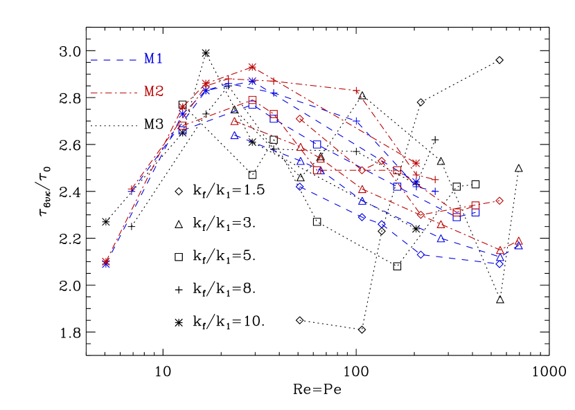
Figure 2: Comparison of relaxation timescales $\tau_{6\nu\kappa}$, normalized by the dynamical time $\tau_{0}=(u_{\rm rms}k_{f})^{-1}$, as functions of the Reynolds/Péclet number from methods M1–M3. Different symbols refer to different scale separations $s=k_{\rm f}/k_{1}$ as indicated in the legend.

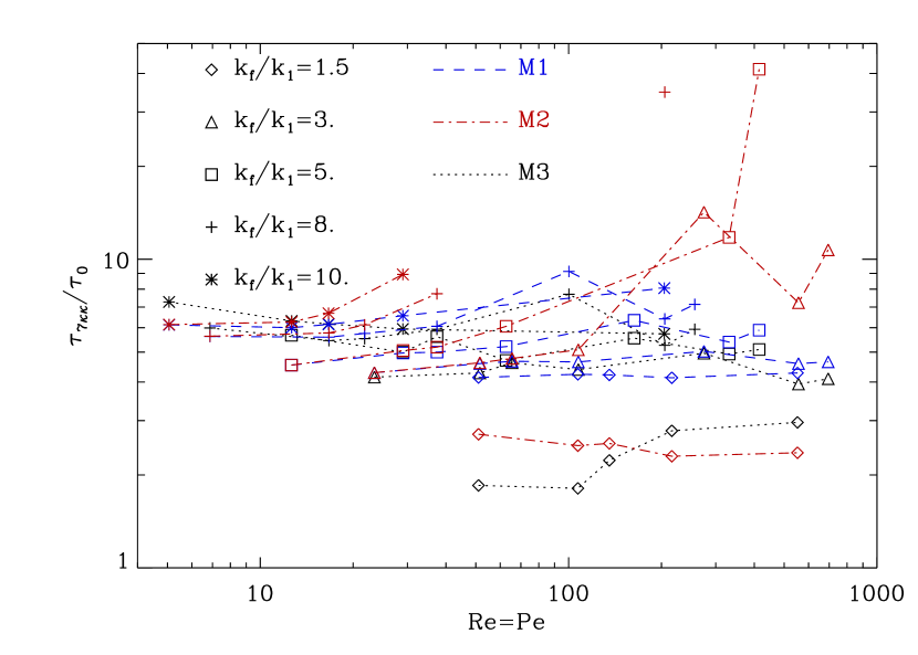
Figure 3: Comparison of relaxation timescales $\tau_{7\kappa\kappa}$ from methods M1 – M3. Negative results are not plotted. For explanations see Figure 2.

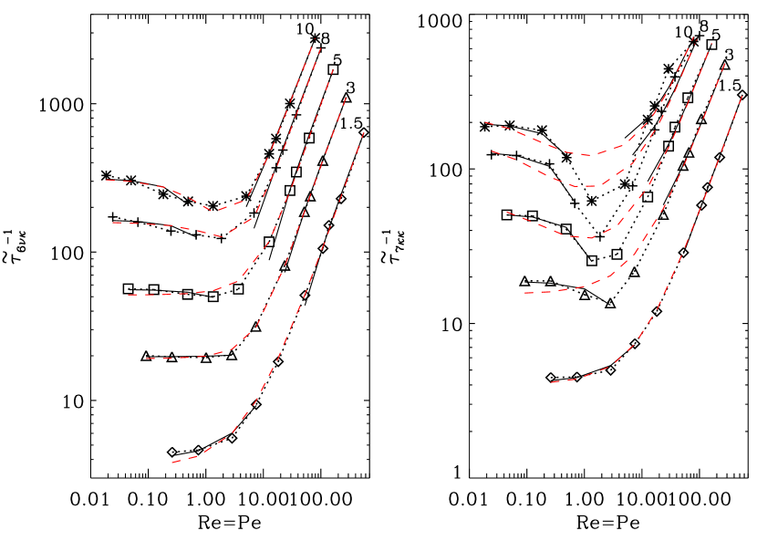
Figure 4: Relaxation times $\tilde{\tau}_{6\nu\kappa}$ (left) and $\tilde{\tau}_{7\kappa\kappa}$ (right), normalized to the viscous time $\tau_{\rm visc}$ as functions of $\mbox{\rm Re}=\mbox{\rm Pe}$, for different values of the scale separation $s$, indicated at the curves. Dotted lines with symbols: data from method M1; solid lines: linear fits according to (39), separately for low and high Re. Red dashed: approximation by (40) with parameters $C_{6}$, $C_{6}^{\prime}$, $C_{\nu\kappa}$, $C_{\nu\kappa}^{\prime}$ from a best fit, see Table 2.

Guided by these functional dependencies we hence propose as an alternative for (39)

$$\frac{1}{\tilde{\tau}_{6\nu\kappa}}=C_{6}s\mbox{\rm Re}+C_{\nu\kappa}+\frac{1}{C_{6}^{\prime}s\mbox{\rm Re}+C_{\nu\kappa}^{\prime}}\equiv F(\mbox{\rm Re}),$$ (40)

and analogously for $1/\tilde{\tau}_{7\kappa\kappa}$. This ansatz allows to model linear dependencies on Re both for small and large arguments, but with different coefficients:

$$F(\mbox{\rm Re}) \approx C_{6}s\mbox{\rm Re}+C_{\nu\kappa}\quad \mbox{for}\quad\mbox{\rm Re}\rightarrow\infty,$$ (41)

$$F(\mbox{\rm Re}) \approx\left(C_{6}-\frac{C_{6}^{\prime}}{{C_{\nu\kappa}^{\prime}}^{2}}\right)s\mbox{\rm Re}+C_{\nu\kappa}+\frac{1}{C_{\nu\kappa}^{\prime}}\quad \mbox{for}\quad\mbox{\rm Re}\rightarrow 0$$ (42)

where the slopes may well be different in sign. The constants in (40) were determined by a standard fitting procedure and are given in Table 2. For $\tilde{\tau}_{6\nu\kappa}$ the fit is surprisingly good throughout, whereas for $\tilde{\tau}_{7\kappa\kappa}$ this holds true merely for $s=1.5$. For larger scale separation the ansatz fails to model the pronounced minima at $\mbox{\rm Re}\approx 1$ visible in Figure 4 (right panel).

Table 2: Fit parameters of the scaling (40) for the results shown in Figure 4.

s	$C_{6}$	$C_{\nu\kappa}$	$10^{5}C_{6}^{\prime}$	$10^{3}C_{\nu\kappa}^{\prime}$	$C_{6}-C_{6}^{\prime}/{C_{\nu\kappa}^{\prime}}^{\!\!\!2}$	$C_{\nu\kappa}+1/C_{\nu\kappa}^{\prime}$	$C_{7}$	$C_{\kappa\kappa}$
1.5	0.86	-121.04	1.93	8.02	0.56	3.59	0.36	-0.20
3	1.39	-45.21	29.23	15.5	0.17	19.31	0.56	15.59
5	2.26	-177.86	3.47	4.36	0.44	51.31	0.75	36.01
8	3.06	-88.07	12.47	4.05	-4.54	158.69	0.84	76.88
10	3.50	-13.25	25.97	3.08	-23.86	311.38	0.74	121.19

The slopes for high Re, that is, $C_{6}$ and $C_{7}$, show a possible saturation with growing scale separation $s$, but the other coefficients do not. Hence, universality of the ansatz (40) with respect to scale separation is questionable.

4.2 Comparison of methods

Let us next compare the relaxation timescales $\tau_{6\nu\kappa}$ and $\tau_{7\kappa\kappa}$ obtained with the different methods in more detail.

4.2.1 Methods M1 and M3.

Figure 5 shows the ratio of the values of $\tau_{6\nu\kappa}$ and $\tau_{7\kappa\kappa}$ determined by either of the two methods in dependence on Re and $s$. The M3 values differ from the M1 ones by up to $\pm 30$ %. For $\tau_{6\nu\kappa}$ the deviations generally diminish with decreasing Re and with growing scale separation, falling beneath 10% for $s=8,10$. However, neither of these tendencies can be confirmed for $\tau_{7\kappa\kappa}$.

In view of the discussion in Sect. 2.6 it is satisfactory to find improving agreement between M1 and M3 with increasing scale separation for which our forced turbulence is more and more approaching the desired target of isotropic stationary turbulence.

Figure 5: Ratio of the values of $\tau_{6\nu\kappa}$ (left) and $\tau_{7\kappa\kappa}$ (right) determined by methods M1 and M3. Labels indicate the degree of scale separation $s$.

4.2.2 Methods M1 and M2.

As can be seen in Figure 6, for small scale separations $s=1.5,3,5$ the values of $\tau_{6\nu\kappa}$ from both methods coincide fairly. Deviations lie within errors. For large $s$, $s=8$, 10, however, we find the deviations grow with falling Re, being still within errors around $\mbox{\rm Re}=1$. We have to conclude that the neglect of $\overline{c\mbox{\boldmath$f$}{}}$ has its strongest effects for low Re and high $s$. In contrast, the differences between the $\tau_{7\kappa\kappa}$ values from methods M1 and M2 are much smaller, reaching a significant magnitude (exceeding errors ) only for the higher $s=8,10$ and $\mbox{\rm Re}\gtrsim 1$. A possible reason for this is insufficient numerical resolution.

Figure 6: Ratio of the values of $\tau_{6\nu\kappa}$ (left) and $\tau_{7\kappa\kappa}$ (right) determined by methods M1 and M2. Labels indicate the degree of scale separation $s$.

5 Comments and extensions

5.1 Alternative scaling

As an alternative to (38) one might consider

$$\frac{1}{\tau_{6\nu\kappa}}=C_{6}u_{\rm rms}k_{\rm f}+C_{\nu\kappa}(\nu+\kappa)\frac{k_{\rm f}^{2}}{2},\qquad\frac{1}{\tau_{7\kappa\kappa}}=C_{7}u_{\rm rms}k_{\rm f}+C_{\kappa\kappa}\kappa k_{\rm f}^{2}.$$ (43)

Then by multiplying with the dynamic time $\tau_{0}=(u_{\rm rms}k_{\rm f})^{-1}$ we arrive at

$$\frac{1}{\tilde{\tau}_{6\nu\kappa}}=C_{6}+\frac{C_{\nu\kappa}}{\mbox{\rm Re}},\qquad\frac{1}{\tilde{\tau}_{7\kappa\kappa}}=C_{7}+\frac{C_{\kappa\kappa}}{\mbox{\rm Pe}}.$$ (44)

where the normalization is now with respect to $\tau_{0}$. Figure 7 shows the same results as Figure 4, but now with the altered scaling. Again, a linear fit is viable on each curve, but only separately for low and high Re. The corresponding fit parameters can be found in Table 3. Unfortunately, an overall fit analogous to (40) does here not work satisfactorily.

Figure 7: Relaxation times $\tilde{\tau}_{6\nu\kappa}$ (left) and $\tilde{\tau}_{7\kappa\kappa}$ (right), normalized on the dynamical time $\tau_{0}$ as functions of $\mbox{\rm Re}^{-1}=\mbox{\rm Pe}^{-1}$, for different values of the scale separation $s$, indicated at the curves. Dotted lines with symbols: data from method M1; solid lines: linear fits according to (44), separately for low and high Re.

Table 3: Alternative fit parameters of the scaling (44) for the results shown in Figure 7.

s	small Re				large Re
	$C_{6}$	$C_{\nu\kappa}$	$C_{7}$	$C_{\kappa\kappa}$	$C_{6}$	$C_{\nu\kappa}$	$C_{7}$	$C_{\kappa\kappa}$
1.5	0.10	0.60	0.064	0.61	0.077	1.25	0.037	1.08
3	0.091	0.98	0.0025	0.94	0.14	0.55	0.061	0.97
5	0.052	1.37	-0.26	1.23	0.20	0.32	0.088	0.59
8	-2.21	2.29	-0.43	1.62	0.28	0.53	0.11	0.33
10	-5.84	3.39	-0.11	1.88	0.32	0.72	0.12	0.23

5.2 An Ogilvie approach for compressible hydrodynamics?

One could be tempted to treat the system (36) and (35) in the spirit of the Ogilvie approach quite analogously to what was shown in Sect. 2.1. In the ideal case and with $\overline{\bm{U}}=\bm{0}$, $\overline{H}=0$ we have for the fluctuating fields

$$\frac{\partial{\mbox{\boldmath$u$}{}}}{\partial\hskip 0.59998pt{t}} = -\big{(}\mbox{\boldmath$u$}{}\cdot\mbox{\boldmath$\nabla$}{}\mbox{\boldmath$u$}{}\big{)}^{\prime}-\mbox{\boldmath$\nabla$}{}h+{\mbox{\boldmath$f$}{}},$$ (45)

$$\frac{\partial{h}}{\partial\hskip 0.59998pt{t}} = -(\mbox{\boldmath$u$}{}\cdot\mbox{\boldmath$\nabla$}{}h)^{\prime}-c_{\rm s}^{2}\mbox{\boldmath$\nabla$}{}\cdot\mbox{\boldmath$u$}{},$$ (46)

and for the mean flux an analogue to (6), but with the term $-\overline{c\mbox{\boldmath$\nabla$}{}p}/\rho$ replaced by $-\overline{c\mbox{\boldmath$\nabla$}{}h}$. To close the system, an evolution equation for the quantity $\overline{c\mbox{\boldmath$\nabla$}{}h}$ seems hence to be indicated. From (3) and (46) we get

$$\frac{\partial{\,\overline{c\mbox{\boldmath$\nabla$}{}h}}}{\partial\hskip 0.59998pt{t}} = -c_{\rm s}^{2}\overline{c\mbox{\boldmath$\nabla$}{}\mbox{\boldmath$\nabla$}{}\cdot\mbox{\boldmath$u$}{}}-\overline{c\mbox{\boldmath$\nabla$}{}(\mbox{\boldmath$u$}{}\cdot\mbox{\boldmath$\nabla$}{}h)}-\overline{\mbox{\boldmath$\nabla$}{}h\mbox{\boldmath$\nabla$}{}\cdot(\mbox{\boldmath$u$}{}\overline{C})}-\overline{\mbox{\boldmath$\nabla$}{}h\cdot\mbox{\boldmath$\nabla$}{}(\mbox{\boldmath$u$}{}c)},$$ (47)

$$\frac{\partial{\left(\overline{c\mbox{\boldmath$\nabla$}{}h}\right)_{i}}}{\partial\hskip 0.59998pt{t}} = -\overline{\frac{\partial{h}}{\partial\hskip 0.59998pt{x_{i}}}\frac{\partial{u_{j}}}{\partial\hskip 0.59998pt{x_{j}}}}\overline{C}-\overline{u_{j}\frac{\partial{h}}{\partial\hskip 0.59998pt{x_{i}}}}\frac{\partial{\overline{C}}}{\partial\hskip 0.59998pt{x_{j}}}-c_{\rm s}^{2}\overline{c\frac{\partial{\,{}^{2}u_{j}}}{\partial\hskip 0.59998pt{x_{i}\partial x_{j}}}}-\;\mbox{third order terms},$$ (48)

where the second order correlation $\overline{c\,{\partial{{}^{2}u_{j}}/\partial{x_{i}\partial x_{j}}}}$ can only partly be expressed by $\overline{\cal F}_{i}$. The remaining parts could be modelled by a $\tau$ ansatz as used for the diffusion terms in Sect. 2.2, but note that here the “diffusivity” is $c_{\rm s}^{2}$ and we have no argument to consider the not properly modelled terms as small.

6 Conclusions

The main conclusion to be drawn from the present work is that the time scales used to model closure terms in the equations for the mean flux $\overline{\mbox{\boldmath$u$}{}c}$ and the mean square concentration $\overline{c^{2}}$ are nearly independent of Re for $\mbox{\rm Re}\geq 10$ and also nearly independent of the scale separation ratio for $k_{\rm f}/k_{1}\geq 3$. Expressed in terms of dynamical times, the resulting non-dimensional time scales can be referred to as Strouhal numbers whose values are around 3 for the $\overline{\mbox{\boldmath$u$}{}c}$ closure term and around 7 for the $\overline{c^{2}}$ closure term. The former value is in good agreement with earlier work using the $\tau$ approximation [5].

Equipped with this knowledge, we may now be better justified in using the closure hypotheses discussed here for the quantities $\overline{\mbox{\boldmath$u$}{}c}$ and $\overline{c^{2}}$. On the other hand, as explained in the present paper, it is quite clear that these closure hypotheses lack thorough justification [19]. One should therefore in future strive to find systematic discrepancies from the anticipated scalings. One example that we alluded to in the present paper is the inhomogeneous case in which the $\tau$ approach my break down. Future work in that direction seems now to be highly desirable, because in virtually all astrophysical applications the turbulence is inhomogeneous or at least anisotropic.

References

- [1] E. G. Blackman and G. B. Field. New Dynamical Mean-Field Dynamo Theory and Closure Approach. Physical Review Letters, 89(26):265007, 2002.
- [2] E. G. Blackman and G. B. Field. A new approach to turbulent transport of a mean scalar. Physics of Fluids, 15:L73–L76, 2003.
- [3] A. Brandenburg. The Inverse Cascade and Nonlinear Alpha-Effect in Simulations of Isotropic Helical Hydromagnetic Turbulence. Astrophys. J., 550:824–840, 2001.
- [4] A. Brandenburg, N. E. L. Haugen, and N. Babkovskaia. Turbulent front speed in the Fisher equation: Dependence on Damköhler number. Phys. Rev. E, 83(1):016304, 2011.
- [5] A. Brandenburg, P. J. Käpylä, and A. Mohammed. Non-Fickian diffusion and tau approximation from numerical turbulence. Physics of Fluids, 16:1020–1027, 2004.
- [6] A. Brandenburg and Å. Nordlund. Astrophysical turbulence modeling. Rep. Progr. Phys., 74(4):046901, 2011.
- [7] A. Brandenburg and K. Subramanian. Minimal tau approximation and simulations of the alpha effect. A&A, 439:835–843, 2005.
- [8] A. Brandenburg and K. Subramanian. Simulations of the anisotropic kinetic and magnetic alpha effects. Astronomische Nachrichten, 328:507, 2007.
- [9] P. Garaud and G. I. Ogilvie. A model for the nonlinear dynamics of turbulent shear flows. J. Fluid Mech., 530:145–176, 2005.
- [10] P. Garaud, G. I. Ogilvie, N. Miller, and S. Stellmach. A model of the entropy flux and Reynolds stress in turbulent convection. Mon. Not. R. Soc., 407:2451–2467, 2010.
- [11] A. Hubbard and A. Brandenburg. Memory Effects in Turbulent Transport. Astrophys. J., 706:712–726, 2009.
- [12] P. J. Käpylä and A. Brandenburg. Lambda effect from forced turbulence simulations. A&A, 488:9–23, 2008.
- [13] F. Krause and K.-H. Rädler. Mean-field magnetohydrodynamics and dynamo theory. Pergamon Press, Ltd., Oxford, 1980.
- [14] A. J. Liljeström, M. J. Korpi, P. J. Käpylä, A. Brandenburg, and W. Lyra. Turbulent stresses as a function of shear rate in a local disk model. Astron. Nachr., 330:92–99, 2009.
- [15] E. J. M. Madarassy and A. Brandenburg. Calibrating passive scalar transport in shear-flow turbulence. Phys. Rev. E, 82(1):016304, 2010.
- [16] N. Miller and P. Garaud. A Practical Model of Convective Dynamics for Stellar Evolution Calculations. In R. J. Stancliffe, G. Houdek, R. G. Martin, & C. A. Tout, editor, Unsolved Problems in Stellar Physics: A Conference in Honor of Douglas Gough, volume 948 of Am. Inst. Phys. Conf. Ser., pages 165–169, 2007.
- [17] H. K. Moffatt. Magnetic field generation in electrically conducting fluids. Cambridge University Press, Cambridge, England, 1978.
- [18] G. I. Ogilvie. On the dynamics of magnetorotational turbulent stresses. Mon. Not. R. Soc., 340:969–982, 2003.
- [19] K.-H. Rädler and M. Rheinhardt. Mean-field electrodynamics: critical analysis of various analytical approaches to the mean electromotive force. Geophys. Astrophys. Fluid Dyn., 101:117–154, 2007.
- [20] M. Rheinhardt and A. Brandenburg. Modeling spatio-temporal nonlocality in mean-field dynamos. Astron. Nachr., 333:80–86, 2012.
- [21] G. Rüdiger. Differential rotation and stellar convection. Sun and the solar stars. Akademie-Verlag, Berlin, 1989.
- [22] G. Rüdiger and R. Hollerbach. The magnetic universe: Geophysical and Astrophysical Dynamo Theory. Wiley-VCH, Berlin, 2004.
- [23] J. E. Snellman, A. Brandenburg, P. J. Käpylä, and M. J. Mantere. Verification of Reynolds stress parameterizations from simulations. Astron. Nachr., 332:883–888, 2011.
- [24] J. E. Snellman, P. J. Käpylä, M. J. Korpi, and A. J. Liljeström. Reynolds stresses from hydrodynamic turbulence with shear and rotation. A&A, 505:955–968, 2009.