Strong magnetic coupling of an inhomogeneous NV ensemble to a cavity

Abstract

We study experimentally and theoretically a dense ensemble of negatively charged nitrogen-vacancy centers in diamond coupled to a high $Q$ superconducting coplanar waveguide cavity mode at low temperature. The nitrogen-vacancy centers are modeled as effective spin one defects with inhomogeneous frequency distribution. For a large enough ensemble the effective magnetic coupling of the collective spin dominates the mode losses and inhomogeneous broadening of the ensemble and the system exhibits well resolved normal mode splitting in probe transmission spectra. We use several theoretical approaches to model the probe spectra and the number and frequency distribution of the spins. This analysis reveals an only slowly temperature dependent q-Gaussian energy distribution of the defects with a yet unexplained decrease of effectively coupled spins at very low temperatures below $100\text{\,}\mathrm{mK}$. Based on the system parameters we predict the possibility to implement an extremely stable maser by adding an external pump to the system.

I Introduction

Systems of spin ensembles coupled to a cavity mode are considered a promising physical realization for processing and storage of quantum information (Phillips et al., 2001), ultrasensitive high resolution magnetometers Taylor et al. (2008) or localized field probes. Collective magnetic coupling of a large ensemble to the field mode allows to reach the strong coupling regime, even if a single particle is hardly coupled. Implementations based on superconducting coplanar waveguide (CPW) resonators provide an interface of the spin ensemble with processing units for superconducting qubits. Here the spins can serve as a quantum memory or as a bridge to optical readout and communication (Verdú et al., 2009).

Different types of ensembles were proposed for this setup, ranging from clouds of ultracold atoms (Verdú et al., 2009) over polar molecules (Rabl et al., 2006) to solid state systems like rare-earth spin ensembles (Bushev et al., 2011) or color centers in diamond (Kubo et al., 2010; Amsüss et al., 2011). Here we focus on the negatively charged nitrogen-vacancy defects in diamond (NV). Those are naturally present in diamond but can also be readily engineered with very high densities, still maintaining long lifetimes and slow dephasing in particular at low temperatures of $T<$1\text{\,}\mathrm{K}$$. In the optical domain, they are extremely stable and very well studied since many years (Jelezko and Wrachtrup, 2006).

The magnetic properties of the relevant defect states can be conveniently modeled by effective independent spin 1 particles, where the effective local interaction of the electrons within the defect shifts the $(m_{S}=\pm 1)$ states with respect to the $m_{S}=0$ state Childress et al. (2006). On the one hand, this coupling provides the desired energy gap in the $3\text{\,}\mathrm{GHz}$ regime, but on the other hand, as a consequence of local variations of the crystal field, this shift exhibits a frequency distribution leading to an inhomogeneous broadening of the ensemble. The inhomogeneities are thought to be predominantly caused by crystal strain and excess nitrogen, which is not paired with a neighboring vacancy (Acosta et al., 2009).

While for a perfectly monochromatic ensemble of $N$ particles in a cavity, strong coupling simply requires an effective coupling $g_{\text{single}}\sqrt{N}$ larger than the cavity and spin decay rates, not only the width, but also the details of the inhomogeneous distribution are known to strongly influence the dynamic properties of the real world system (Houdré et al., 1996; Diniz et al., 2011; Kurucz et al., 2011). In particular a Gaussian or a Lorentzian distribution of equal half width, lead to different widths and magnitudes of the vacuum Rabi splitting. Only above a critical coupling strength the rephasing via common coupling to the cavity mode will prevent dephasing of the collective excitation and lead to a well resolved vacuum Rabi splitting.

In our theoretical studies of this system we use different approximation levels to analyze the central physical effects present in an inhomogeneously broadened system, as they are observed in the measurements. While many qualitative features can be readily understood from a simple, coupled damped oscillator model with an effective linewidth, a detailed understanding of the observed frequency shifts and coupling strengths in the experiments requires more sophisticated modeling of the energy distributions and dephasing mechanisms. In particular the observed temperature dependence relies on a finite temperature master equation treatment of a collective spin with proper dephasing terms. This is compared to the experimental values of up to ($N\approx 10^{12}$) particles as presented already in (Amsüss et al., 2011).

The paper is organized as follows: The general properties of the system are introduced in Sec. II. A first approximative treatment using coupled harmonic oscillators is shown in Sec. III.1. In Sec. III.2 we incorporate the inhomogeneous frequency distribution of the NVs via an extra decay of the polarization of the ensemble. In this context we also analyze the effects of thermal excitations in the spin ensemble and in the cavity. Finally, in Sec. III.3 we interpret our measurements using the resolvent formalism in order to extract the exact form of the inhomogeneity (Kurucz et al., 2011). The prospect of implementing a narrow bandwidth transmission line micro-maser using an inhomogeneously broadened ensemble is discussed in Sec. IV.

II General system properties and experimental implementation

The ground state of the NV center is a spin triplet $(S=1)$, where the $m_{S}=\pm 1$ states are split from the $m_{S}=0$ state by about $2.88\text{\,}\mathrm{GHz}$ at zero magnetic field (Acosta et al., 2009). In addition the degeneracy between the $m_{S}=\pm 1$ states is lifted due to the broken $C_{3v}$ symmetry. Applying a homogeneous magnetic field enables Zeeman tuning of the $m_{S}=\pm 1$ states, so that the $m_{S}=0\rightarrow\pm 1$ transitions can be tuned selectively into resonance with the CPW cavity.

Note that here the Zeeman tuning is also varying with the NV centers orientation relative to the applied field direction. In NV center ensembles all the four symmetry allowed orientations of the NV main axis are found and in general each orientation will enclose a different angle with the magnetic field and will be shifted by a different amount.

However, if the magnetic field direction is oriented within the (001) plane of the diamond, always two of four orientations exhibit the same angle with the field and at special angles all four are tuned by the same amount.

In general we therefore have to distinguish between the $m_{S}^{\text{I,II}}=\pm 1$ states of subensemble I and II. The Hamiltonian for one NV subensemble can be written as

$$\operatorname{H_{\text{NV}}}=\tilde{g}\mu_{B}\mathbf{B}\cdot\mathbf{S}+DS_{z}^{2}+E(S_{x}^{2}-S_{y}^{2}),$$ (1)

where the first term describes the Zeeman effect with $\tilde{g}=2$ for an NV center and $\mu_{B}$ being the Bohr magneton. The second term denotes the zero-field splitting with $D=$2.88\text{\,}\mathrm{GHz}$$ and typical strain-induced $E$ parameters of several MHz. The presence of non-zero E parameters in large NV ensembles causes a mixing of the pure Zeeman states for low magnetic field values which are denoted as $\ket{0,\pm}$. As the magnetic field amplitude is increased, the Eigenstates are again well approximated by pure Zeeman states.

The transition frequencies $\omega_{\pm}^{\text{I,II}}$ between the eigenstates $\ket{0}_{\text{I,II}}$ and $\ket{\pm}_{\text{I,II}}$ are depicted in Fig. 1(b).

II.1 Theoretical model

Assuming that only the transition $\ket{0}_{\text{I}}\rightarrow\ket{-}_{\text{I}}$ with frequency $\omega_{-}^{\text{I}}$ is in or close to resonance with the cavity mode, we can reduce the description of a single NV to a 2-level system. The effects caused by the presence of the far detuned $\ket{+}_{\text{I}}$ state can be included in a constant effective frequency shift as addressed in Sec. III.1. We thus approximate the composed system of cavity and ensemble with the Tavis-Cummings Hamiltonian

$$\operatorname{H}_{\text{TC}}=\omega_{c}a_{c}^{\dagger}a_{c}+\frac{1}{2}\sum^{N}_{j}\omega_{j}\sigma_{j}^{z}+\sum^{N}_{j}\left(g_{j}\sigma_{j}^{+}a_{c}+\text{H.c.}\right)\ ,$$ (2)

where $\hbar=1$. The first two terms describe the unperturbed energies of the cavity, with frequency $\omega_{c}$ and creation operator $a_{c}^{\dagger}$, and of the $N$ ensemble spins using the usual Pauli spin operators $\left(\left[\sigma_{i}^{+},\sigma_{j}^{-}\right]=\sigma_{i}^{z}\delta_{ij}\right)$. Each spin can have a different frequency $\omega_{j}$ which is statistically spread around the center frequency $\omega_{-}^{\text{I}}$. The third term describes the coupling to the cavity with individual strength $g_{j}$. Assuming that the ensemble spins are confined to a volume small compared to the wavelength, the ensemble will interact collectively with the mode. In the case of few excitations, the ensemble behaves like a harmonic oscillator which couples to the mode with the collective coupling strength $\Omega$. The collective coupling strength is given by $\Omega=\sqrt{\sum_{j}^{N}\left|g_{j}\right|^{2}}$ which for identical $g_{j}=g_{\text{single}}=g$ gives $\Omega=g\sqrt{N}$. To include the probe field of the cavity we add another term $\operatorname{H}_{p}=\mathrm{i}\left(\eta a_{c}^{\dagger}\mathrm{e}^{-\mathrm{i}\omega_{p}t}-\eta^{*}a_{c}\mathrm{e}^{\mathrm{i}\omega_{p}t}\right)$ to Eq. 2.

Effects of the coupling to a finite temperature bath are analyzed in Sec.III.2, where we study the master equation of the ensemble-cavity system.

For an ensemble with identical frequencies and coupling strengths we find that we can reach the regime of coherent oscillations between the cavity and the ensemble spins if the collective coupling $\Omega$ dominates the linewidth of the cavity $\kappa$ and the decay rate of the single spin $\gamma_{\text{hom}}$. This is commonly known as strong coupling regime. In case of an ensemble with inhomogeneous frequency distribution it is not immediately clear under which conditions we can observe the avoided crossing. Here we address the influence of the width and form of the inhomogeneous frequency distribution on the avoided crossing.

II.2 Experimental setup and parameters

The experimental set-up has been described already in detail in Amsüss et al. (2011) and is explained here only in brevity in the following. The heart of the experiment is a $\lambda/2$ superconducting coplanar waveguide (CPW) resonator with a center frequency of $2.7\text{\,}\mathrm{GHz}$ that is cooled down to $20\text{\,}\mathrm{mK}$ in a dilution refrigerator. In order to couple NV defect centers to the microwave field in the cavity, a (001)-cut single crystal diamond is placed in the middle of the resonator, where the oscillating magnetic field exhibits an antinode. A meander geometry of the resonator ensures that a large fraction of the magnetic mode volume is covered by spins. The high-pressure high-temperature diamond chosen in this setup contains an NV concentration of about $6$ ppm, which corresponds to an average separation of about $10\text{\,}\mathrm{nm}$.

A 2-axis Helmholtz coil configuration creates a homogeneous static magnetic field oriented with an arbitrary direction within the (001) plane of the diamond, which is at the same time parallel to the resonator chip surface. Since perpendicular magnetic field components with respect to the resonator surface would shift the resonance frequency of the cavity, great care was taken during the alignment of the set-up. With the diamond on top of the chip the cavity quality factor is $Q=3200$.

In a typical experiment, we first set the magnetic field direction and amplitude and then measure the microwave transmission through the cavity with a vector network analyzer.

III Cavity transmission spectra for inhomogeneous ensembles

As generic experiment to test and characterize the system properties we analyze the weak field probe transmission spectrum through the resonator in the weak field limit, where the number of excitations is negligible compared to the ensemble size. Hence, at least at low temperatures, we can largely ignore saturation effects and apply various simplified theoretical descriptions to extract the central system parameters. In fact as we deal with more than $N>10^{11}$ spins in a transition frequency range of about $10^{7}\text{\,}\mathrm{Hz}$, we have several thousand spins per Hz frequency range and up to a million spins within the homogeneous width of at least several kHz. Hence theoretical modelling as a collection of effective oscillators should provide an excellent model basis. This has to be taken with care at higher temperatures $k_{B}T\approx\hbar\omega_{c}$, when we have a significant fraction of the particles excited.

III.1 Coupled collective oscillator approximation

A photon that enters the cavity will be absorbed into a symmetric excitation of the ensemble spins with a weight given by the individual coupling strength. Subsequently the broad distribution of the spin frequencies induces a relative dephasing of this excitation so that the backcoupling to the cavity mode is suppressed. As spontaneous decay ($T_{1}\approx$44\text{\,}\mathrm{s}$$) is negligibly slow (Amsüss et al., 2011), the decay rate of the polarization of the ensemble is just proportional to this dephasing and thus the inhomogeneous width of the spins.

As the number of photons entering the ensemble is very small compared to $N$ in a first model, we simply approximate the ensemble as a harmonic oscillator with frequency $\omega_{a1}=\omega_{-}^{\text{I}}$ and an effective large width $\gamma$ that mimics the inhomogeneity. The ensemble oscillator is coupled to the cavity with frequency $\omega_{c}$ and decay rate $\kappa$.

This very simplified model already allows us to study the coupling dynamics of the collective energy levels of the broadened ensemble and the cavity mode, and in particular the avoided crossing of the energy levels, when the relative energies are varied.

To keep the model as simple as possible but still grasping the essential properties, the presence of the other offresonant spin ensembles at $\omega_{+}^{\text{I}}$, $\omega_{-}^{\text{II}}$ and $\omega_{+}^{\text{II}}$ is modelled by additional oscillators with frequency $\omega_{aj}$, ($j=2,3,4$) and equal decay rate $\gamma$.

For a small probe field injected into the cavity with the frequency $\omega_{p}$ the corresponding equations in a frame rotating with $\omega_{p}$ then read:

$$\frac{\mathrm{d}}{\mathrm{d}t}\left<a_{c}\right> =-\left(\kappa+\mathrm{i}\Delta_{c}\right)\left<a_{c}\right>-\mathrm{i}g\sum_{j=1}^{4}N_{j}\left<\sigma_{j}^{-}\right>+\eta$$ (3)

$$\frac{\mathrm{d}}{\mathrm{d}t}\left<\sigma_{j}^{-}\right> =-\left(\frac{\gamma}{2}+\mathrm{i}\Delta_{aj}\right)\left<\sigma_{j}^{-}\right>-\mathrm{i}g\left<a_{c}\right>\ ,$$ (4)

with probe amplitude $\eta$, $\Delta_{c}=\omega_{c}-\omega_{p}$ and $\Delta_{aj}=\omega_{aj}-\omega_{p}$. From Eqs. 3 and 4 we can calculate the steady state field in the cavity $\left<a_{c}\right>_{\text{st}}$, which can be written as

$$\left<a_{c}\right>_{\text{st}}=\frac{\eta}{\kappa+\Gamma_{a}+\mathrm{i}\left(\Delta_{c}-U_{a}\right)+\frac{g^{2}N_{1}}{\gamma/2+\mathrm{i}\Delta_{a1}}}\ ,$$ (5)

where

$$\Gamma_{a}=\sum_{j=2}^{4}\frac{g^{2}N_{j}\gamma/2}{\left(\gamma/2\right)^{2}+\Delta_{aj}^{2}}\ \ \text{and}\ \ U_{a}=\sum_{j=2}^{4}\frac{g^{2}N_{j}\Delta_{aj}}{\left(\gamma/2\right)^{2}+\Delta_{aj}^{2}}\ .$$ (6)

In the absence of the offresonant levels ($N_{2}=N_{3}=N_{4}=0$) we recover the situation, where for $\omega_{a1}=\omega_{c}$ and $g\sqrt{N_{1}}>(\gamma/2-\kappa)/2$ we find two normal modes split by $2\sqrt{g^{2}N_{1}-(\gamma/2-\kappa)^{2}/4}$. The offresonant transitions make the situation more complex. As it can be seen in Eq. 5, they induce a shift $U_{a}$ of the cavity frequency and increase the decay rate of the cavity by $\Gamma_{a}$. Both, shift and additional decay rate, depend on the probe frequency $\omega_{p}$. For the parameters in our measurement we find that $\Gamma_{a}$ is negligible compared to $\kappa$. We further approximate $U_{a}$ by setting $\omega_{p}=\omega_{c}$ (as the scan range of $\omega_{p}$ around $\omega_{c}$ is small compared to $\omega_{aj}$ ($j=2,3,4$)). We obtain the model of two coupled oscillators, where one of them has been shifted by the offresonant transitions. As a function of $\omega_{p}$ and $\omega_{a1}$ (tuned by the magnetic field), $\left|\left<a_{c}\right>_{\text{st}}\right|^{2}$ shows an avoided crossing. Although the offresonant transitions are shifted by the magnetic field as well, the effect in $U_{a}$ is negligibly small, so that we assume that $U_{a}$ is constant.

We show the measured signal at the avoided crossing in Fig. 1(a). By fitting $\left|\left<a_{c}\right>_{\text{st}}\right|^{2}$ to the normal mode splitting we can deduce the inhomogeneous width $\gamma$ and the effective coupling $g\sqrt{N}$. The $Q$ factor of our cavity corresponds to $\kappa/(2\pi)=$0.4\text{\,}\mathrm{MHz}$$, then $2\kappa$ is the full width at half maximum (FWHM) of the cavity resonance. An exemplary fit result is shown in Fig. 1(c). We have included a linear term in the fit to account for a background in the data. In Fig. 1(d) we plot $\left|\left<a_{c}\right>_{\text{st}}\right|^{2}$ using the obtained parameters.

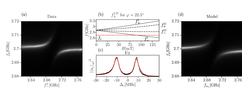
Figure 1: (a) (Color online) Measured transmission as a function of $f_{-}^{\text{I}}=\omega_{-}^{\text{I}}/(2\pi)$ tuned by the magnetic field and pump frequency $f_{p}=\omega_{p}/(2\pi)$. (b) Transition frequencies $f_{\pm}^{\text{I,II}}=\omega_{\pm}^{\text{I,II}}/(2\pi)$ as a function of the magnetic field for a field angle of $\varphi=22.5^{\mathrm{\SIUnitSymbolDegree}}$. The frequency of the cavity $f_{c}=\omega_{c}/\left(2\pi\right)$ is denoted by the (red) dashed line. (c) Fit of $\left|\left<a_{c}\right>_{\text{st}}\right|^{2}$ to the transmitted signal close to the resonance. We obtain the decay rate $\gamma=$10.92\text{\,}\mathrm{MHz}$$. (d) $\left|\left<a_{c}\right>_{\text{st}}\right|^{2}$ as a function of $f_{a_{1}}$ and $f_{p}$ incorporating the parameters obtained from the fit.

From the fit we deduce a decay rate $\gamma=$10.92\text{\,}\mathrm{MHz}$$ of the ensemble oscillator and an effective coupling of $g\sqrt{N}=$9.51\text{\,}\mathrm{MHz}$$. To demonstrate the effect of the ensemble oscillator width $\gamma$ on the normal mode splitting, we plot $\left|\left<a_{c}\right>_{\text{st}}\right|^{2}$ for $\omega_{c}-U_{a}=\omega_{a1}$ and different values of $\gamma$ in Fig. 2.

Treating the ensemble as a broad harmonic oscillator with decay rate $\gamma$ corresponds to the assumption that the frequency distribution of the real ensemble is a Lorentzian distribution, given that all spins couple with equal strength Kurucz et al. (2011).

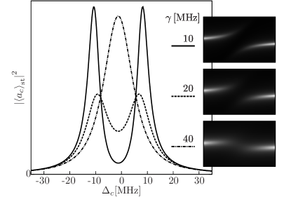
Figure 2: Simulation of the normal mode splitting at resonance ($\omega_{c}-U_{a}=\omega_{a1}$) for different values of $\gamma$. Finally for large values of $\gamma$ the doublet is not resolved any more and the avoided crossing (sketched on the right) becomes blurred.

III.2 Polarization decay and collective coupling at finite temperature

Despite cooling to very low temperatures is possible in the experiments, it is still important and instructive to study the role of thermal excitations in the system. In contrast to previous models based on virtually zero $T$ atomic ensembles, the NV centers are in thermal contact with the chip at small but finite $T$. We will now investigate how sensitive the system reacts on thermal fluctuations.

At this point we include any shifts caused by the off-resonant ensembles in an effective detuning and concentrate on the collective coupling between the cavity at $\omega_{c}$ and the near resonant ensemble centered around $\omega_{-}^{\text{I}}$. For simplicity we assume equal coupling $g$ for all spins to get

$$\operatorname{\tilde{H}}_{\text{TC}}=\omega_{c}a_{c}^{\dagger}a_{c}+\frac{1}{2}\omega_{-}^{\text{I}}\sum^{N}_{j}\sigma_{j}^{z}+g\sum^{N}_{j}\left(\sigma_{j}^{+}a_{c}+\text{H.c.}\right)\ .$$ (7)

The effects of unequal coupling of the spins is addressed in Braun et al. (2011).

To include thermal excitations of the mode and the ensemble we have to add standard Liouvillian terms to the dynamics and study the corresponding master equation of the reduced cavity ensemble system Carmichael (1993), where the inhomogeneous width of the ensemble is still simply approximated by an effective dephasing term $\gamma_{p}$ for the polarization. In this model decay $\gamma_{\text{hom}}$ and dephasing $\gamma_{p}$ are described by separate quantities, which already should improve the model. The master equation reads

$$\frac{\mathrm{d}}{\mathrm{d}t}\rho=\frac{1}{\mathrm{i}}\left[\operatorname{\tilde{H}}_{\text{TC}}+\operatorname{H}_{p},\rho\right]+\mathcal{L}\left[\rho\right]\ ,$$ (8)

where

$$\mathcal{L}\left[\rho\right]=\kappa\left(\mathrm{bar}{n}\left(T,\omega_{c}\right)+1\right)\left(2a_{c}\rho a_{c}^{\dagger}-a_{c}^{\dagger}a_{c}\rho-\rho a_{c}^{\dagger}a_{c}\right)$$

$$+\kappa\mathrm{bar}{n}\left(T,\omega_{c}\right)\left(2a_{c}^{\dagger}\rho a_{c}-a_{c}a_{c}^{\dagger}\rho-\rho a_{c}a_{c}^{\dagger}\right)$$

$$+\frac{\gamma_{\text{hom}}}{2}\left(\mathrm{bar}{n}\left(T,\omega_{-}^{\text{I}}\right)+1\right)\sum_{j=1}^{N}\left(2\sigma_{j}^{-}\rho\sigma_{j}^{+}-\sigma_{j}^{+}\sigma_{j}^{-}\rho-\rho\sigma_{j}^{+}\sigma_{j}^{-}\right)$$

$$+\frac{\gamma_{\text{hom}}}{2}\mathrm{bar}{n}\left(T,\omega_{-}^{\text{I}}\right)\sum_{j=1}^{N}\left(2\sigma_{j}^{+}\rho\sigma_{j}^{-}-\sigma_{j}^{-}\sigma_{j}^{+}\rho-\rho\sigma_{j}^{-}\sigma_{j}^{+}\right)$$

$$+\frac{\gamma_{p}}{2}\sum_{j=1}^{N}\left(\sigma_{j}^{z}\rho\sigma_{j}^{z}-\rho\right)\ .$$ (9)

The first two lines of Eq. 9 describe the coupling of the cavity to the bath, while the next two lines include the coupling of the ensemble to the bath. The number of thermal excitations at temperature $T$ and frequency $\omega$ is denoted by $\mathrm{bar}{n}\left(T,\omega\right)$. The term in the last line introduces nonradiative dephasing at a rate $\gamma_{p}$ of the spins and thereby models the inhomogeneity.

Based on the master equation we can derive a hierarchic set of equations for various system expectation values starting with

$$\frac{\mathrm{d}}{\mathrm{d}t}\left<a_{c}\right> =\operatorname{Tr}\{a_{c}\frac{\mathrm{d}}{\mathrm{d}t}\rho\}$$

$$=-\left(\kappa+\mathrm{i}\Delta_{c}\right)\left<a_{c}\right>-\mathrm{i}gN\left<\sigma_{i}^{-}\right>+\eta\ ,$$ (10)

$$\frac{\mathrm{d}}{\mathrm{d}t}\left<\sigma_{i}^{-}\right> =-\left(\frac{\gamma_{\text{hom}}}{2}+\gamma_{\text{hom}}\mathrm{bar}{n}\left(T,\omega_{-}^{\text{I}}\right)+\gamma_{p}+\mathrm{i}\Delta_{-}^{\text{I}}\right)\left<\sigma_{i}^{-}\right>$$

$$+\mathrm{i}g\left<\sigma_{i}^{z}a_{c}\right>\ ,$$ (11)

$$\frac{\mathrm{d}}{\mathrm{d}t}\left<\sigma_{i}^{z}\right> =-\mathrm{i}2g\left(\left<\sigma_{i}^{+}a_{c}\right>-\left<\sigma_{i}^{-}a_{c}^{\dagger}\right>\right)-\gamma_{\text{hom}}\left(\left<\sigma_{i}^{z}\right>+1\right)$$

$$-2\gamma_{\text{hom}}\mathrm{bar}{n}\left(T,\omega_{-}^{\text{I}}\right)\left<\sigma_{i}^{z}\right>\ ,$$ (12)

which also includes equations for $\left<a_{c}\sigma_{i}^{+}\right>$, $\left<a_{c}\sigma_{i}^{z}\right>$, $\left<\sigma_{i}^{+}\sigma_{j}^{-}\right>$, $\left<a_{c}^{\dagger}a_{c}\right>$, $\left<a_{c}\sigma_{i}^{-}\right>$, $\left<a_{c}^{\dagger}a_{c}^{\dagger}\right>$, $\left<\sigma_{i}^{-}\sigma_{j}^{-}\right>$, $\left<\sigma_{i}^{z}\sigma_{j}^{+}\right>$, $\left<\sigma_{i}^{z}\sigma_{j}^{z}\right>$ and $\left<a_{c}^{\dagger}a_{c}\sigma_{i}^{z}\right>$. In order to truncate the system higher order terms in the equations are expanded in a well defined way (Kubo, 1962), then higher order cumulants are neglected (Meiser et al., 2009; Henschel et al., 2010). The equations again are written in a frame rotating with the cavity probe frequency $\omega_{p}$. Despite the inhomogeneous broadening, which is included by the nonradiative dephasing of the spins, we assume that all spins are equal so that we only have to include the equations for one spin $i$ and pairs $i,j$ Meiser et al. (2009). This set of equations can be integrated numerically to study the dynamics of the coupled system. We note that when we fix $\left<\sigma_{i}^{z}\right>=-1$ we immediately arrive at the model discussed in Sec. III.1 with $\gamma=\gamma_{\text{hom}}+2\gamma_{p}$.

In our experiment we measure the avoided crossing for different temperatures of the environment and compare it to the results of our model. First we note that the steady state of the inversion as a function of the temperature $\left<\sigma_{i}^{z}(T)\right>_{\text{st}}$ can be written as (Bushev et al., 2011)

$$\left<\sigma_{i}^{z}(T)\right>_{\text{st}} =\frac{1}{1+2\mathrm{bar}{n}\left(T,\omega_{-}^{\text{I}}\right)}\left<\sigma_{i}^{z}(T=0)\right>_{\text{st}}$$

$$=\tanh{\left(\frac{\hbar\omega_{i}}{2k_{B}T}\right)}\left<\sigma_{i}^{z}(T=0)\right>_{\text{st}}\ .$$ (13)

For higher temperatures $\left<\sigma_{i}^{z}(T)\right>_{\text{st}}$ is reduced and therefore the effective number of NVs that take part in the dynamics. In the model equations this is represented by the last term in Eq.11 for the polarization involving $\left<a_{c}\sigma_{i}^{z}\right>$, which leads to a cutoff for the coupling at higher $T$. As a zero field approximation we thus write

$$\Omega(T)=g\sqrt{N\tanh{\left(\frac{\hbar\omega^{\text{I}}_{-}}{2k_{B}T}\right)}}\ ,$$ (14)

where we replaced $\omega_{i}$ by the center frequency $\omega^{\text{I}}_{-}$. Equation (14) should give an approximate description of the reduction of the Rabi splitting with increasing temperature.

This treatment however neglects the presence of the $m_{S}=+1$ state which will also be populated with increasing $T$. Including this level and assuming $\mathrm{bar}{n}\left(T,\omega_{+}^{\text{I}}\right)\approx\mathrm{bar}{n}\left(T,\omega_{-}^{\text{I}}\right)$ we find the population difference between the $m_{S}=0$ and $m_{S}=-1$ state to be

$$\frac{N_{-1}(T)}{N}-\frac{N_{0}(T)}{N}=-\frac{1}{1+3\mathrm{bar}{n}\left(T,\omega_{-}^{\text{I}}\right)}\ .$$ (15)

This suggests

$$\tilde{\Omega}(T)=g\sqrt{\frac{N}{1+3\mathrm{bar}{n}\left(T,\omega_{-}^{\text{I}}\right)}}$$ (16)

to be a better description for the temperature dependence of the coupling.

In a second step we integrate the whole hierarchic set of equations numerically for $\omega_{c}=\omega_{-}^{\text{I}}$ and varying pump frequency $\omega_{p}$. From $\left|\left<a_{c}\right>_{\text{st}}\right|^{2}\left(\omega\right)$ we determine the Rabi splitting for different temperatures from which we obtain the collective coupling. This can be compared to our measurements and the approximations in Eqs. 14 and  16.

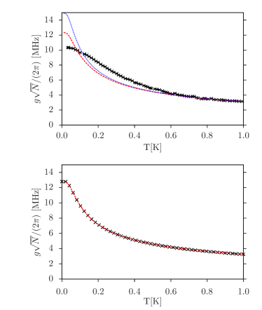
Figure 3: (Color online) (a) Collective coupling strength obtained from our measurements for different temperatures (black markers) and $\Omega(T)=a_{0}\left[\tanh{\left(\hbar\omega^{\text{I}}_{-}/(2k_{B}T)\right)}\right]^{1/2}$ (red dashed line), where $a_{0}$ was chosen to match the high temperature behavior. Including the $m_{S}=+1$ state via Eq. 16 gives the result denoted by the blue dotted line. (b) Collective coupling strength determined from the results of the numerical integration of the coupled equations with $g\sqrt{N}=a_{0}$ ($a_{0}$ determined from (a), black markers) and $\Omega(T)$ (red dashed line).

In Fig. 3(a) we show that the measured coupling strength is in disagreement with the Eq. 14, which is most significant for very low temperatures. Both functions Eq. 14 and Eq. 16 fail to capture the behavior for low temperatures. The disagreement is even more pronounced as we include the effect of the $m_{S}=+1$ state. So far we found no definite explanation for the disagreement. However, one possible explanation would be that for low temperatures not all defects are “active“. As temperature increases, more NVs become available but at the same time the number of NVs taking part in the dynamics is proportional to $\tanh{\left(\hbar\omega^{\text{I}}_{-}/(2k_{B}T)\right)}$.

The collective coupling strength determined from the numerical integration of the coupled equations, shown in Fig. 3(b), exactly follows Eq. 14. This shows that the assumption $\Omega(T)\propto\left<\sigma_{i}^{z}(T)\right>_{\text{st}}$ is reasonable. However, the almost constant value of the coupling strength $\Omega(T)$ found in the experimental data for very low $T$ cannot be explained in the above theoretical model. As possible explanations one might think of a reduced thermal excitation probability due to spin-spin coupling or an effective reduction of active NV centers close to zero temperature. Interestingly the same behavior is also found in measurements of dispersive shift of the cavity mode as a function of temperature by the offresonant spin ensemble at zero magnetic field.

III.3 Detailed modeling and reconstruction of inhomogeneous distributions

The simplified model descriptions discussed above in Secs. III.1 and  III.2 provided for an analytically tractable and qualitatively correct description of the effect of an inhomogeneous broadening of the ensemble. This also allows to get a fairly good estimate for the total width of the frequency distribution of the ensemble. However, such an effective width model inherently is connected to the assumption of a Lorentzian shape of the ensemble frequency distribution. In actual crystals such an assumption is not obvious and other distributions of local field variations and strain distributions are possible as well.

To obtain more accurate information about the distribution we will now use an improved model based on the resolvent formalism to treat the coupling between a central oscillator (the mode) and the spin degrees of freedom (Kurucz et al., 2011; Cohen-Tannoudji et al., 1992). Here each frequency class of spins is treated individually. For low temperatures virtually all spins are in the $m_{S}=0$ state, i.e. the lower state of our effective two-level system and their excitation properties can be approximated by a frequency distributed set of oscillators (Holstein-Primakoff approximation).

We define creation and annihilation operators for the corresponding ensemble oscillators representing a subclass of two-level systems with equal frequency via

$$\sigma^{z}_{j}=-1+2a_{j}^{\dagger}a_{j}\quad\text{and}\quad\sigma_{j}^{+}=a_{j}^{\dagger}\sqrt{1-a_{j}^{\dagger}a_{j}}\approx a_{j}^{\dagger}\ .$$ (17)

The approximation in Eq. 17 is justified as long as the number of excitations in each ensemble is much smaller than the number of spins in this energy region. In our experimental setup this is very well justified and we thus obtain the unperturbed part of the Hamiltonian as

$$\operatorname{H}_{0}^{\prime} =\omega_{c}a_{c}^{\dagger}a_{c}+\sum^{N}_{j}\omega_{j}a_{j}^{\dagger}a_{j}\ ,$$ (18)

and the interaction term

$$\operatorname{V}^{\prime}=\sum^{N}_{j}\left(g_{j}a_{j}^{\dagger}a_{c}+g^{*}_{j}a_{j}a^{\dagger}_{c}\right)\ ,$$ (19)

which constitute $\operatorname{H}^{\prime}=\operatorname{H}_{0}^{\prime}+\operatorname{V}^{\prime}$. In this section we account for the decay of cavity excitations and the spontaneous decay of the spins by introducing nonzero imaginary parts of the corresponding transition frequencies $\operatorname{Im}\omega_{c}=-\kappa$ and $\operatorname{Im}\omega_{j}=-\frac{1}{2}\gamma_{\text{hom}}$ and the resolvent of the Hamiltonian $\operatorname{H}^{\prime}$ is defined as $\operatorname{G}\left(z\right)=1/\left(z-\operatorname{H}^{\prime}\right)$.

Let us consider the state $\ket{\varphi_{c}}=\ket{1_{c},0,\dots,0}$ where we have one photon in the cavity and no excitation in the ensemble.

The matrix element of the resolvent $\operatorname{G}_{cc}\left(z\right)=\bra{\varphi_{c}}\operatorname{G}\left(z\right)\ket{\varphi_{c}}$ can be written as

$$G_{cc}\left(z\right)=\frac{1}{z-E_{c}-R_{cc}\left(z\right)}\ ,$$ (20)

where we define the matrix element of the level shift operator

$$R_{cc}\left(z\right) =V^{\prime}_{cc}+\sum_{i\neq c}V^{\prime}_{ci}\frac{1}{z-E_{i}}V^{\prime}_{ic}$$

$$+\sum_{i\neq c}\sum_{j\neq c}V^{\prime}_{ci}\frac{1}{z-E_{i}}V^{\prime}_{ij}\frac{1}{z-E_{j}}V^{\prime}_{jc}+\dots\ ,$$ (21)

where $V^{\prime}_{kl}=\bra{\varphi_{k}}\operatorname{V}^{\prime}\ket{\varphi_{l}}$ and $E_{c}=\bra{\varphi_{c}}\operatorname{H}^{\prime}_{0}\ket{\varphi_{c}}$. States $\ket{\varphi_{i}}$ with $i\neq c$ are states where the excitation is absorbed in the ensemble spin $i$. We note that $V^{\prime}_{cc}=0$ and that $V^{\prime}_{ij}=0$ for $i,j\neq c$ since our Hamiltonian does not include spin-spin interaction. Only the second term in Eq. 21 remains and we can write

$$R_{cc}\left(z\right)=\sum_{i\neq c}\frac{\left|g_{i}\right|^{2}}{z-E_{i}}\ .$$ (22)

Introducing the coupling density profile $\rho\left(\omega\right)\equiv\sum_{j}\left|g_{j}\right|^{2}\delta\left(\omega-\operatorname{Re}\omega_{j}\right)$ as it is done in Kurucz et al. (2011) leads to

$$R_{cc}\left(z\right)=\int\frac{\rho\left(\omega\right)}{z-\omega+\frac{\mathrm{i}}{2}\gamma_{\text{hom}}}\mathrm{d}\omega\ .$$ (23)

Approaching the branch cut at $\omega-\frac{\mathrm{i}}{2}\gamma_{\text{hom}}$ we write

$$\lim_{\eta\rightarrow 0^{+}}R_{cc}\left(\omega-\frac{\mathrm{i}}{2}\gamma_{\text{hom}}\pm\mathrm{i}\eta\right)=R^{\pm}_{cc}\left(\omega-\frac{\mathrm{i}}{2}\gamma_{\text{hom}}\right)\ .$$ (24)

Using $\lim_{\eta\rightarrow 0^{+}}\frac{1}{x\pm\mathrm{i}\eta}=\mathcal{P}\frac{1}{x}\mp\mathrm{i}\pi\delta\left(x\right)$, where $\mathcal{P}$ denotes the Cauchy principal value, we find

$$R^{\pm}_{cc}\left(\omega-\frac{\mathrm{i}}{2}\gamma_{\text{hom}}\right)=\mathcal{P}\int\frac{\rho\left(\omega^{\prime}\right)}{\omega-\omega^{\prime}}\mathrm{d}\omega^{\prime}\mp\mathrm{i}\pi\rho\left(\omega\right)\ .$$ (25)

Experimentally we probe the transmission of a weak probe signal amplitude through the cavity as a function of frequency. The position and shape of the weak field transmission resonances can be determined from the complex poles of $G^{+}_{cc}\left(\omega\right)=1/\left(\omega-\omega_{c}-R^{+}_{cc}\left(\omega\right)\right)$, which contains the spin energy distribution on the right hand side. We can therefore extract information about the coupling density $\rho\left(\omega\right)=-\frac{1}{\pi}\operatorname{Im}R^{+}_{cc}\left(\omega-\frac{\mathrm{i}}{2}\gamma_{\text{hom}}\right)$ by carefully analyzing the measured transmission spectrum. For small $\gamma_{\text{hom}}$ the reconstruction simplifies to:

$$\rho\left(\omega\right)\approx-\frac{1}{\pi}\operatorname{Im}R^{+}_{cc}\left(\omega\right)+\frac{1}{2\pi}\frac{\partial\operatorname{Re}R^{+}_{cc}\left(\omega\right)}{\partial\omega}\gamma_{\text{hom}}\ ,$$ (26)

where $\operatorname{Im}R_{cc}^{+}\left(\omega-\frac{\mathrm{i}}{2}\gamma_{\text{hom}}\right)$ is expanded in a Taylor series around $\gamma_{\text{hom}}=0$. We can therefore directly use the frequency distribution of the transmitted signal $\left|\left<a_{c}\right>_{\text{st}}\right|^{2}$ via

$$\left|\left<a_{c}\right>_{\text{st}}\right|^{2} \propto\left|G^{+}_{cc}\left(\omega,\omega_{c}\right)\right|^{2}$$

$$=\frac{1}{\left(\omega-\omega_{c}-\operatorname{Re}R^{+}_{cc}\left(\omega\right)\right)^{2}+\left(\kappa+\operatorname{Im}R^{+}_{cc}\left(\omega\right)\right)^{2}}$$ (27)

to determine $R^{+}_{cc}\left(\omega\right)$. Let us point out here that Eq. 27 exhibits a Lorentzian shape as a function of $\omega_{c}$ with peak position $\omega-\operatorname{Re}R^{+}_{cc}\left(\omega\right)$ and peak width of $2\left(\kappa+\operatorname{Im}R^{+}_{cc}\left(\omega\right)\right)$. After extraction of the relevant parameters which determine $R^{+}_{cc}\left(\omega\right)$ from the measured spectra, we can simply use Eq. 26 to find the coupling density $\rho\left(\omega\right)$. Assuming that all spins are coupled with equal strength, one finds that $\rho\left(\omega\right)=g^{2}N\mathcal{M}\left(\omega\right)$ where $\mathcal{M}\left(\omega\right)$ is the frequency distribution of the spins.

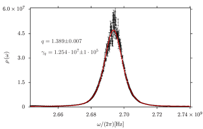
Figure 4: (Color online) Coupling density of the ensemble determined from an exemplary transmission measurement at $T=$20\text{\,}\mathrm{mK}$$. The errorbars are calculated from the uncertainties in $R_{cc}^{+}\left(\omega\right)$ which we obtain from fitting Eq. 27 to the data. We fit the q-Gaussian (red) in Eq. 28 to the coupling density to determine the width and the behavior of the tails of the distribution.

The shape of the coupling density, i.e. the frequency distribution of the spins, plays an important role in the cavity ensemble interaction Kurucz et al. (2011); Diniz et al. (2011). If the coupling density falls off sufficiently fast with distance from the center, the width of the Rabi peaks will decrease with increasing collective coupling strength $g\sqrt{N}$. For the spin frequency distribution, the limiting case is the Lorentzian coupling density profile, for which the width of the Rabi peaks is independent of $g\sqrt{N}$ (Diniz et al., 2011). Any distribution falling of faster than $1/\omega^{2}$ will provide a decrease of the width of the Rabi peaks. Moreover, knowing the coupling density gives us the opportunity to study the transmission through the cavity for different parameter ranges via Eq. 20.

To determine $\rho\left(\omega\right)$ the raw data have to be rearranged, since in the experiment we cannot simply vary $\omega_{c}$ but we shift the center frequency of the spins by a magnetic field. We therefore shift each scan by $\omega_{c}-\omega_{-}^{\text{I}}\left(B\right)$ to obtain fixed ensemble frequencies and tuning of the cavity frequency. As the only significant quantity is the detuning between the cavity and the ensemble this does not change the dynamics. For fixed $\omega$ we fit a Lorentzian to $\left|G^{+}_{cc}\left(\omega,\omega_{c}\right)\right|^{2}$ to determine $R^{+}_{cc}\left(\omega\right)$ in order to calculate $\rho\left(\omega\right)$. We plot an exemplary result for $\rho\left(\omega\right)$ in Fig. 4. To determine the behavior of the tails of the distribution we fit the function

$$L\left(\omega\right)=b+I\left[1-\left(1-q\right)\frac{\left(\omega-\omega_{0}\right)^{2}}{a}\right]^{\frac{1}{1-q}}\ ,$$ (28)

to the data. $L\left(\omega\right)$ is related to the q-Gaussian, a Tsallis distribution. The dimensionless parameter $1<q<3$ determines how fast the tails of the distribution fall off, while $a$ is related to the width. The actual width (FWHM) is given by $\gamma_{q}=2\sqrt{\frac{a\left(2^{q}-2\right)}{2q-2}}$. For $q\rightarrow 1$ we recover a Gaussian distribution, while for $q=2$ we find a Lorentzian distribution. The wings fall of as $1/\omega^{2/(q-1)}$.

From the fit in Fig. 4 we find values for $q=1.389\pm 0.007$ and $\gamma_{q}/(2\pi)=$(12.54\pm 0.10)\text{\,}\mathrm{MHz}$$. The temperature during the measurement was $20\text{\,}\mathrm{mK}$.

The same analysis is performed for data measured for $T=$20-1000\text{\,}\mathrm{mK}$$, see Fig 5(a). The fitted curves are not shown.

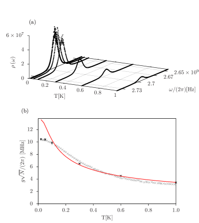
Figure 5: (Color online) In (a) we show the coupling density for different temperatures. The $q$-parameter and width $\gamma_{q}$ of the coupling density do not change significantly with increasing temperature. The coupling $g\sqrt{N}=\left(\int\rho\left(\omega\right)\mathrm{d}\omega\right)^{1/2}$ is reduced, as can be seen in (b). The red line shows $\Omega(T)=a_{0}\left[\tanh{\left(\hbar\omega^{\text{I}}_{-}/(2k_{B}T)\right)}\right]^{1/2}$ with $a_{0}$ chosen to match the high temperature limit of the data (black markers). To compare $\Omega(T)$ with our previous results determined directly from the splitting we plot the data already shown in Fig. 3 using grey markers.

For the resulting coupling densities we find almost no change in the width or the q-parameter. However, with increasing temperature $\int\rho\left(\omega\right)\mathrm{d}\omega=g^{2}N$ is reduced, as can be seen in Fig. 5(b). The resulting coupling strength is in agreement with the results obtained from the analysis in Sec.III.2. It also reproduces the unexpected behavior for small values of $T$.

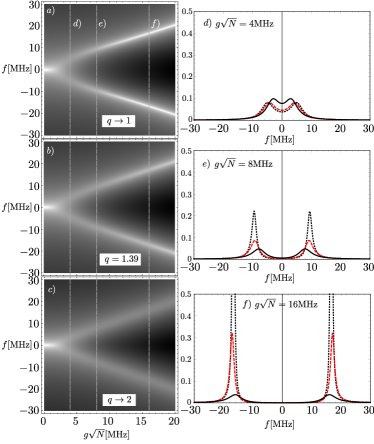
Figure 6: (Color online) We plot $\left|G_{cc}\left(\omega\right)\right|^{2}$ as a function of the collective coupling strength $g\sqrt{N}$ and for three different values of the q-Gaussian parameter $q$ (grayscale figures on the left are plotted on a logarithmic scale). For $g\sqrt{N}=$4,8\,\text{and}\,16\text{\,}\mathrm{MHz}$$, marked by $\left.\text{d}\right)$, $\left.\text{e}\right)$ and $\left.\text{f}\right)$ we show the transmission for all three values of $q$ together. The transmission for the Gaussian coupling density with $q\rightarrow 1$ (dotted black line), for the coupling density of our ensemble with $q=1.39$ (dashed red line) and for the Lorentzian coupling density with $q\rightarrow 2$ (solid black line) are shown on the right. The parameters were chosen to $\gamma_{q}/(2\pi)=$10\text{\,}\mathrm{MHz}$$, $\kappa/(2\pi)=$0.4\text{\,}\mathrm{MHz}$$ and $\gamma_{\text{hom}}/(2\pi)=$1\text{\,}\mathrm{Hz}$$.

To study the behavior of an ensemble following a q-Gaussian distribution with the q-parameter we determined, we show $\left|G_{cc}\left(\omega\right)\right|^{2}$ for $\omega_{c}=\omega_{0}$ as a function of the collective coupling strength $g\sqrt{N}$ in Fig. 6 $\left.\text{b}\right)$. The transmission for an ensemble with Gaussian distribution ($q\rightarrow 1$) is shown in Fig. 6 $\left.\text{a}\right)$ and for a Lorentzian distribution ($q\rightarrow 2$) in Fig. 6 $\left.\text{c}\right)$. The width parameter $a$ is chosen accordingly to ensure that $\gamma_{q}$ is the same for all three cases. In Figs. 6 $\left.\text{d}\right)$-$\left.\text{f}\right)$ the transmission for the three ensemble types is shown for $g\sqrt{N}=$4,8\,\text{and}\,16\text{\,}\mathrm{MHz}$$, respectively. For the ensemble with Lorentzian distribution (solid black line) we see that the width of the Rabi resonances remains constant with increasing collective coupling. For the Gaussian distribution (dotted black line) and the intermediate distribution with $q=1.39$ (dashed red line) we find a decrease in the peak width for increasing collective coupling. In Fig. 7 we plot the real and imaginary part of one of the complex poles of $G^{+}_{cc}\left(\omega\right)$, determining position and width of one of the Rabi peaks. As we focus on the resonant case the spectrum is symmetric. We chose $\gamma_{\text{hom}}=0$, $\kappa/(2\pi)=$0.4\text{\,}\mathrm{MHz}$$, $\gamma_{q}/(2\pi)=$10\text{\,}\mathrm{MHz}$$ and $q=1.39$. This again shows the decreasing width of the Rabi Peaks as $g\sqrt{N}$ increases.

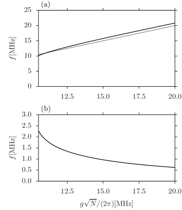
Figure 7: (a) Real part and (b) modulus of the imaginary part of one of the complex poles of $G^{+}_{cc}\left(\omega\right)$ in the regime where $g\sqrt{N}/(2\pi)>\gamma_{q}/(2\pi)=$10\text{\,}\mathrm{M}$\mathrm{Hz}$. The collective coupling strength $g\sqrt{N}$ is shown as dotted line in (a). With increasing $g\sqrt{N}$ the modulus of the imaginary part, proportional to the width of the Rabi peaks, is reduced.

We therefore assume that for our ensemble it is possible to increase the lifetime of the collective states by increasing the collective coupling. This could be achieved by a further decrease of the mode volume or an increase of the NV density in the sample.

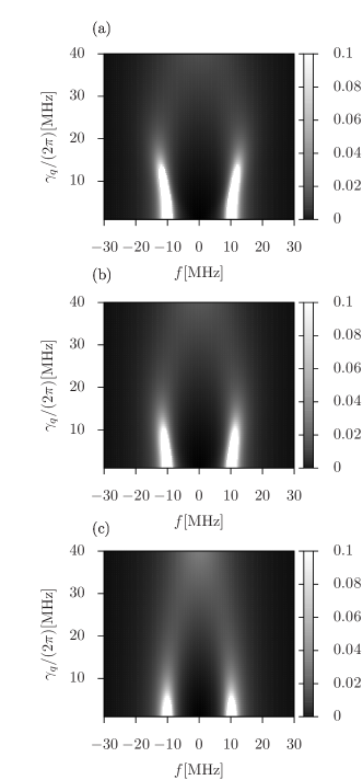
Figure 8: $\left|G_{cc}\left(\omega\right)\right|^{2}$ on resonance as a function of the inhomogeneous width $\gamma_{q}$ for an ensemble with (a) Gaussian coupling density, (b) q-Gaussian $(q=1.39)$ coupling density and (c) Lorentzian coupling density. To keep the transmission visible for large values of $\gamma_{q}$ the range of the color coding is limited to $[0,0.1]$. The parameters were chosen to $g\sqrt{N}/(2\pi)=$10\text{\,}\mathrm{MHz}$$, $\kappa/(2\pi)=$0.4\text{\,}\mathrm{MHz}$$ and $\gamma_{\text{hom}}/(2\pi)=$1\text{\,}\mathrm{Hz}$$.

In Fig. 8 we show the behavior of the transmission with increasing $\gamma_{q}$. For the Lorentzian coupling density the splitting of the resonance peaks is always reduced if $\gamma_{q}>0$. For coupling densities falling off faster than $1/\omega^{2}$, as it is the case in (a) and (b), the splitting of the resonance peaks is even slightly increased for $\gamma_{q}>0$, until the peaks finally merge. Hence a finite but small enough inhomogeneous width might even mimic somewhat higher active spin numbers.

As bottom line we see that common coupling to a cavity mode can suppress dephasing of the polarization, if the effective Rabi frequency is larger than the inhomogeneous width. This could be interpreted as the effect that the exchange of the excitation between the ensemble and the cavity is so fast, that there is no time for decoherence in the ensemble.

IV A transmission line micro-maser with an inhomogeneous NV ensemble

A recent proposal to construct a laser operating on an ultra-narrow atomic clock transition predicted very narrow optical emission above threshold  (Meiser et al., 2009). Similar ideas, employing the collective coupling between a cold atomic ensemble and a microwave cavity, have been proposed to construct stable stripline oscillators in the microwave regime (Henschel et al., 2010).

Here we study the prospects of implementing such an oscillator by coupling a diamond to the CPW resonator. At first sight in view of the MHz scale inhomogeneous broadening, one would expect fast dephasing. However, as we have seen above, for strong enough coupling one observes a continuous rephasing of the polarization inducing a long lived polarization and coherent Rabi oscillations. Thus one could expect narrow microwave emission nevertheless.

Let us consider the case of the cavity mode tuned to resonance with the spin transition $\ket{0}_{\text{I}}\rightarrow\ket{-}_{\text{I}}$, which is partially inverted by an external incoherent pump. Such a pump could in principle be facilitated by optical pumping and it can be consistently modeled by a reversed spontaneous decay. Alternatively one could think of pulsed inversion by tailored microwave pulses or a time switching of the magnetic bias field.

Mathematically such incoherent pumping can be modelled by adding the terms $-\frac{w}{2}\sum_{j=1}^{N}\left(\sigma_{j}^{-}\sigma_{j}^{+}\rho+\rho\sigma_{j}^{-}\sigma_{j}^{+}-2\sigma_{j}^{+}\rho\sigma_{j}^{-}\right)$, where $w$ denotes the pump rate, to the Liouvillian in Eq. 9.

For the explicit calculations, here we use the effective linewidth model, as outlined in Sec. III.2 without any coherent pump. Hence the total phase symmetry of the system is not broken and we assume $\left<a_{c}\right>=\left<a^{\dagger}_{c}\right>=\left<\sigma^{\pm}_{j}\right>=0$. Starting from the master equation in Eq. 8 we derive four coupled equations for $\left<\sigma^{z}_{j}\right>$, $\left<a_{c}^{\dagger}a_{c}\right>$, $\left<a_{c}\sigma_{i}^{+}\right>$ and $\left<\sigma_{i}^{+}\sigma_{j}^{-}\right>$. We used the cumulant expansion $\left<a_{c}^{\dagger}a_{c}\sigma_{i}^{z}\right>=\left<a_{c}^{\dagger}a_{c}\sigma_{i}^{z}\right>_{\text{cum}}+\left<a_{c}^{\dagger}a_{c}\right>\left<\sigma_{i}^{z}\right>$ which takes this simple form because of the total phase invariance. Assuming that the higher order cumulant $\left<a_{c}^{\dagger}a_{c}\sigma_{i}^{z}\right>_{\text{cum}}$ can be neglected, we arrive at a closed set of four equations that can be solved analytically. To study the spectrum of the emitted light we calculate the two-time correlation function $\left<a_{c}^{\dagger}\left(\tau\right)a_{c}\left(0\right)\right>$ via the quantum regression theorem. We switch to a frame rotating with $\omega_{c}$ and define $\Delta=\omega_{-}^{\text{I}}-\omega_{c}$. We obtain

$$\frac{\mathrm{d}}{\mathrm{d}\tau}\begin{pmatrix}\left<a_{c}^{\dagger}\left(\tau\right)a_{c}\left(0\right)\right>\\ \left<\sigma_{i}^{+}\left(\tau\right)a_{c}\left(0\right)\right>\end{pmatrix}=\begin{pmatrix}-\kappa&\mathrm{i}gN\\ -\mathrm{i}g\left<\sigma_{i}^{z}\right>_{\text{st}}&-\left(\frac{w+\gamma_{\text{hom}}}{2}+\gamma_{\text{hom}}\mathrm{bar}{n}\left(T,\omega_{-}^{\text{I}}\right)+\gamma_{p}-\mathrm{i}\Delta\right)\end{pmatrix}\begin{pmatrix}\left<a_{c}^{\dagger}\left(\tau\right)a_{c}\left(0\right)\right>\\ \left<\sigma_{i}^{+}\left(\tau\right)a_{c}\left(0\right)\right>\end{pmatrix}$$ (29)

From Eq. 29 we can calculate the spectrum via Laplace transformation (Meystre and Sargent, 2007). We show the linewidth of the obtained spectrum in the resonant case ($\Delta=0$) for different values of the pump $w$ and the inhomogeneous width $\gamma_{p}$, see Fig. 9.

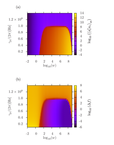
Figure 9: (Color online) In (a) we show the steady state number of photons in the cavity $\left<a_{c}^{\dagger}a_{c}\right>_{\text{st}}$ as a function of the incoherent pump rate $w$ and the inhomogeneous width $\gamma_{p}$. The resulting linewidth $\Delta f$ is shown in (b). For small $\gamma_{p}$ both, $\Delta f$ and $\left<a_{c}^{\dagger}a_{c}\right>_{\text{st}}$ show rapid changes as $w$ becomes larger than $\gamma_{\text{hom}}$. The critical width of the inhomogeneity is given by $\gamma_{p,\text{crit}}=g^{2}N/\kappa$. The parameters were chosen to $N=10^{12}$, $g/(2\pi)=$10\text{\,}\mathrm{Hz}$$, $\kappa/(2\pi)=$1\text{\,}\mathrm{MHz}$$ and $\gamma_{\text{hom}}/(2\pi)=$1\text{\,}\mathrm{Hz}$$.

The minimum linewidth is $\Delta f\approx g^{2}/\kappa$. For small $\gamma_{p}$ the region where we find narrow linewidth emission is characterized by $\gamma_{\text{hom}}<w<2g^{2}N/\kappa$. The critical width of the inhomogeneity is given by $\gamma_{p,\text{crit}}=g^{2}N/\kappa$. Hence once we achieve enough pumping and coupling strength the system could provide for an extremely stable microwave oscillator.

V Conclusions

We showed theoretically and experimentally that an ensemble of spins with an inhomogeneous frequency distribution coupled to a cavity mode can exhibit strong coupling, where the coherent energy exchange between mode and ensemble dominates cavity decay and polarization dephasing. A detailed theoretical modeling connecting probe transmission and frequency distribution allows to extract not only the effective coupling strength and particle number but also the detailed frequency distribution. Interestingly for our dense NV ensemble, the frequency distribution of the spins can be well described as a q-Gaussian with $q=1.39$, showing that the wings of the distribution fall off faster than $1/\omega^{2}$. The temperature dependence of the effective available spin number fits quite well with expectations, except for an unexpected decrease for very low temperature. In summary such an NV ensemble cavity QED system exhibits a prolonged lifetime of the eigenstates of the coupled cavity-ensemble system (Kurucz et al., 2011) and has great potential as quantum interface between superconducting and optical qbits. The long effective $T_{1}$ time could also be the basis of building a compact ultrastable microwave oscillator if the strong coupling overcomes the dephasing from the inhomogeneous broadening.

VI Acknowledgment

K.S. was supported by the DOC-fFORTE doctoral program. R.A. and T.N. were supported by CoQuS, C.K. by FunMat. We acknowledge support by the Austrian Science Fund FWF through the project SFB F40. We thank Klaus Mølmer for his helpful remarks and open discussions.

References

- Phillips et al. (2001) D. Phillips, A. Fleischhauer, A. Mair, R. Walsworth, and M. Lukin, Physical Review Letters 86, 783 (2001).
- Taylor et al. (2008) J. Taylor, P. Cappellaro, L. Childress, L. Jiang, D. Budker, P. Hemmer, A. Yacoby, R. Walsworth, and M. Lukin, Nature Physics 4, 810 (2008).
- Verdú et al. (2009) J. Verdú, H. Zoubi, C. Koller, J. Majer, H. Ritsch, and J. Schmiedmayer, Physical Review Letters 103, 43603 (2009).
- Rabl et al. (2006) P. Rabl, D. DeMille, J. Doyle, M. Lukin, R. Schoelkopf, and P. Zoller, Physical Review Letters 97, 33003 (2006).
- Bushev et al. (2011) P. Bushev, A. Feofanov, H. Rotzinger, I. Protopopov, J. Cole, C. Wilson, G. Fischer, A. Lukashenko, and A. Ustinov, Physical Review B 84, 060501 (2011).
- Kubo et al. (2010) Y. Kubo, F. Ong, P. Bertet, D. Vion, V. Jacques, D. Zheng, A. Dréau, J. Roch, A. Auffeves, F. Jelezko, et al., Physical Review Letters 105, 140502 (2010).
- Amsüss et al. (2011) R. Amsüss, C. Koller, T. Nöbauer, S. Putz, S. Rotter, K. Sandner, S. Schneider, M. Schramböck, G. Steinhauser, H. Ritsch, J. Schmiedmayer, and J. Majer, Physical Review Letters 107, 1 (2011).
- Jelezko and Wrachtrup (2006) F. Jelezko and J. Wrachtrup, physica status solidi (a) 203, 3207 (2006).
- Childress et al. (2006) L. Childress, M. Gurudev Dutt, J. Taylor, A. Zibrov, F. Jelezko, J. Wrachtrup, P. Hemmer, and M. Lukin, Science 314, 281 (2006).
- Acosta et al. (2009) V. Acosta, E. Bauch, M. Ledbetter, C. Santori, K. Fu, P. Barclay, R. Beausoleil, H. Linget, J. Roch, F. Treussart, et al., Physical Review B 80, 115202 (2009).
- Houdré et al. (1996) R. Houdré, R. Stanley, and M. Ilegems, Physical Review A 53, 2711 (1996).
- Diniz et al. (2011) I. Diniz, S. Portolan, R. Ferreira, J. Gérard, P. Bertet, and A. Auffèves, Arxiv preprint arXiv:1101.1842 (2011).
- Kurucz et al. (2011) Z. Kurucz, J. Wesenberg, and K. Mølmer, Physical Review A 83, 053852 (2011).
- Braun et al. (2011) D. Braun, J. Hoffman, and E. Tiesinga, Physical Review A 83, 062305 (2011).
- Carmichael (1993) H. Carmichael, An open systems approach to quantum optics: lectures presented at the Université libre de Bruxelles, October 28 to November 4, 1991, Vol. 18 (Springer, 1993).
- Kubo (1962) R. Kubo, Journal of the Physical Society of Japan 17, 1100 (1962).
- Meiser et al. (2009) D. Meiser, J. Ye, D. Carlson, and M. Holland, Physical Review Letters 102, 163601 (2009).
- Henschel et al. (2010) K. Henschel, J. Majer, J. Schmiedmayer, and H. Ritsch, Physical Review A 82, 033810 (2010).
- Cohen-Tannoudji et al. (1992) C. Cohen-Tannoudji, J. Dupont-Roc, and G. Grynberg, Atom-photon interactions: basic processes and applications (Wiley Online Library, 1992).
- Meystre and Sargent (2007) P. Meystre and M. Sargent, Elements of quantum optics (Springer Verlag, 2007).