Explicit Integration of Extremely-Stiff Reaction Networks: Quasi-Steady-State Methods

Abstract

A preceding paper [1] demonstrated that explicit asymptotic methods generally work much better for extremely stiff reaction networks than has previously been shown in the literature. There we showed that for systems well removed from equilibrium explicit asymptotic methods can rival standard implicit codes in speed and accuracy for solving extremely stiff differential equations. In this paper we continue the investigation of systems well removed from equilibrium by examining quasi-steady-state (QSS) methods as an alternative to asymptotic methods. We show that for systems well removed from equilibrium, QSS methods also can compete with, or even exceed, standard implicit methods in speed, even for extremely stiff networks, and in many cases give somewhat better integration speed than for asymptotic methods. As for asymptotic methods, we will find that QSS methods give correct results, but with non-competitive integration speed as equilibrium is approached. Thus, we shall find that both asymptotic and QSS methods must be supplemented with partial equilibrium methods as equilibrium is approached to remain competitive with implicit methods.

Keywords: ordinary differential equations, reaction networks, stiffness, reactive flows, nucleosynthesis, combustion

1 Introduction

Stiff networks of differential equations rather uniformly have been viewed as requiring special implicit or semi-implicit methods for integration in order to maintain stability while taking reasonably efficient timesteps [2, 3, 4, 5, 6, 7]. Purely explicit methods are not competitive in speed for most applications because they are limited by stability criteria to integration timesteps that are far too short. Various asymptotic and steady-state schemes have been proposed to stabilize explicit methods by removing some of their stiffness (overviews may be found in Refs. [5, 8]). These methods have had some success in moderately stiff systems, but it generally has been concluded that in very stiff systems, such as those encountered in astrophysical thermonuclear networks, asymptotic and steady-state schemes do not work [5, 8].

In a preceding paper on asymptotic methods [1], the present paper on quasi-steady-state (QSS) methods, and a following paper on partial equilibrium methods [9], we challenge these conclusions and present strong evidence that algebraically-stabilized explicit integration may in fact not only compete with, but in some cases may have the potential to outperform traditional implicit methods, even for the stiffest networks. In this paper we deal specifically with the QSS method and show that, for systems well removed from equilibrium, the QSS approximation can give highly-competitive integration of extremely-stiff systems.

2 Quasi-Steady-State Approximations

Let us begin by introducing the quasi-steady-state approximation. We wish to solve $N$ coupled ordinary differential equations

$$\frac{dy_{i}}{dt} = F_{i}(y,t)=\sum_{j}F_{ij}(t)$$ (1)

$$\equiv F^{+}_{i}(t)-F^{-}_{i}(t)=F^{+}_{i}(t)-k_{i}(t)y_{i}(t)$$

where $y_{i}(i=1\dots N)$ describes the dependent (abundance) variables, $t$ is the independent variable (time in our examples), $F_{ij}$ denotes the flux between species $i$ and $j$, the sum for each variable $i$ is over all variables $j$ coupled to $i$ by a non-zero flux $F_{ij}$, and the flux has been decomposed into a component $F^{+}_{i}$ increasing the abundance of $y_{i}$ and a component $F^{-}_{i}$ depleting it. For an $N$-species network there will be $N$ such equations in the populations $y_{i}$, and they generally will be coupled to each other because of the dependence of the fluxes on the different $y_{j}$.

If one attempts to integrate these equations numerically by ordinary forward difference, severe stability problems will be encountered for networks in which the various rate parameters appearing in the terms on the right side of Eq. (1) range over many orders of magnitude in size. This is the problem of stiffness. The traditional solution is to invoke implicit methods, which are stable even in the face of extremely stiff equations. An alternative explicit algebraic solution to the coupled differential equations uses the Quasi-Steady-State (QSS) approximations developed by Mott and collaborators [8, 10], which was partially motivated by earlier work in Refs. [11, 12, 13]. We follow Mott et al [8, 10] by first noting that Eq. (1) in the form

$$\frac{dy}{dt}=F^{+}(t)-k(t)y(t)\qquad y(0)\equiv y_{0}$$ (2)

(where we have suppressed indices for notational convenience) has the analytical solution

$$y(t)=y_{0}e^{-kt}+\frac{F^{+}}{k}(1-e^{-kt}),$$ (3)

for constant $k$ and $F^{+}$. In the QSS method this equation then serves as the basis of a predictor–corrector scheme in which a prediction is made using initial values and a corrector is then applied that uses a combination of initial values and values computed using the predictor solution. Defining a parameter $\alpha(r)$ by

$$\alpha(r)=\frac{160r^{3}+60r^{2}+11r+1}{360r^{3}+60r^{2}+12r+1},$$ (4)

where $r\equiv 1/k\Delta t$ with $\Delta t$ the integration timestep, we adopt a predictor $y^{\mbox{\scriptsize p}}$ and corresponding corrector $y^{\mbox{\scriptsize c}}$ proposed originally by Mott et al [8, 10],

$$y^{\mbox{\scriptsize p}}=y^{0}+\frac{\Delta t(F_{0}^{+}-F_{0}^{-})}{1+\alpha^{0}k^{0}\Delta t}\qquad y^{\mbox{\scriptsize c}}=y^{0}+\frac{\tilde{F}^{+}-\bar{k}y^{0}}{1+\bar{\alpha}\bar{k}\Delta t},$$ (5)

where $\alpha^{0}$ is evaluated from Eq. (4) with $r=1/k^{0}\Delta t$, an average rate parameter is defined by $\bar{k}=\mbox{$\small\frac{1}{2}$}(k^{0}+k^{\mbox{\scriptsize p}})$, $\bar{\alpha}$ is specified by Eq. (4) with $r=1/\bar{k}\Delta t$, and

$$\tilde{F}^{+}=\bar{\alpha}F_{\scriptstyle\rm p}^{+}+(1-\bar{\alpha})F_{0}^{+}.$$

If desired, the corrector can be iterated by using $y^{\mbox{\scriptsize c}}$ from one iteration step as the $y^{\mbox{\scriptsize p}}$ for the next iteration step. We implement an explicit QSS algorithm based on the predictor–corrector pair (5) in a manner analogous to that described in the preceding paper for the asymptotic method [1], except that for the QSS algorithm we treat all equations by the QSS approximation, rather than dividing them into a set treated by explicit forward difference and a set treated in asymptotic approximation, as we did in Ref. [1].

3 Adaptive Timestepping

To integrate the equations (1) using the predictor–corrector (5), we employ a simple timestepping algorithm analogous to that already described in more detail in the preceding asymptotic paper [1]:

1. At the beginning of a new timestep, compute a trial timestep based on limiting the change in population that would result from that timestep to a specified tolerance. Choose the minimum of this trial timestep and the timestep that was taken in the previous integration timestep as the timestep, and update all populations by the quasi-steady-state algorithm described above.

2. Check the results for conservation of particle number within a specified tolerance range. If the condition is not satisfied, increase or decrease the timestep as appropriate by a small factor and repeat the calculation with the original fluxes. Accept this result for the populations and carry the new timestep over as a starting point for the next timestep.

This timestepper is not particularly sophisticated but we have found it to be stable and accurate for a variety of astrophysical thermonuclear networks that we have tested.

4 Equilibrium and Stiffness

As we have discussed in more detail in Refs. [1, 9], there are two forms of equilibrium that concern us in explicit integration of stiff reaction networks. These may be displayed clearly if we decompose $F^{+}_{i}$ and $F^{-}_{i}$ for a species $i$ in Eq. (1) into a set of terms depending on the other populations in the network (labeled by the index $j$),

$$\frac{dy_{i}}{dt} = F^{+}_{i}-F^{-}_{i}$$ (6)

$$= (f_{1}^{+}+f_{2}^{+}+\ldots)_{i}-(f_{1}^{-}+f_{2}^{-}+\ldots)_{i}$$

$$= (f_{1}^{+}-f_{1}^{-})_{i}+(f_{2}^{+}-f_{2}^{-})_{i}+\ldots=\sum_{j}(f^{+}_{j}-f^{-}_{j})_{i},$$

We shall refer to macroscopic equilibration if $F^{+}_{i}-F^{-}_{i}$ approaches a constant. This is the basis for the asymptotic approximations discussed in Ref. [1] and the quasi-steady-state approximation to be discussed in this paper. However, at a more microscopic level, groups of individual terms on the right side of Eq. (6) may come approximately into equilibrium (so that the sum of their fluxes is approximately zero), even if the macroscopic conditions for equilibration are not satisfied. This corresponds to equilibration for individual forward–reverse reaction pairs such as $A+B+\ldots\rightleftharpoons C+D+\ldots$ . This process, which may occur even if the conditions for macroscopic equilibration are not satisfied, we shall term microscopic equilibration. These definitions then permit us to identify three distinct categories of stiffness that may occur in a reaction network [1]:

1. Small populations can become negative if the explicit timestep is too large, with the propagation of this anomalous negative population leading to destabilizing terms that grow exponentially.

2. Macroscopic equilibration, where taking the difference $F^{+}-F^{-}$ leads to large errors if the timestep is too large.

3. Microscopic equilibration, where taking the net flux in specific forward-reverse reaction pairs $(f^{+}_{i}-f^{-}_{i})$ leads to large errors if the timestep is too large.

These distinctions are crucial for our goal of integrating stiff equations explicitly by identifying sources of stiffness in the network and removing them by algebraic means because the QSS method and asymptotic methods remove only the first two kinds of stiffness. Removal of the third kind of stiffness will require the partial equilibrium methods that will be discussed in the third paper in this series [9]. Thus, it will be important for our discussion to have a quantitative measure of microscopic equilibration. We shall describe this in detail in Ref. [9] for thermonuclear networks, and the basics have been worked out by Mott [8], so we just quote without proof the results that will be relevant for the present discussion.

We assume that the amount of microscopic equilibration in a network is measured by the fraction of forward–reverse reaction pairs $A+B+\ldots\rightleftharpoons C+D+\ldots$ that are judged to be in equilibrium (with each reaction pair considered separately). The variation of the populations $y_{i}$ with time during a numerical integration timestep may be approximated for each reaction pair by a differential equation

$$\frac{dy_{i}}{dt}=ay_{i}^{2}+by_{i}+c,$$ (7)

where the parameters $a$, $b$, and $c$ are known functions of the current rate parameters and the abundances at the beginning of the timestep. This equation may be solved for the equilibrium abundance $\bar{y}_{i}$ of each species, giving

$$\bar{y}_{i}\equiv y^{{\rm\scriptstyle eq}}_{i}=-\frac{1}{2a}(b+\sqrt{-q}).$$ (8)

where $q\equiv 4ac-b^{2}$ and the single timescale $\tau=q^{-1/2}$ governs the approach to equilibrium. We may then estimate whether a given reaction is near equilibrium at time $t$ by requiring

$$\frac{|y_{i}(t)-\bar{y}_{i}|}{\bar{y}_{i}}<\epsilon_{i}$$ (9)

for each species $i$ involved in the reaction, where $y_{i}(t)$ is the actual abundance, $\bar{y}_{i}$ is the equilibrium abundance (8), and $\epsilon_{i}$ is a tolerance, typically of order $10^{-2}$. The remainder of this paper will emphasize methods based on quasi-steady-state approximations to stabilize explicit integration for networks that are at most weakly equilibrated by the above criteria, with the corresponding stabilization of networks near equilibrium to be discussed in [9].

5 Explicit and Implicit Integration Speeds for a Timestep

In examples to be shown below we shall be comparing explicit and implicit methods using codes that are at very different stages of development and optimization. Thus they cannot simply be compared head to head. Implicit methods spend increasing amounts of integration time inverting matrices as networks become larger. Thus, explicit methods—which require no matrix inversions—can generally compute each timestep faster. Let us assume roughly that the speedup factor for explicit versus implicit methods for integrating a timestep is $F=1/(1-f)$, where $f$ is the fraction of computing time spent by the implicit algorithm in matrix operations. Using data obtained by Feger [14, 15] with the implicit, backward-Euler code Xnet [16] employing both dense and sparse matrix solvers, we adopt for our discussion the factors $F$ listed in Table 1.

Table 1: Explicit-method speedup factors [15]

• Network	Isotopes	Speedup $F$
  CNO (main)	8	$\sim 1.5$
  Alpha	16	3
  CNO extended	18	3
  Nova	134	7
  150-isotope	150	7.5
  365-isotope	365	$\sim 20$

We will then make a simple estimate of the relative speed of explicit versus implicit algorithms by multiplying the factor $F$ by the ratio of integration timesteps for implicit and explicit integrations for a given problem. This probably underestimates the relative speed of an optimized explicit versus optimized implicit code for reasons discussed in Ref. [17], but it will allow us to place a lower bound on how fast the explicit calculation can be.

6 Comparison of QSS Methods with Asymptotic and Implicit Methods

In earlier applications of asymptotic and steady-state methods in chemical reaction networks, evidence was presented that Quasi-Steady-State (QSS) approximations gave more accurate, stable, and faster solutions than asymptotic approximations [8, 10], but that both approximations failed when applied to the extremely stiff systems characteristic of astrophysical thermonuclear networks [5, 8]. In a preceding paper we have investigated the use of explicit asymptotic approximations for extremely stiff astrophysical networks and concluded that the asymptotic approximation in fact works quite well for even the stiffest networks, provided that they are not too close to equilibrium [1]. We now wish to revisit the utility of QSS methods for extremely stiff networks, comparing them with results from both asymptotic and implicit calculations for some representative extremely stiff astrophysical networks of varying sizes. In the general case, we shall find that both asymptotic and QSS methods are capable of solving extremely stiff networks stably and accurately, but that QSS approximations often allow somewhat larger timesteps than the corresponding asymptotic approximation calculation. We shall find that these timesteps for both QSS and asymptotic approximations are often quite competitive with those of a standard implicit code for systems that are not near microscopic equilibrium.

6.1 Appropriate Astrophysical Variables

For the astrophysical examples given in the remainder of this paper, the generic population variables $y_{i}$ (assumed to be proportional to the number density for the species $i$) will be replaced with the mass fractions $X_{i}$. These satisfy

$$X_{i}=\frac{n_{i}A_{i}}{\rho N_{\mbox{\scriptsize A}}}\qquad\sum_{i}X_{i}=1,$$ (10)

where $N_{\mbox{\scriptsize A}}$ is Avogadro’s number, $\rho$ is the total mass density, $A_{i}$ is the atomic mass number, and $n_{i}$ is the number density for the species $i$.

6.2 CNO Cycle and the pp-Chains

Fig. 1 illustrates a comparison of QSS, asymptotic, and implicit methods for the main branch of the astrophysical CNO cycle,

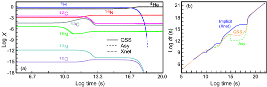
Figure 1: Comparison of asymptotic, quasi-steady-state, and implicit approximations for the main branch of the CNO cycle at a constant temperature of 20 million K ($T_{9}=0.020$) and constant density $\rho=20\mbox{\ g\,cm}^{-3}$, with initial abundances of solar composition. This network corresponds to 8 isotopes and 18 reaction couplings, with reaction rates taken from the REACLIB library [18]. (a) Isotopic mass fractions. Solid curves are implicit (Xnet [16]), dashed are QSS and asymptotic. (b) Integration timesteps. The calculation shown used three iterations for the QSS method, which provided marginal improvement over a single iteration.

which is illustrated in Fig. 2.

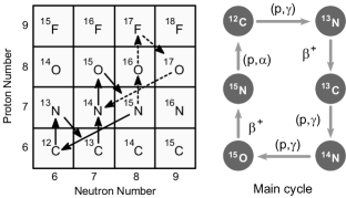
Figure 2: The CNO cycle. The main branch of the cycle is illustrated with solid arrows and a side branch is illustrated with dashed arrows. The main branch of the CNO cycle is illustrated schematically with more detail on the right side.

The calculated mass fractions are almost identical for the three approaches. The timestepping for the QSS and asymptotic integrations is also very similar, except for a small region approaching hydrogen depletion ($\log t\sim 17$) where the QSS method is able to take timesteps 1-2 orders of magnitude larger than the asymptotic method. This translates into an overall improvement of roughly a factor of two in time to complete the calculation. The timestepping for the implicit method is seen to be very similar to that of the two explicit methods except for the range $\log t=15$ to $\log t=18$, where the implicit method averages 10–100 times larger timesteps than the QSS method. The fastest stable timestep for a purely explicit method in this calculation is of order 100 seconds and therefore is far off the bottom of the scale in Fig. 1. We note that at the end of the calculation the QSS and asymptotic timesteps are about $10^{20}$ times larger than would be stable for a purely explicit calculation.

Although this larger timestepping for the implicit method is confined to a small region in Fig. 1, this is quite significant for the overall integration time (a fact partially obscured by the log–log plot). The two explicit methods spend the bulk (97% for the asymptotic calculation, for example) of their total integration times in the region from $\log t=15$ to $\log t=18$, where the implicit integration is taking timesteps 10–100 times larger than the explicit methods. This translates into 292 total integration steps for the implicit code, 15,484 for QSS, and 210,398 for the asymptotic calculation. The explicit methods, once optimized, may be expected to compute these timesteps faster, but for a network this small that advantage will likely be only a factor of two or so (Table 1). Thus the QSS method needs at least another factor of 25 in speed for the calculation of Fig. 1 to compete with the fastest implicit integration of the CNO cycle. That is not very important practically for a single integration of this simple network, since any of the three methods can integrate it to hydrogen depletion in a fraction of a second on a modern processor, but if the network were integrated many times the difference would become significant.

In Fig. 3 we compare QSS, asymptotic, and fully implicit calculations for an extended CNO network

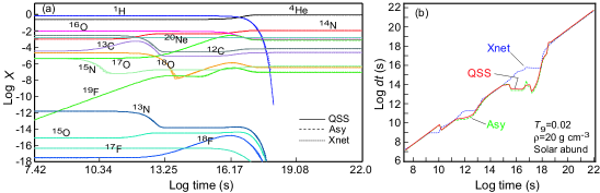
Figure 3: Comparison of implicit (Xnet), quasi-steady-state, and asymptotic approximations for an extended CNO cycle at a constant temperature of $T_{9}=0.020$ and constant density $\rho=20\mbox{\ g\,cm}^{-3}$, with initial abundances of solar composition. This network corresponds to 18 isotopes and 131 reaction couplings, with reaction rates taken from the REACLIB library [18]. (a) Isotopic mass fractions. (b) Integration timesteps. The calculation shown used 1 iteration for the QSS method.

(corresponding to the full network shown on the left side of Fig. 2 plus several additional isotopes). In this case we see that all three methods give essentially the same mass fractions and similar timestepping, except for a short period near $\log t\sim 15-18$ where the implicit calculation takes timesteps as much as 100 times larger than the other methods. Note that in this example there is almost no difference between the QSS and asymptotic timestepping, unlike the case in Fig. 1 where the QSS calculation is faster. Once again, the log–log scale somewhat obscures that the explicit methods need another factor of $\sim$15 in speed to be as fast as the implicit calculation (the implicit code took 348 total steps, the QSS code took 10,101 steps, and the asymptotic code took 13,095 steps for this case), but all three methods can compute the network to hydrogen depletion in less than a second of processor time. As for Fig. 1, the fastest stable timestep for a purely explicit method in this calculation is of order 100 seconds and therefore is off the bottom of the scale in Fig. 3. At the end of the calculation the QSS and asymptotic timesteps are about $10^{19}$ times larger than would be stable for a purely explicit calculation.

We speculate that the reason the QSS and asymptotic timesteps lag behind the implicit method timesteps only for the range $\log t\sim 15-18$ is that this is roughly the time period when the CNO cycle is running in steady state (approximately constant abundances for the carbon–nitrogen–oxygen isotopes, as hydrogen is being converted to helium at a nearly constant rate), up until the hydrogen begins to be significantly depleted; see Fig. 1(a). In that period the CNO cycle running in steady state establishes a new timescale in the system, which is the time characteristic of restoring the cycle equilibrium if it were disturbed. From Fig. 1(a) we may estimate that this timescale is approximately $\tau\sim 10^{13}-10^{14}$ s, since this was the time to establish steady state initially. Neither the asymptotic nor QSS approximations remove the specialized stiffness associated with this cycling timescale completely (nor would the partial equilibrium approximation as we have formulated it, since the cycle does not have reversible reactions). Thus the explicit timestep stops growing around $dt\sim 10^{13}-10^{14}$ s because substantially larger explicit timesteps would not be able to resolve and respond to fluctuations in the CNO equilibrium. This remains true until the onset of hydrogen depletion removes this timescale and the explicit method is again able to increase its timesteps rapidly. This suggests that a modification of the explicit methods to replace the cycle with an analytical approximation when it is running near steady state should permit the explicit methods to increase their timesteps competitively in the time period $\log t\sim 15-18$.

In the preceding CNO-cycle calculations the implicit method is superior, performing the integration more than an order of magnitude faster than the explicit methods. However, the remarkable result is not that the implicit algorithm is faster. Rather, it is that the QSS method has made up almost 19 of the 20 orders of magnitude difference between the integration speed of a purely explicit method relative to the implicit method, and that the remaining order of magnitude is likely because of a highly-specialized stiffness associated with cycling that has not yet been dealt with in the explicit networks. This interpretation is bolstered by applying the QSS method to the astrophysical pp-chains, which are comparable in stiffness to the CNO cycle but do not exhibit cycling. Figure 4

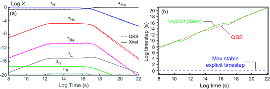
Figure 4: Integration of the pp-chains at constant temperature $T_{9}=0.016$ (where $T_{9}$ denotes temperature in units of $10^{9}$ K) and constant density $160\mbox{\ g\,cm}^{-3}$, assuming solar initial abundances. Reaction rates were taken from the REACLIB library [18]. (a) Mass fractions for the asymptotic method, the QSS method, and for the standard implicit code Xnet [16]. (b) Integration timesteps.

displays integration of the pp-chains at a constant temperature and density characteristic of the core in the present Sun using the QSS method and the implicit backward-Euler code Xnet [16]. In this example we see that the QSS method has made up essentially all of the more than 20 orders of magnitude difference between implicit and purely explicit timestepping. This gives integration speeds about the same as for the implicit method: the implicit code required only 176 integration steps versus 286 for the QSS method, but from Table 1 each timestep for the 7-isotope pp-chain network can probably be calculated $\sim$1.5 times faster using the explicit code.

6.3 Type Ia Supernova Detonation Waves

In Fig. 5

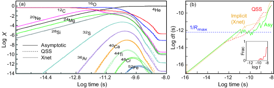
Figure 5: Comparison of asymptotic and quasi-steady-state approximations for an alpha network at a constant temperature of $T_{9}=10$ and constant density $\rho=5\times 10^{7}\mbox{\ g\,cm}^{-3}$, with initial equal mass fractions of ¹²C and ¹⁶O, and reaction rates specified by REACLIB [18]. The network contained 16 isotopes with 46 reaction couplings. Also shown are results from the implicit code Xnet [16]. (a) Isotopic mass fractions. (b) Integration timesteps. Solid curves are asymptotic, dashed curves are QSS, and dotted curves are implicit; the dotted blue curve estimates the maximum stable purely explicit timestep. The inset to (b) shows the fraction of reactions equilibrated as a function of time. The calculation shown used one iteration for the QSS method; additional iterations did not lead to substantial improvement.

we compare asymptotic and QSS calculations for an alpha-particle network at a constant temperature of $T_{9}=10$ and constant density $\rho=5\times 10^{7}\mbox{\ g\,cm}^{-3}$, which represents conditions that might be found for a strong detonation wave in a Type Ia supernova simulation. We see that the mass fractions computed in the two cases are essentially the same, except for some small differences in the weaker populations near $\log t\sim-9$. At earlier times the asymptotic method gives somewhat larger timesteps but at intermediate times corresponding to maximal burning the QSS timesteps are as much as an order of magnitude larger. The QSS and asymptotic integration times are also seen to be rather competitive with those of the implicit calculation. The total calculation required 1464 asymptotic timesteps, 714 QSS timesteps, and 329 implicit timesteps. Since an explicit timestep can be computed about 3 times faster by the explicit methods relative to the implicit method for this 16-isotope network (Table 1), equivalently-optimized versions of all three methods would be rather similar in speed.

Consulting the inset to Fig. 5(b), we see that almost no reactions become microscopically equilibrated until very late in the calculation, which explains the competitive explicit QSS and asymptotic timesteps over most of the integration range. Although the amount of partial equilibrium is small until late in the preceding calculation, this still has a significant negative impact on the QSS and asymptotic timesteps. In Ref. [9] we shall implement a partial equilibrium formalism to deal with this. If those methods are applied to the present problem, the required number of integration steps is reduced from 714 to 313 for the QSS method and from 1464 to 322 for the asymptotic method. Thus, with partial equilibrium accounted for the calculation of Fig. 5 would become several times faster for both QSS and asymptotic methods relative to the implicit calculation, by virtue of the speedup factor of about 3 for the explicit method from Table 1.

The QSS method can be iterated to improve the solution [10]. The calculation shown in Fig. 1 used three QSS iterations, but a single iteration gave results almost as good. The calculation shown in Fig. 5 used a single iteration and was not significantly improved by additional iterations. In our tests on very stiff thermonuclear networks, we have found that iterating the QSS solution does not generally give significantly better results than a single-iteration calculation, but can improve the speed corresponding to a given precision in some cases by factors of two.

In Fig. 6

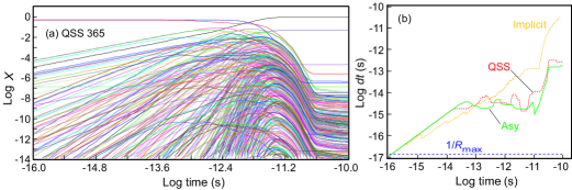
Figure 6: A 365-isotope network integrated at constant temperature $T_{9}=10$ and constant density $\rho=5\times 10^{7}\mbox{\ g\,cm}^{-3}$, for an initial concentration of half ¹²C and half ¹⁶O by mass fraction. The network contained 365 isotopes and 4325 reaction couplings, with the reaction rates supplied by REACLIB [18].(a) Isotopic mass fractions for the quasi-steady-state (QSS) method. (b) Integration timesteps for the asymptotic method (solid green curve), the QSS method (dashed red curve), and the implicit code Xnet [16] (dotted orange curve). The maximum stable timestep for a normal explicit calculation (dashed blue curve) was estimated as the inverse of the fastest rate in the network.

we display mass fractions for the QSS method and compare timestepping for the QSS, asymptotic, and explicit methods for the same conditions as in Fig. 5, but for a 365-isotope network. Since there are so many mass-fraction curves in Fig. 6(a), we do not attempt to compare them directly with an asymptotic or implicit calculation. However, in Ref. [1] we established the equivalence of mass fractions calculated by standard implicit and asymptotic approximations, and in Fig. 7(a)

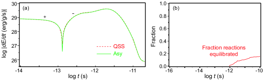
Figure 7: (a) Comparison of differential energy production calculated by QSS (dotted red curve) and asymptotic approximations [1] (solid green curve) for the 365-isotope network of Fig. 6. The energy production changes sign near $\log t=-13$, so we plot the log of the absolute value of $dE/dt$ and indicate its sign on the curve. (b) Fraction of reactions microscopically equilibrated in the QSS calculation.

we compare the differential energy production (a strong proxy for evolution of the isotopic number densities) for the network in Fig. 6 calculated by QSS and asymptotic methods. The curves are in almost perfect agreement, and the integrated energy release corresponding to the simulation of Fig. 6 differed by less than 0.2% between QSS and asymptotic calculations.

For this example the QSS calculation used two iterations of the predictor–corrector algorithm (5), which permitted almost a factor of two larger timestep size than for one iteration. Computing the rates is the most time-consuming operation in an explicit timestep. Since a predictor–corrector iteration recomputes the fluxes by multiplying the rates by the new populations from the predictor step but does not recompute the rates, it does not cost much. In this case, once the rates have been calculated at the current temperature and density, each iteration increases the time to compute the timestep by only a few percent.

The methods all take similar timesteps until $\log t\sim-12$, after which the QSS calculation takes somewhat larger timesteps than the asymptotic method, while the implicit calculation takes timesteps that average about 10 times larger than the QSS method. As a result, for the entire calculation the implicit code required 444 integration steps, the QSS code required 4398 steps, and the asymptotic code required 9739 steps. The timestep advantage of the implicit code over the QSS code by about a factor of 10 will be approximately canceled by the $\sim 20$ times faster computation of each timestep by the explicit code for a 365-isotope network (see Table 1). Thus, for the case in Fig. 6 we expect that for optimized codes the QSS and implicit methods would have similar speeds, and the asymptotic method would be about a factor of two slower.

In Fig. 7(b) we plot the fraction of reactions in the network that become microscopically equilibrated. The reason that the implicit code is able to take larger timesteps than the explicit codes for $\log t>-12$ in the 365-isotope case now becomes clear: that is exactly where partial equilibrium begins to play a role. Because the fraction of partially-equilibrated reactions reaches only $\sim$15% in this calculation, the explicit methods are still able to compete favorably, but as we have already seen for the alpha network of Fig. 5, and as we shall see further later in this paper and in Ref. [9], even a small partial-equilibrium fraction can have a large negative influence on the explicit integration timestep. The impact on the total integration time for the present examples will be amplified because the QSS calculation in Fig. 6 expends more than 90% of its integration steps for times where partial equilibrium is significant (while in the alpha network of Fig. 5 the corresponding fraction is about 75%). Thus, we may expect that a proper treatment of partial equilibrium in this case should lead to an explicit QSS or asymptotic timestep that is much larger, implying a substantial speed advantage for each of the two explicit methods versus the implicit method, once proper account has been taken of partial equilibrium.

6.4 Tidal Supernova Simulation

A comparison of asymptotic and QSS mass fractions and timesteps is shown in Fig. 8

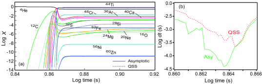
Figure 8: Comparison of asymptotic and quasi-steady-state approximation calculations for an alpha network calculation using the hydrodynamical profile shown in Fig. 9. (a) Mass fractions (solid lines asymptotic, dashed lines QSS; they are almost indistinguishable). (b) Integration timesteps for asymptotic (solid) and QSS (dashed) in the strong burning region. The QSS calculation shown used three iterations but one or two iterations gave similar results.

for an alpha network with a hydrodynamical profile characteristic of a supernova induced by tidal interactions in a white dwarf (illustrated in Fig. 9).

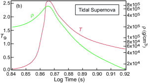
Figure 9: Hydrodynamical profiles for temperature and density under tidal supernova conditions [19].

We see that in the critical strong-burning region the QSS approximation is able to take timesteps that are about an order of magnitude faster than the asymptotic method. (Outside this region the timesteps are similar for the two methods.) The timestepping over the entire integration range is compared for QSS, an asymptotic calculation, and the implicit code Xnet in Fig. 10(a).

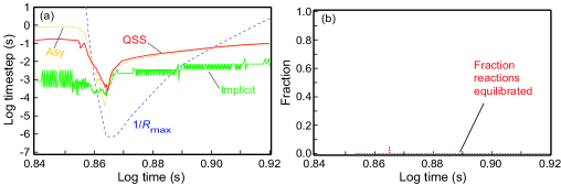
Figure 10: (a) QSS integration timesteps (solid red), Asymptotic integration timesteps (dotted orange), integration steps for the implicit code Xnet [16] (solid green), and maximum stable purely-explicit step (dashed blue), for the calculation in Fig. 8. (b) Fraction of isotopes that become asymptotic and fraction of reactions equilibrated in the network.

The QSS timestepping (242 total integration steps) is somewhat better than for the asymptotic method (480 steps) and considerably better than for the implicit code (2136 steps). For an alpha network an optimized explicit code can compute timesteps about three times as fast as an implicit code (Table 1), so we may estimate that the QSS code is capable of calculating this network some 15 times faster, and the asymptotic code perhaps 10 times faster, than the implicit code. Results almost as good as those presented above for networks under tidal supernova conditions using the QSS method have been found in Refs. [14, 15] using the explicit asymptotic method. Although a different set of reaction network rates was used in these references, the explicit asymptotic method was found to be highly competitive with standard implicit methods for the tidal supernova problem.

The good QSS and asymptotic timestepping for this case is primarily because essentially no reactions in the network come into equilibrium, as illustrated in Fig. 10(b). Note in this connection that the flat mass fraction curves at late times in Fig. 8(a) are not a result of equilibrium, but rather of reaction freezeout caused by the temperature and density dropping quickly at late times as the system expands (see Fig. 9). It is this rapid decrease of all thermal reaction rates to zero at later times that prevents microscopic equilibration from playing a significant role for this case.

The dashed blue curve in Fig. 10(a) represents the estimated fastest stable purely-explicit timestep. By comparing this curve with the QSS and asymptotic timestep curves we see that, unlike most of the cases we are investigating, this system is only moderately stiff. The maximum difference between the actual timestep and the maximum stable purely-explicit timestep is about 4 orders of magnitude. Furthermore, for $\log t<0.86$ and $\log t>0.9$ the maximum stable purely-explicit timestep is larger than the actual timestep; thus in these regions the stiffness instability plays no role in setting the explicit QSS or explicit asymptotic timestep. This might suggest that it is the relatively moderate stiffness of this problem compared with most in astrophysics that makes the QSS and asymptotic methods particularly efficient for this case. However, comparison with a number of other cases (see for example, the nova calculation in §6.5) indicates that this is not correct: it is not the amount of stiffness (as inferred from differences in ranges of timescales in the problem) but rather the nature of the stiffness that is crucial. The QSS and asymptotic methods are capable of removing many orders of magnitude of stiffness caused by macroscopic equilibration (for example, see Fig. 12(a) below), but are poor at removing stiffness caused by microscopic equilibration.

6.5 Nova Explosions

Let us turn now to an example involving a large and extremely stiff network. In Fig. 11(a)

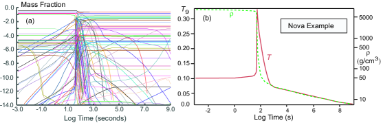
Figure 11: (a) Mass fractions for a network under nova conditions, corresponding to the hydrodynamical profile shown in (b). The calculation used the QSS method and a network containing 134 isotopes coupled by 1531 reactions, with rates taken from the REACLIB library [18] and initial abundances enriched in heavy elements [20].

we illustrate a calculation using the explicit QSS algorithm with a hydrodynamical profile displayed in Fig. 11(b) that is characteristic of a nova outburst. Given the large number of mass-fraction curves, we do not attempt to compare them directly with an asymptotic or implicit calculation, but we note that the total integrated energy release corresponding to the simulation of Fig. 11 was within 1% of that found for the same network using the explicit asymptotic approximation in Ref. [1]. The integration timesteps for the calculation in Fig. 11(a) are displayed in Fig. 12(a).

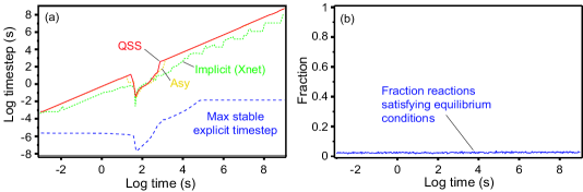
Figure 12: (a) Timesteps for integration of Fig. 11. The solid red curve is from the QSS calculation. The dotted orange curve is from an explicit asymptotic calculation [1]. The dotted green curve is from an implicit integration using the backward-Euler code Xnet [16]. The dashed blue curve estimates the largest stable fully explicit timestep as the inverse of the fastest rate in the system. (b) Fraction of reactions that reach partial equilibrium in the QSS calculation.

Once burning commences, the QSS solver (solid red curve in Fig. 12(a)) takes timesteps that are from $10^{6}$ to $10^{10}$ times larger than would be stable for a normal explicit integration.

The explicit QSS timesteps illustrated in Fig. 12(a) are somewhat larger than those of our asymptotic solver (dotted orange curve), and comparable to or greater than those for a typical implicit code over the whole integration range, as may be seen by comparing with the implicit (backward Euler) calculation timestepping curve shown in dotted green. In this calculation the implicit method required 1332 integration steps, the explicit asymptotic calculation required 935 steps, and the QSS method required 777 steps. Given that for a network with 134 isotopes the explicit codes should be able to calculate an integration timestep about 7 times faster than an implicit code because they avoid the manipulation of large matrices (Table 1), these results suggest that the explicit QSS code is capable of calculating the nova network more than 10 times faster and the explicit asymptotic code more than 5 times faster than a state-of-the-art implicit code.

This impressive integration speed for both the QSS and asymptotic methods applied to a large, extremely stiff network is possible because few reactions reach microscopic equilibrium during the simulation, as illustrated in Fig. 12(b). Thus the entire nova simulation, just as for the tidal supernova simulation and the Type Ia supernova detonation wave simulation until very late in the calculation, lies within a domain where we expect both the QSS and asymptotic explicit methods to be highly effective in removing stiffness from the network. In Refs. [14, 15] the explicit asymptotic method was applied to a nova simulation. Although this calculation differed from the present one in using asymptotic methods, a different nova hydrodynamical profile, and a different reaction library, results rather similar to those presented above were obtained. We conclude that the explicit QSS and asymptotic methods may intrinsically be considerably faster than a state-of-the art implicit code for simulations of nova outbursts.

7 Non-Competitive QSS Timesteps in the Approach to Equilibrium

Except for late in the calculation for the supernova detonation wave in §6.3, the examples shown to this point have involved networks in which few reactions have become microscopically equilibrated by the criteria of §4. For such cases we have seen that the integration speed for QSS and asymptotic explicit methods is often comparable to, and in some cases exceeds, that for current implicit codes. Let us now turn to a representative example where this is no longer true. The calculation in Fig. 13

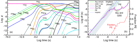
Figure 13: Comparison of asymptotic and quasi-steady-state approximations for an alpha network with constant temperature $T_{9}=5$ and constant density of $10^{8}\mbox{\ g\,cm}^{-3}$, using REACLIB rates [18] and initial equal mass fractions of ¹²C and ¹⁶O. (a) Isotopic mass fractions. (b) Integration timesteps (left axis) and fraction of reaction in partial equilibrium (right axis). The gray shaded area represents roughly the region that the explicit timestep profile must lie in to have a chance to compete with implicit methods. The different asymptotic methods are labeled Asy and are described in Ref. [1]. The implicit calculation was made with Xnet [16] and the dashed green line (PE) represents the timestepping for a partial equilibrium calculation that will be discussed in a later publication [9]. The QSS calculation was run with a single iteration.

compares QSS and several different asymptotic approximations with an implicit calculation for an alpha network at a constant temperature and density characteristic of a Type Ia supernova explosion. We may draw two important conclusions from these results.

1. Although there are some differences among the QSS and various asymptotic methods, we see that they all give essentially the same results, with timestepping that is rather similar, though timestepping differences of up to factors of 5-10 may be found in localized time regions. All of the QSS and asymptotic cases shown have integrated final energies that lie within 1% of each other and their total integration times are all within 25% of each other.

2. The QSS method and the various asymptotic methods all give timesteps that potentially are competitive with implicit methods at early times, but they fall far behind at late times.

The reason for the non-competitive nature of the asymptotic and QSS timestepping at late times in this calculation can be seen clearly from the solid red curve on the right of Fig. 13(b), which represents the fraction of reactions in the network that satisfy partial equilibrium conditions. We see from this and previous results that generally asymptotic and quasi-steady-state approximations work very well as long as the network is well-removed from equilibrium, but as soon as significant numbers of reactions in the network become microscopically equilibrated the asymptotic and QSS timestepping begins to fall far behind. In this example, we see that even a 10% fraction of equilibrated reactions has a significant negative impact on the asymptotic and QSS timestepping.

In earlier sections we have presented evidence that, well-removed from equilibrium, quasi-steady-state methods can provide stable and accurate integration of the stiffest large networks with timesteps that are comparable to those employed in standard implicit and semi-implicit solvers. In practice, for astrophysical thermonuclear networks this means that timesteps are typically from $0.1$ to $0.001$ of the current time over most of the integration range, except for short time periods where very strong fluxes are being produced and timesteps may need to be shorter to maintain accuracy. Since explicit methods can generally compute each timestep substantially faster than for implicit methods in large networks, this suggests that asymptotic or QSS solvers offer a viable alternative to implicit solvers under those conditions.

However, the preceding statements are no longer true when substantial numbers of reaction pairs in the network begin to satisfy equilibrium conditions. Then the generic behavior for both steady-state and asymptotic approximations is that exhibited in Fig. 13, with the explicit timestep becoming constant or only slowly increasing with integration time. We shall explain in the third paper of this series [9] the reason for the loss of efficiency in asymptotic and steady-state methods as equilibrium is approached: these approximations remove major sources of stiffness, but near (microscopic) equilibrium a fundamentally new kind of stiffness enters the equations that is not generally removed by either QSS or asymptotic approximations. Dealing with the stiffness brought on by the approach to microscopic equilibrium requires that asymptotic or QSS methods be augmented by a new algebraic approximation tailored specifically to turn equilibrium from a liability into an asset.

In the third paper of this series [9] we shall describe a new implementation of partial equilibrium methods that can be used in conjunction with asymptotic or QSS methods to increase the explicit timestepping by orders of magnitude in the approach to equilibrium. In that paper we will give examples suggesting that this partial equilibrium method is capable of competing strongly with implicit methods across the entire range of interesting physical integration times for a variety of extremely stiff networks. We give a preview of those results in Fig. 13(b). The dashed green line labeled PE corresponds to an explicit partial equilibrium plus asymptotic approximation that is seen to exhibit highly-competitive timestepping relative to that of the implicit calculation, even as the network approaches equilibrium.

8 Conclusions

In this paper we have compared quasi-steady-state (QSS) calculations with asymptotic and implicit calculations for extremely stiff networks and concluded that

1. QSS and asymptotic methods give similar results, but QSS timesteps are generally at least as large as for asymptotic methods, and can be larger by as much as an order of magnitude in some cases.

2. Both QSS methods and asymptotic methods are uniformly capable of stable, accurate solutions, even for extremely stiff thermonuclear networks, with timesteps that are substantially larger than those for standard explicit methods. The only question then is whether such methods can use large enough integration timesteps to be competitive with implicit methods.

3. As for asymptotic methods [1], QSS methods give integration speeds that compete with or even exceed that for implicit methods in extremely stiff networks as long as the system is well removed from (microscopic) equilibrium, but fail to deliver competitive timesteps in the approach to equilibrium. Solution of this problem will require explicit partial equilibrium methods that we shall discuss in Ref. [9].

Thus, we find compelling evidence that quasi-steady-state and asymptotic methods may have significant application in the integration of large networks for even the stiffest systems if they are not close to microscopic equilibrium.

Although these conclusions indicate that asymptotic and QSS methods must be supplemented by partial equilibrium methods to make explicit integration viable across a full range of stiff problems, the results of this paper and those of Ref. [1] suggest that the practical utility of the asymptotic and QSS methods alone for application in astrophysics and many other fields may be substantial. As we have seen, there are important, extremely stiff problems for which the system never becomes significantly equilibrated. This is most likely to occur in explosive scenarios, where we expect rapid expansion on a hydrodynamical timescale. The expansion will typically lead to reaction freezeout for those reactions that are strongly temperature-dependent, and in rapidly-changing environments this may occur before the system has had time to establish significant microscopic equilibration. The nova calculation of §6.5 and the tidal supernova calculation of §6.4 are examples of realistic situations where this occurs. For such problems we have presented evidence that quasi-steady-state or asymptotic approximations alone (even without partial equilibrium methods) may provide integration speeds that rival or even substantially exceed those for the best current implicit methods, particularly for larger networks.

Even for problems involving large networks coupled to hydrodynamics where the preceding is not true globally, it will usually be that for many hydrodynamical zones over various time ranges the conditions will not favor equilibration. Thus, at each hydrodynamical timestep it may prove most efficient to integrate the reaction networks for all zones not exhibiting significant reaction-network equilibration using explicit QSS or asymptotic methods. For those zones exhibiting significant equilibration at a given hydrodynamical timestep, more work will be required to determine whether standard implicit methods such as backward Euler, or explicit asymptotic or QSS augmented by partial equilibrium methods are most efficient. If the latter turns out to be true, it likely will be most useful to integrate all zones with an asymptotic or QSS plus partial equilibrium method, but it could turn out that the most efficient approach is a hybrid reaction network algorithm capable of switching among asymptotic plus partial equilibrium, QSS plus partial equilibrium, and implicit methods as conditions dictate.

9 Summary

Previous examinations of numerical integration for stiff reaction networks have concluded rather consistently that explicit methods have little chance of competing with implicit methods for stiff networks because explicit methods are unable to take large enough stable timesteps. Numerical Recipes [4] goes so far as to state unequivocally that “For stiff problems we must use an implicit method if we want to avoid having tiny stepsizes.” These sentiments to the contrary, asymptotic and steady state approximations have had some success in extending explicit timesteps to usable sizes for moderately stiff networks, such as those employed for various chemical kinetics problems [8, 10]. However, such methods were found previously to be inadequate when applied to the extremely stiff networks encountered commonly in astrophysical applications, giving very incorrect results, with timestepping not competitive with implicit and semi-implicit methods, for thermonuclear networks operating under the extreme conditions of a Type Ia supernova explosion (see Ref. [5] and the discussion in Ref. [8], in particular).

This paper, the preceding one on asymptotic methods [1], and the following one on partial equilibrium methods [9], reach rather different conclusions, presenting evidence that algebraically-stabilized explicit methods work and may be capable of timesteps competitive with those for implicit methods in a variety of highly-stiff reaction networks. Since explicit methods scale linearly and therefore more favorably than implicit algorithms with network size, our results suggest that algebraically-stabilized explicit algorithms may be far more competitive than previously thought in a variety of applications. Of particular significance is that these new approaches may permit for the first time the coupling of physically-realistic kinetic equations to multidimensional fluid dynamics in a variety of disciplines.

References

- [1] Guidry M W, Budiardja R, Feger E, Billings J J, Hix W R, Messer O E B, Roche K J, McMahon E and He M 2011 Explicit Integration of Extremely-Stiff Reaction Networks: Asymptotic Methods (arXiv:1112.4716)
- [2] Gear C W 1971 Numerical Initial Value Problems in Ordinary Differential Equations (Englewood Cliffs, NJ: Prentice Hall)
- [3] Lambert J D 1991 Numerical Methods for Ordinary Differential Equations (New York: Wiley)
- [4] Press W H, Teukolsky S A, Vettering W T and Flannery B P 1992 Numerical Recipes in Fortran (Cambridge: Cambridge University Press)
- [5] Oran E S and Boris J P 2005 Numerical Simulation of Reactive Flow (Cambridge: Cambridge University Press)
- [6] Timmes F X 1999 Integration of Nuclear Reaction Networks for Stellar Hydrodynamics Astrophys. J. Suppl. 124, 241-63
- [7] Hix W R and Meyer B S 2006 Thermonuclear kinetics in astrophysics Nuc. Phys. A 777, 188-207
- [8] Mott D R 1999 New Quasi-Steady-State and Partial-Equilibrium Methods for Integrating Chemically Reacting Systems PhD thesis University of Michigan at Ann Arbor
- [9] Guidry M W, Billings J J and Hix W R 2011 Explicit Integration of Extremely-Stiff Reaction Networks: Partial Equilibrium Methods (arXiv:1112.4738)
- [10] Mott D R, Oran E S and van Leer B 2000 Differential Equations of Reaction Kinetics J. Comp. Phys. 164 407-28
- [11] Verwer J G and van Loon M 1994 An Evaluation of Explicit Pseudo-Steady-State Approximation Schemes for Stiff ODE Systems from Chemical Kinetics J. Comp. Phys. 113 347-52
- [12] Verwer J G and Simpson D 1995 Explicit Methods for Stiff ODEs from Atmospheric Chemistry App. Numerical Mathematics 18 413-30
- [13] Jay L O, Sandu A, Porta A and Carmichael G R 1997 Improved quasi-steady-state-approximation methods for atmospheric chemistry integration SIAM Journal of Scientific Computing 18 182-202
- [14] Feger E, Guidry M W and Hix W R 2012 Evaluating Integration Methods for Astrophysical Nuclear Reaction Networks (in preparation)
- [15] Feger E 2011 Evaluating Explicit Methods for Solving Astrophysical Nuclear Reaction Networks PhD thesis University of Tennessee at Knoxville
- [16] Hix W R and Thielemann F-K 1999 Computational methods for nucleosynthesis and nuclear energy generation J. Comp. Appl. Mathematics 109 321-51
- [17] Guidry M W 2011 Algebraic Stabilization of Explicit Numerical Integration for Extremely Stiff Reaction Networks (arXiv:1112.4778)
- [18] Rauscher T and Thielemann F-K 2000 Astrophysical Reaction Rates From Statistical Model Calculations At. Data Nuclear Data Tables 75 1-351
- [19] Rosswog S, Ramirez-Ruiz E and Hix W R 2008 Atypical thermonuclear supernovae from tidally crushed white dwarfs Astrophysical Journal 679 1385-9
- [20] Parete-Koon S, Hix W R, Smith M S, Starrfield S, Bardayan D W, Guidry M W and Mezzacappa A 2003 Impact of a new reaction rate on nova nucleosynthesis Astrophysical Journal 598 1239-45