Exceptional Point Dynamics in Photonic Honeycomb Lattices with ${\cal PT}$ Symmetry

Abstract

We theoretically investigate the flow of electromagnetic waves in complex honeycomb photonic lattices with local ${\cal PT}$ symmetries. Such ${\cal PT}$ structure is introduced via a judicious arrangement of gain or loss across the honeycomb lattice, characterized by a gain/loss parameter $\gamma$. We found a new class of conical diffraction phenomena where the formed cone is brighter and travels along the lattice with a transverse speed proportional to $\sqrt{\gamma}$.

I Introduction

Conical refraction phenomena i.e the spreading into a hollow cone of an unpolarized light beam entering a biaxial crystal along its optic axis, is fundamental in classical optics and in mathematical physics BJ07 ; IN06 ; H37 ; L37 . Originally predicted by Hamilton in 1837 H37 and experimentally observed by Lloyd L37 , these phenomena have been intensively studied in recent years, by a large community of theorists and experimentalists BJ07 ; IN06 ; P07 ; T08 ; ANZ09 ; H37 ; L37 ; E06 . The physical origin of the phenomenon is associated with the existence of the legendary diabolical points, that emerge along the axis of intersection of the two shells associated with the wave surface. Around a diabolical point the energy dispersion relation is linear while the direction of the group velocity is not uniquely defined. Recently conical diffraction was observed in $2D$ photonic honeycomb lattices P07 which shares key common features, including the existence of diabolical points, with the band structure of graphene in condensed matter physics literature. In graphene, the electrons around the diabolical points of the band structure behave as massless relativistic fermions, thus resulting in extremely high electron mobility. Both photonic and electronic graphene structures allow us to test experimentally various legendary predictions of relativistic quantum mechanics such as the Klein paradox BPGSSP10 , and the dynamics of optical tachyons SRBS11 .

While diabolical points are spectral singularities associated with Hermitian systems, for pseudo-Hermitian Hamiltonians, like those used for the theoretical description of non-Hermitian optics, a topologically different singularity may appear: an exceptional point (EP), where not only the eigenvalues but also the associated eigenstates coalesce. Pseudo-Hermitian optics is a rapidly developed field which aims via a judicious design that involves the combination of delicately balanced amplification and absorption regions together with the modulation of the index of refraction, to achieve new classes of synthetic meta-materials that can give rise to altogether new physical behavior and novel functionality MGCM08a ; K10 . The idea can be carried out via index-guided geometries with special antilinear symmetries. Adopting a Schrödinger language that is applicable in the paraxial approximation, the effective Hamiltonian that governs the optical beam evolution is non -Hermitian and commutes with the combined parity (${\cal P}$) and time (${\cal T}$) operator BB98 ; BBDJ02 ; B07 . In optics, ${\cal PT}$ symmetry demands that the complex refractive index obeys the condition $n({\mathbf{r}})=n^{*}(-{\mathbf{r}})$. It can be shown that for such structures, a real propagation constant (eigenenergies in the Hamiltonian language) exists for some range (the so-called exact phase) of the gain/loss coefficient. For larger values of this coefficient the system undergoes a spontaneous symmetry breaking, corresponding to a transition from real to complex spectra (the so-called broken phase). The phase transition point, shows all the characteristics of an exceptional point (EP) singularity.

${\cal PT}$ symmetries are not only novel mathematical curiosities. In a series of recent experimental papers ${\cal PT}$ dynamics have been investigated and key predictions have been confirmed and demonstrated RMGCSK10 ; GSDMRASC09 ; SLZEK11 ; FAHXLCFS11 . Symmetry breaking has been experimentally observed in non-Hermitian structures RMGCSK10 ; GSDMRASC09 ; SLZEK11 while power law growth – characteristic of phase transitions – of the total energy has been demonstrated close to the exceptional points in Ref. SLZEK11 . In a silicon platform claims have been made that non-reciprocal light propagation in a silicon photonic circuit has been recorded FAHXLCFS11 . ${\cal PT}$-synthetic materials can exhibit several intriguing features. These include among others, power oscillations and non-reciprocity of light propagation MGCM08a ; RMGCSK10 ; ZCFK10 ; JG11 , non-reciprocal Bloch oscillations L09a , and unidirectional invisibility LRKCC11 . More specifically, a recent paper has proposed photonic honeycomb lattices with ${\cal PT}$ symmetry SRBS11 . Interestingly, that work has shown that introducing alternating gain/loss to a honeycomb system prohibits the $\cal{PT}$-symmetry, but adding appropriate strain (direction and strength) restores the symmetry, giving rise to $\cal{PT}$-symmetric photonic lattices SRBS11 . Moreover, the mentioned work has found that in such systems, much higher group velocities can be achieved (compared with non $\cal{PT}$-symmetry breaking systems), corresponding to a tachyonic dispersion relation SRBS11 . In the nonlinear domain, such pseudo-Hermitian non-reciprocal effects can be used to realize a new generation of on-chip isolators and circulators RKGC10 . Other results within the framework of ${\cal PT}$-optics include the realization of coherent perfect laser absorber L10b , spatial optical switches FMM , and nonlinear switching structures SXK10 . Despite the wealth of results on transport properties of ${\cal PT}$-symmetric $1D$ optical structures, the properties of high dimensional ${\cal PT}$ optical lattices, (with the exception of few recent studies MGCM08a ; Mussli ), has remained so far essentially unexplored.

Recently, it was pointed M02a that ${\cal PT}$-symmetric Hamiltonians are a special case of pseudo-Hermitian Hamiltonians i.e. Hamiltonians that have an antilinear symmetry M02b ; M08 ; BBM02 . Such Hamiltonians commute with an antilinear operator ${\cal ST}$, where ${\cal S}$ is a generic linear operator. The corresponding Hamiltonian ${\cal H}$ is termed generalized ${\cal PT}$-symmetric. In a similar manner as in the case of ${\cal PT}$-symmetry, one finds that if the eigenstates of ${\cal H}$ are also eigenstates of the ${\cal ST}$-operator then all the eigenvalues of ${\cal H}$ are strictly real and the ${\cal ST}$-symmetry is said to be exact. Otherwise the symmetry is said to be broken. An example case of generalized ${\cal PT}$-symmetric optical structure is the one reported in BFKS10 (see also ZCFK10 ). The unifying feature of these systems is that they are built of a particular kind of “building blocks” which below are referred to as dimers. Each dimer in itself does have ${\cal PT}$-symmetry and it can be represented as a pair of sites with assigned energies $\epsilon_{n},\epsilon_{n}^{\ast}$. The system is composed of such dimers, coupled in some way. For an arbitrary choice of the site energies $\epsilon_{n}$ and coupling between the dimers, the system as a whole does not possess ${\cal PT}$-symmetry (indeed, such global ${\cal PT}$-symmetry would require precise relation between various $\epsilon_{n}$ and coupling symmetry between the dimers). On the other hand, since each dimer is ${\cal PT}$-symmetric, with respect to its own center, there is some kind of “local” ${\cal PT}$-symmetry (which we shall define as ${\cal P}_{d}{\cal T}$-symmetry). The main message of these papers is that, ${\cal P}_{d}{\cal T}$-symmetry ensures a robust region of parameters in which the system has an entirely real spectrum. Below, we will use the term ${\cal PT}$-symmetry in a loose manner and we will include also systems with generalized ${\cal PT}$-symmetry.

In this paper we investigate beam propagation in non-Hermitian two dimensional photonic honeycomb lattices with ${\cal PT}$-symmetry and probe for the possibility of abnormal diffraction. We find a new type of conical diffraction that is associated with the spontaneously ${\cal PT}$-symmetry breaking phase transition point. Despite the fact that at the EP the Hilbert space collapses the emerging cone is brighter and propagates with a transverse velocity that is controlled by the gain and loss parameter $\gamma$.

The organization of the paper is as follows: In Section II, we present the mathematical model. In Section III we analyze the stationary properties of the system and introduce a criterion based on the degree of non-orthogonality of the eigenmodes in order to identify the EP for finite system sizes. The beam dynamics is studied in Section IV. First, we study numerically the beam evolution in subsection IV.1 while in the theoretical analysis is performed in subsection IV.2. Our conclusions are given at the last Section V.

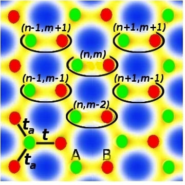
Figure 1: Honeycomb photonic lattice structure with intra-dimer coupling ${t}$ and inter-dimer coupling ${t_{a}=1}$. Sub- lattice (lossy waveguide) $a_{n,m}$ is shown by green circles while sub-lattice (gain waveguide) $b_{n,m}$ is shown by the red circles. Each dimer is distinguished by index ${n}$ and ${m}$. The field is coupled evanescently between the waveguides.

II Photonic Lattice Model

We consider a two dimensional honeycomb photonic lattice of coupled optical waveguides. Each waveguide supports only one mode, while light is transferred from waveguide to waveguide through optical tunneling. A schematic of the set-up is shown in Fig. 1. The lattice consist of two types of waveguides: type (A) made from lossy material (green) whereas type (B) exhibits the equal amount of gain (red). Their arrangement in space is such that they form coupled (A-B) dimers with inter and intra-dimer couplings $t_{a}$ and $t$ respectively. Such structure, apart from a global ${\cal PT}$ symmetry, respects also another anti-linear symmetry (in Ref. BFKS10 we coined this ${\cal P}_{d}{\cal T}$-symmetry) which is related with the local ${\cal PT}$-symmetry of each individual dimer.

Without loss of generality we rescale everything in units of the inter-dimer coupling $t_{a}=1$. In the tight binding description, the diffraction dynamics of the mode electric field amplitude $\Psi_{n,m}=(a_{n,m},b_{n,m})^{T}$ at the $(n,m)-$th dimer evolves according to the following Schrödinger-like equation

$$\begin{array}[]{lcr}i{da_{n,m}\over dz}+\epsilon a_{n,m}+b_{n-1,m+1}+b_{n-1,m-1}+tb_{n,m}&=&0\\ i{db_{n,m}\over dz}+\epsilon^{*}b_{n,m}+a_{n+1,m+1}+a_{n+1,m-1}+ta_{n,m}&=&0\end{array}$$ (1)

where $\epsilon=\epsilon_{0}+i\gamma$ is related to the refractive index MGCM08a . Without loss of generality, we assume $\epsilon_{0}=0$ and $\gamma>0$.

For latter purposes, it is useful to work in the momentum space. To this end, we write the field amplitudes $\Psi_{n,m}$ in their Fourier representation i.e.

$$\begin{array}[]{lcr}a_{n,m}(z)&=&{1\over(2\pi)^{2}}\int_{-\pi}^{\pi}dk_{x}dk_{y}{\tilde{a}}_{k_{x},k_{y}}(z)\exp(i[nk_{x}+mk_{y}])\\ b_{n,m}(z)&=&{1\over(2\pi)^{2}}\int_{-\pi}^{\pi}dk_{x}dk_{y}{\tilde{b}}_{k_{x},k_{y}}(z)\exp(i[nk_{x}+mk_{y}]).\end{array}$$ (2)

Substitution of Eq. (2) to Eq. (1) leads to the following set of coupled differential equations in the momentum space

$$i{d\over dz}\left(\begin{array}[]{c}{\tilde{a}}_{\mathbf{k}}(z)\\ {\tilde{b}}_{\mathbf{k}}(z)\end{array}\right)=H_{\mathbf{k}}\left(\begin{array}[]{c}{\tilde{a}}_{\mathbf{k}}(z)\\ {\tilde{b}}_{\mathbf{k}}(z)\end{array}\right)$$ (3)

where

$$\quad H_{\mathbf{k}}=\left(\begin{array}[]{cc}-i\gamma&D({\mathbf{k}})\\ D({\mathbf{k}})^{*}&i\gamma\end{array}\right).$$ (4)

and

$$D(\mathbf{k})=-(t+2e^{-ik_{x}}\cos k_{y});{\mathbf{k}}\equiv(k_{x},k_{y})$$ (5)

In other words, because of the translational invariance of the system, the equations of motion in the Fourier representation break up into $2\times 2$ blocks, one for each value of momentum ${\bf k}$. The two-component wave functions for different ${\bf k}$ values are then decoupled, thus allowing for a simple theoretical description of the system.

III Eigenmodes Analysis

We start our analysis with the study of the stationary solutions corresponding to the Eq. (3). Substituting the stationary form

$$({\tilde{a}}_{n,m},{\tilde{b}}_{n,m})^{T}=\exp(-i{\cal E}z)(A,B)^{T}$$ (6)

in Eq. (3) we get

$${\cal E}\left(\begin{array}[]{c}A\\ B\end{array}\right)=H_{\mathbf{k}}\left(\begin{array}[]{c}A\\ B\end{array}\right)$$ (7)

The spectrum is obtained by requesting a non-trivial solution i.e. $(A,B)\neq 0$. The corresponding dispersion relation SRBS11 has the form

$${\cal E}_{\pm}=\pm\sqrt{|D({\mathbf{k}})|^{2}-\gamma^{2}}$$ (8)

For $\gamma=0$ the dispersion relation is

$${\cal E}=\pm\left|D({\mathbf{k}})\right|$$ (9)

and we have two bands of width $t+2$. There are three pairs of diabolic points,

$$\begin{array}[]{l}\mathbf{k}^{\pm,\mp}_{0}=(\pm\pi,\pm\arccos{\frac{t}{2}})\\ \mathbf{k}^{\pm}_{1}=(0,\pm(\pi-\arccos{\frac{t}{2}}))\end{array}$$ (10)

Expansion of $D(\mathbf{k})$ up to the first order around the DPs leads to

$$D({\mathbf{k}})\approx it\eta_{x}\mp\sqrt{4-t^{2}}\eta_{y}.$$ (11)

Substituting the above expression in the energy dispersion given by Eqn. (8), we get the following linear relation

$${\cal E}_{\mathbf{k}}\approx\pm(t^{2}\eta_{x}^{2}+(4-t^{2})\eta_{y}^{2})^{1/2}$$ (12)

where $\eta_{x,y}=k_{x,y}-(k_{0,1})_{x,y}$.

The standard passive ($\gamma=0$) honeycomb lattice (zero strain) corresponds to $t=1$. In this case, there are three pairs of DPs at (see Fig.2-a)

$$\begin{array}[]{l}\mathbf{k}^{\pm,\mp}_{0}=(\pm\pi,\pm\frac{\pi}{3})\\ \mathbf{k}^{\pm}_{1}=(0,\pm\frac{2\pi}{3})\end{array}$$ (13)

For $1<t<2$ the two pairs of DPs at $\mathbf{k}^{\pm,\mp}_{0}$ start moving toward each other while the pair at $\mathbf{k}^{\pm}_{1}$ moves away from one another. At $t=2$ a degeneracy occurs i.e. $\mathbf{k}^{\pm,\mp}_{0}=(\pm\pi,0)$. At the same time the dispersion relation ${\cal E}$ around $\mathbf{k}^{\pm,\mp}_{0}$ and $\mathbf{k}^{\pm}_{1}$, is linear only in the $k_{x}$ direction (and quadratic in the $k_{y}$). For $t>2$ the two energy surfaces move away from each other and a gap between them is created (see Fig. 2-b). Therefore for $t\geq 2$ the DPs disappeared for $\gamma=0$, and the conical diffraction is destroyed T08 ; note1 .

By introducing gain/loss to the system described by Eq. (1) the resulting effective Hamiltonian which describes the paraxial evolution becomes non-Hermitian. In fact, for $1\leq t\leq 2$, any value of $\gamma$ results in complex eigenvalues, i.e. the system is in the broken ${\cal PT}$-symmetry phase. The resulting dispersion relation, resembles the dispersion relation of relativistic particles with imaginary mass as was recently discussed in Ref. SRBS11 .

In the case of $t>2$ the size of the gap between the two bands can be controlled by manipulating the gain/loss parameter $\gamma$. In this case, there is a $\gamma$ domain, corresponding to the exact phase, for which the energies are real. It turns out from Eq. (8) that the line

$$\gamma_{\cal PT}=t-2$$ (14)

defines the phase transition from exact to broken ${\cal PT}$-symmetry SRBS11 . The mechanism for this symmetry breaking is the crossing between levels, associated to the exceptional points

$$\begin{array}[]{l}\mathbf{k}^{\pm}_{EP}=(0,\pm\pi)\\ \quad\quad\text{or}\\ \mathbf{k}^{\pm}_{EP}=(\pm\pi,0)\end{array}$$ (15)

(see Fig.2-c) and belonging to different bands BFKS10 : it follows from Eq. (8), that when $\gamma=\gamma_{\cal PT}$, the gap disappears and the two (real) levels at the ”inner” band-edges become degenerate. Evaluation of $D(k_{x},k_{y})$ to second order in $(\eta_{x},\eta_{y})$ around the degeneracy points, leads to

$$D(\eta_{x},\eta_{y})\approx-(\gamma_{\cal PT}+2i\eta_{x}+\eta^{2});\quad\eta^{2}\equiv\eta_{x}^{2}+\eta_{y}^{2}$$ (16)

thus resulting in the following dispersion relation

$${\cal E}=\pm\sqrt{2\gamma_{\cal PT}\eta_{y}^{2}+(2\gamma_{\cal PT}+4)\eta_{x}^{2}}.$$ (17)

For large $\gamma_{\cal PT}$-values (i.e. $\gamma_{\cal PT}\gg 2$) one can approximate the above equation to get

$${\cal E}\approx\pm\sqrt{2\gamma_{\cal PT}}\eta.$$ (18)

This comment will become important in the analysis of optical beam propagation discussed in the next section IV.

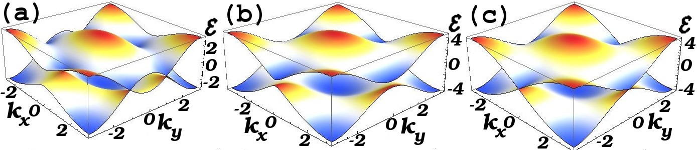
Figure 2: Energy surfaces for a honeycomb lattice with $t_{a}=1$ and (a) $(t,\gamma)=(1,0)$ where a DP is present; (b) $(t,\gamma)=(2.5,0)$ where a band-gap has been created and (c) $(t,\gamma)=(2.5,0.5)$ where a gain/loss parameter led to the creation of a EP.

Next, we turn to the analysis and characterization of the bi-orthogonal set of eigenvectors of our non-Hermitian system. The target here is to identify the proximity to the exceptional point in the case of finite Hilbert spaces, where finite size effects might play an important role in the analysis of the dynamics. The latter do not respect the standard (Euclidian) ortho-normalization condition. Let $\langle L_{n}|$ and $|R_{n}\rangle$ denote the left and right eigenvectors of the non-hermitian Hamiltonian ${\cal H}$ corresponding to the eigenvalue ${\cal E}_{n}$, i.e.

$$\left\{\begin{array}[]{l}\langle L_{n}|{\cal H}=\langle L_{n}|{\cal E}_{n}\\ \quad\quad\text{ and}\\ {\cal H}|R_{n}\rangle={\cal E}_{n}|R_{n}\rangle.\end{array}\right.$$ (19)

The vectors can be normalized to satisfy

$$\left\langle L_{n}|R_{m}\right\rangle=\delta_{nm}$$ (20)

while

$$\sum_{n}^{\cal N}\left|R_{n}\right\rangle\left\langle L_{n}\right|=1$$ (21)

Above ${\cal N}$ is the dimension of the Hilbert space.

An observable that measures the non-orthogonality of the modes, and can be used in order to identify the proximity to the EP in the presence of finite size effects, is the so-called Petermann factor which is defined as Petermann79

$$K_{nm}=\left\langle L_{n}|L_{m}\right\rangle\left\langle R_{m}|R_{n}\right\rangle$$ (22)

We have studied the mean (diagonal) Petermann factor

$$\overline{K}=\frac{1}{\cal N}\sum_{n=1}^{\cal N}K_{nn}$$ (23)

which takes the value $1$ if the eigenfunctions of the system are orthogonal while is larger than one in the opposite case. At the EP, a pair of eigenvectors associated with the corresponding degenerate eigenvalues coalesce, leading to a collapse of the Hilbert space. At this point, the Petermann factor diverges as

$$\overline{K}\sim 1/|\gamma-\gamma_{\cal PT}|$$ (24)

Berry03 ; ZCFK10 . This indicates strong correlations between the spectrum and the eigenvectors which can affect drastically the dynamics as we will see later.

In Figs. 3a-c we present our calculations for $\overline{K}$ for different $(t,\gamma)$ values and various system sizes. We find that as ${\cal N}$ increases the divergence is approaching the line $\gamma_{\cal PT}=t-2$, which was derived previously (see Eq. (14) above) for the case of infinite graphene.

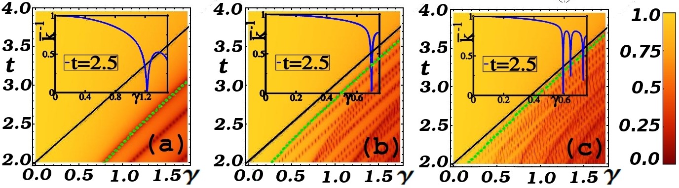
Figure 3: Inverse Petermann factor for various system sizes (a) ${\cal N}=24$; (b) ${\cal N}=168$; (c) ${\cal N}=440$ . The asymptotic line $\gamma_{\cal PT}=t-2$ (black line) is approached by our numerical data (zero of $\overline{K}^{-1}$) for increasing ${\cal N}$. The green line is plotted in order to guide the eye. The insets show representative $\overline{K}^{-1}$’s vs. $\gamma$ for a fixed coupling $t=2.5$.

IV Dynamics

Armed with the previous knowledge about the eigenmodes properties of the ${\cal PT}$-symmetric graphene, we are now ready to study beam propagation in $\cal{PT}$-symmetric honeycomb lattices at the vicinity of the EPs. The question at hand is whether the collapse of the Hilbert space at the EP, will affect the CD pattern, and if yes, what is the emerging dynamical picture.

IV.1 Numerical Analysis

We first study wave propagation in the honeycomb lattice numerically (Fig. 4), by launching a beam with the structure of a Bloch mode associated with the EP, multiplied by a Gaussian envelope. The Bloch modes at the tip can be constructed from pairs of plane waves with ${\mathbf{k}}$ vectors of opposite pairs of exceptional points. Thus, interfering two plane-waves at angles associated with opposite EP yields the phase structure of the modes from these points. Multiplying these waves by an envelope yields a superposition of Bloch modes in a region around these points. Figure 4 shows an example of the propagation of a beam constructed to excite a Gaussian superposition of Bloch modes around an EP. The input beam has a bell-shape structure, which, after some distance, transforms into the ring-like characteristic of conical diffraction note1 . From there on, the ring is propagating in the lattice by keeping its width constant while its radius is increasing linearly with distance. The invariance of the ring thickness and structure manifests a (quasi-) linear dispersion relation above and below the EP (see Fig. 2); hence, the diffraction coefficient for wave packets constructed from Bloch modes in that region is zero (infinite effective mass). This is especially interesting because the ring itself is a manifestation of the dispersion properties at the EP itself, where the diffraction coefficient is infinite (zero-effective mass). As a result, the ring forms a light cone in the lattice. The appearance of CD in the case of ${\cal PT}$-lattices where the eigenvectors are non-orthogonal and coalesce at the EP singularity, provides a clear indication that the phenomenon is insensitive to the eigenmodes structure and it depends only on the properties of the dispersion relation.

The ${\cal PT}$-symmetric conical diffraction shows some unique characteristics with respect to the CD found in the case of beam propagation around DPs for passive honeycomb lattices (i.e. $\gamma=0$). A profound difference is associated with the fact that now, the transverse speed of the cone is increased SRBS11 and in fact it can be controlled by the magnitude of the gain/loss parameter at the symmetry breaking point $\gamma_{\cal PT}$. This is shown in Fig. 4 where we compare the spreading of a CD for two different $\gamma_{\cal PT}$-values.

In Figure 5, we report in a double logarithmic plot, our numerical measurements for the transverse velocity of the spreading ring for various $\gamma_{\cal{PT}}$ values. The best linear fitting to the numerical data shows that transverse speed of the cone is proportional to $\sqrt{\gamma_{\cal PT}}$. This behavior, can be understood qualitatively by realizing that the group velocity near the EP’s is

$$v_{g}=\partial{\cal E}/\partial\mathbf{k}\sim\sqrt{2\gamma_{\cal PT}}$$ (25)

(see Eq. (17) and Eq.(18)). At the same time we find that the resulting ${\cal PT}$-cone is brighter with respect to the one found in passive lattices P07 (i.e. the field intensity of the conical wavefront is larger) .

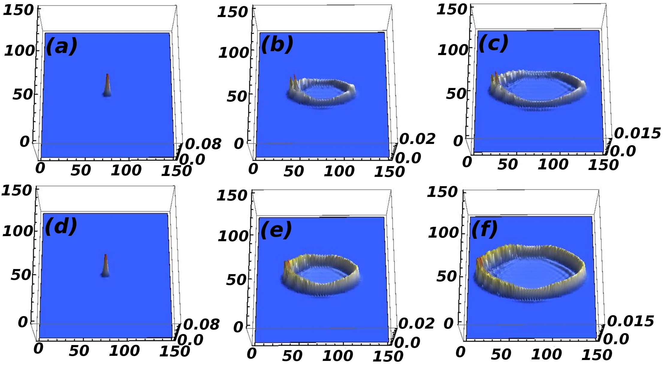
Figure 4: Propagation of a Gaussian superposition of Bloch modes associated with the vicinity of an EP at ${\mathbf{k}}=(0,\pm\pi)$, in a ${\cal PT}$ -symmetric honeycomb lattice. Shown is the beam intensity at normalized propagation distances of (a,d) $z=0$; (b,e)$z=10$; (c,f) $z=15$, for $\gamma_{\cal PT}=1$ and $t=3$ (upper panels) and $\gamma_{\cal PT}=2$ and $t=4$ (lower panels). The input bell-shaped beam transforms into a ring-like structure of light of a non-varying thickness.

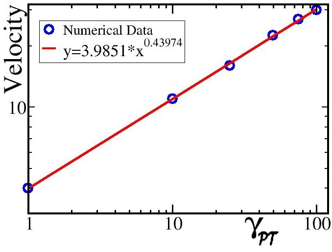
Figure 5: Transverse velocity of the spreading ring versus the $\gamma_{\cal{PT}}$. Numerical simulation approve theoretical prediction for the transverse speed of the CD, which is $v_{g}\propto\sqrt{\gamma_{\cal PT}}$.

IV.2 Theoretical Considerations

It is possible to gain valuable insight into the features of ${\cal PT}$-conical diffraction by considering the field evolution in the momentum space. We consider for simplicity, an initial distribution $({\tilde{a}}_{\mathbf{k}}(0),{\tilde{b}}_{\mathbf{k}}(0))^{T}$ that is symmetric around the EP while it decays exponentially away from it. Specifically we assume

$$({\tilde{a}}_{\mathbf{k}}(0),{\tilde{b}}_{\mathbf{k}}(0))^{T}=e^{-g\sqrt{\eta_{x}^{2}+\eta_{y}^{2}}}(1,0)^{T}.$$ (26)

Next, we calculate the evolution matrix $\mathbf{U}\equiv e^{-i\mathbf{H_{k}}z}$ where $\mathbf{H_{k}}$ is given by Eq. (4). After a straightforward algebra and using the fact that

$$\mathbf{H_{k}}^{2}={\cal E}^{2}\times\mathbf{1},$$ (27)

where $\mathbf{1}$ is the unity matrix, we get

$$\mathbf{U}=\cos(z|{\cal E}|)\mathbf{1}-i(\sin(z|{\cal E}|)/|{\cal E}|)\mathbf{H_{k}}$$ (28)

Equation (28) is the starting point of our analysis. Substituting Eqs. (4,16, 17), we find that the evolving amplitude of the field $(a_{n,m},b_{n,m})$ is

$$a_{n,m}(z) \approx \sum_{l=1,2}\frac{(-1)^{l}i\left[z-\gamma_{\cal PT}\phi(n,m,z,g)\right]+g}{\phi(n,m,z,g)^{3/2}}$$ (29)

$$b_{n,m}(z) \approx \sum_{l=1,2}\frac{(-1)^{l+1}\left(\gamma_{\cal PT}\phi(n,m,z,g)+\frac{n}{\sqrt{2\gamma_{\cal PT}+4}}\right)}{\phi(n,m,z,g)^{3/2}}$$

where

$$\phi(n,m,z,g)=\left[g+(-1)^{l}iz\right]^{2}+n^{2}/(2\gamma_{\cal PT}+4)+m^{2}/(2\gamma_{\cal PT}).$$ (30)

Although our simplified calculations are not able to capture all the features of the propagating cone, the above expression encompasses the main characteristics of the conical diffraction that we have observed in our numerical simulations. At $z=0$, Eq. (29) resembles a Lorentzian, which slowly transforms into a ring of light, whose radius expands linearly with $z$ with velocity $\sqrt{2\gamma_{\cal PT}}$, while its thickness remains unchanged. At the same time the field intensity on the ring in the case of ${\cal PT}$-symmetric lattices is brighter than the one corresponding to passive honeycomb lattices (i.e. $1/z^{2}$ vs $1/z^{4}$ behavior respectively).

V Summary and Concluding Remarks

We studied numerically and analytically the propagation of waves in ${\cal PT}$-honeycomb photonic lattices, demonstrating the existence of conical diffraction arising solely from the presence of a spontaneous ${\cal PT}$-symmetry breaking phase transition point. In spite the fact that the eigenvectors are non-orthogonal and there is a collapse of the Hilbert space at the EP, the emerging cone, is brighter and moves faster than the corresponding one of the passive structure. Although, the realization of such photonic structures is currently a challenging task, active electronic circuits, like the one proposed in Ref. SLZEK11 , can be proven useful alternatives that might allow us to investigate experimentally, wave propagation in extended ${\cal PT}$-symmetric lattices.

These findings raise several intriguing questions. For example, how does nonlinearity affect ${\cal PT}$-symmetric conical diffraction? What is the effect of disorder BFKS09 ? Is this behavior generic for any system at the spontaneously ${\cal PT}$-symmetry breaking point? These intriguing questions are universal, and relate to any field in which waves can propagate in a periodic potential. It is expected that in active metamaterials such phenomena will be present and they may have specific technological importance.

- (1) M. V. Berry and M. R. Jeffrey, Prog. Opt. 50, 13 (2007); M. V. Berry, M. R. Jeffrey, and J. G. Lunney, Proc. R. Soc. London, Ser. A 462, 1629 (2006).
- (2) R. A. Indik and A. C. Newell, Opt. Express 14, 10614 (2006).
- (3) W. R. Hamilton, Trans. R. Irish Acad. 17, 1 (1837).
- (4) H. Lloyd, Trans. R. Irish Acad. 17, 145 (1837).
- (5) O. Peleg et al., Phys. Rev. Lett. 98, 103901 (2007)
- (6) O. Bahat-Treidel et al., Opt. Lett. 33, 2251 (2008)
- (7) M. J. Ablowitz, S. D. Nixon, Y. Zhu, Phys. Rev. A 79, 053830 (2009); M. J. Ablowitz, Y. Zhu Phys. Rev. A 82, 013840 (2010).
- (8) R. I. Egorov et al., Opt. Lett. 31, 2048 (2006).
- (9) O. Bahat-Treidel, O. Peleg, M. Grobman, N. Shapira, M. Segev, and T. Pereg-Barnea, Phys. Rev. Lett. 104, 063901 (2010).
- (10) A. Szameit et al., Phys. Rev. A 84, 021806 (2011).
- (11) K. G. Makris et. al, Phys. Rev. Lett. 100, 103904 (2008).
- (12) T. Kottos, Nature Physics 6, 166 (2010).
- (13) C. M. Bender, S. Boettcher, Phys. Rev. Lett. 80, 5243 (1998); C. M. Bender, D. C. Brody, H. F. Jones, Phys. Rev. Lett. 89, 270401 (2002).
- (14) M. Znojil, Phys. Lett. A 285, 7 (2001); H. F. Jones, J. Phys. A 42, 135303 (2009).
- (15) C. M. Bender, Rep. Prog. Phys. 70, 947 (2007); C. M. Bender et. al, Phys. Rev. Lett. 98, 040403 (2007).
- (16) C. E. Ruter et. al, Nat. Phys. 6, 192 (2010).
- (17) A. Guo, et. al., Phys. Rev. Lett. 103, 093902 (2009).
- (18) J. Schindler, et. al, Phys. Rev. A 84, 040101(R) (2011).
- (19) L. Feng, M. Ayache, J. Huang, Y.-L. Xu, M.-H. Lu, Y.-F. Chen, Y. Fainman, A. Scherer, Science 333, 729 (2011)
- (20) M. C. Zheng et. al, Phys. Rev. A 82, 010103 (2010).
- (21) H. Jones and E. M. Gräfe, Phys. Rev. A (2011).
- (22) S. Longhi, Phys. Rev. Lett. 103, 123601 (2009).
- (23) Z. Lin, et. al, Phys. Rev. Lett 106, 213901 (2011)
- (24) H. Ramezani et. al, Phys. Rev. A 82, 043803 (2010)
- (25) S. Longhi, Phys. Rev. A 82, 031801 (2010); Y. D. Chong, L. Ge, A. D. Stone, Phys. Rev. Lett. 106, 093902 (2011)
- (26) F. Nazari, M. Nazari, M. K. Moravvej-Farshi, Opt. Lett. 36, 4368-4370 (2011).
- (27) A. A. Sukhorukov, Z. Xu, Y. S. Kivshar, Phys. Rev. A 82, 043818 (2010).
- (28) Z. H. Musslimani et. al, Phys. Rev. Lett. 100, 030402 (2008).
- (29) A. Mostafazadeh, J. Math. Phys. 43, 205 (2002)
- (30) A. Mostafazadeh, J. Math. Phys. 43, 3944 (2002)
- (31) A. Mostafazadeh, J. Phys. A 41, 055304 (2008)
- (32) C. M. Bender, M. V. Berry, A. Mandilara, J. Phys. A 35, L467 (2002).
- (33) O. Bendix et al., J. Phys. A: Math. Theor. 43, 265305 (2010).
- (34) Here we use the term ”conical” diffraction in a rather loose fashion. Specifically, when the lattice is deformed i.e. , the CD pattern becomes elliptic T08 .
- (35) K. Petermann, IEEE J. Quantum Electron. 15, 566 (1979); A. E. Siegman, Phys. Rev. A 39, 1264 (1989).
- (36) M. V. Berry, Journal of Modern Optics 50, 63 (2003); S.-Y. Lee et al., Phys. Rev. A 78, 015805 (2008).
- (37) O. Bendix, et. al, Phys. Rev. Lett. 103, 030402 (2009); C. T. West, T. Kottos, T. Prosen, ibid. 104, 054102 (2010).