Towards a renormalization theory for quasi-periodically forced one dimensional maps III. Numerical Support

Abstract

In a previous work by the authors the one dimensional (doubling) renormalization operator was extended to the case of quasi-periodically forced one dimensional maps. The theory was used to explain different self-similarity and universality observed numerically in the parameter space of the Forced Logistic Maps. The extension proposed was not complete in the sense that we assumed a total of four conjectures to be true. In this paper we present numerical support for these conjectures. We also discuss the applicability of this theory to the Forced Logistic Map.

1 Introduction

This is the third of a series of papers (together with [22] and [23]) proposing an extension of the one dimensional renormalization theory for the case of quasi-periodically forced one dimensional maps. These three papers are closely related but each of them has been written to be readable independently. See also [20] for a more detailed discussion. In the previous two papers we were concerned with the theoretical part of the theory. In this paper we include different numerical computations which support the conjectures introduced for the developing of this theory. To do that we briefly review the theory developed in the previous two papers, skipping technical details and we adding some numerical computations to the discussion.

The universality and self-renormalization properties in the cascade of period doubling bifurcations of families of unimodal maps is a well known phenomenon. The paradigmatic example is the Logistic map $l_{\alpha}(x)=\alpha x(1-x)$. Given a typical one parametric family of unimodal maps $\{f_{\alpha}\}_{\alpha\in I}$ one observes numerically that there exists a sequence of parameter values $\{d_{n}\}_{n\in\mathbb{N}}\subset I$ such that the attracting periodic orbit of the map undergoes a period doubling bifurcation. Between one period doubling and the next one there exists also a parameter value $s_{n}$, for which the critical point of $f_{s_{n}}$ is a periodic orbit with period $2^{n}$. One can observe numerically that

$$\lim_{n\rightarrow\infty}\frac{d_{n}-d_{n-1}}{d_{n+1}-d_{n}}=\lim_{n\rightarrow\infty}\frac{s_{n}-s_{n-1}}{s_{n+1}-s_{n}}=\text{\boldmath$\delta$}=\texttt{ 4.66920...}.$$ (1)

This convergence indicates a self-similarity on the parameter space of the family. On the other hand, the constant $\delta$ is universal, in the sense that for any family of unimodal maps with a quadratic turning point having a cascade of period doubling bifurcations, one obtains the same ratio $\delta$.

To explain these phenomena Collet and Treser ([26]) and Feigenbaum ([5, 6]) proposed simultaneously the renormalization operator. Their explanation was based on the existence of a hyperbolic fixed point of the operator with suitable properties. The first proof of the existence of this point and its hyperbolicity were obtained with numerical assistance [15, 4]. A decade later, Sullivan (see [25]) generalized the operator and provided a theoretical proof of the hyperbolicity using complex dynamics techniques. See [17, 3] for extensive summaries on the theory.

In [21] we presented numerical evidences of self similarity and universality for families of quasi-periodically forced Logistic maps. These are maps in the cylinder where the dynamics on the periodic variable are given by a rigid rotation and the dynamics on the other variable are given by the Logistic Map plus a small perturbation which depends on both variables. This kind of maps have its origins in studies related to the existence of strange non-chaotic attractors (see [1, 7, 8, 9, 10, 19]). Let us describe these numerical evidences with more detail.

1.1 Numerical evidence of self-similarity and universality for quasi-periodic forced maps

aaaaa

Figure 1: Schematic representation of the bifurcations diagram of the Forced Logistic Map, for rotation number equal to $\omega$ (left) and $2\omega$ (right). See the text for more details.

Consider $\{g_{\alpha,\varepsilon}\}_{(\alpha,\varepsilon)\in J\subset\mathbb{R}^{2}}$ a two parametric family of quasi-periodic maps in the cylinder $\mathbb{T}\times\mathbb{R}$ of the form

$$\left.\begin{array}[]{rcl}\bar{\theta}&=&\theta+\omega,\\ \bar{x}&=&\alpha x(1-x)+\varepsilon h(\theta,x),\end{array}\right\}$$ (2)

with $\omega$ a Diophantine number, $\alpha$ and $\varepsilon$ parameters and $h$ a periodic function with respect to $\theta$ which can also depend on $\alpha$ and $\varepsilon$. Recall that the Logistic map $\bar{x}=\alpha x(1-x)$ has a complete cascade of period doubling bifurcations. As before, let $\{d_{n}\}_{n\in\mathbb{N}}\subset I$ denote the parameter values where the attracting periodic orbit undergoes a period doubling bifurcation and $\{s_{n}\}_{n\in\mathbb{N}}\subset I$ the values for which the critical point of $f_{s_{n}}$ is a periodic orbit with period $2^{n}$.

In [11] we computed some bifurcation diagrams in terms of the dynamics of the attracting set. We have taken into account different properties of the attracting set, as the Lyapunov exponent and, in the case of having a periodic invariant curve, its period and its reducibility. The reducibility loss of an invariant curve is not a bifurcation in the classical sense that the attracting set of the map changes dramatically, only the spectral properties of the transfer operator associated to the continuation of that curve does (see [12]). Despite of this, it can be characterized as a bifurcation (see definition 2.3 in [11]). The numerical computations in [11] reveal that the parameter values for which the invariant curve doubles its period are contained in regions of the parameter space where the invariant curve is reducible. These computations also reveal that from every parameter value $(\alpha,\varepsilon)=(s_{n},0)$ two curves of reducibility loss (of the $2^{n}$-periodic invariant curve) are born. This situation is sketched in the left panel of figure 1.

Assume that these two curves can be locally expressed as $(s_{n}+\alpha_{n}^{\prime}(\omega)\varepsilon+O(\varepsilon^{2}),\varepsilon)$ and $(s_{n}+\beta_{n}^{\prime}(\omega)\varepsilon+O(\varepsilon^{2}),\varepsilon)$. In [22] we proved that these curves really exist under suitable hypothesis. We have also given explicit expressions of the slopes $\alpha_{n}^{\prime}(\omega)$ and $\beta_{n}^{\prime}(\omega)$ in terms of the quasi-periodic renormalization operator (introduced there). We only focus on $\alpha_{n}^{\prime}(\omega)$, but the discussion for $\beta_{n}^{\prime}(\omega)$ is completely analogous.

The slopes $\alpha_{n}^{\prime}(\omega)$ can be used for the numerical detection of universality and self-renormalization phenomena. If the bifurcation diagram is self-similar by an affine ratio one should have that $\alpha_{n}^{\prime}(\omega)/\alpha_{n-1}^{\prime}(\omega)$ converges to a constant. In [21] we compute numerically this ratios and we show that this is not true due to the fact that when the period is doubled, the rotation number of the system also is. What we find is that there exists an affine relationship between the bifurcation diagram of the family for rotation number $\omega$ and the bifurcation diagram of the same family for rotation number $2\omega$. This is sketched in figure 1.

Concretely, in [21] we observed numerically the following behavior.

• First numerical observation: the sequence $\alpha_{n}^{\prime}(\omega)/\alpha_{n-1}^{\prime}(\omega)$ is not convergent in $n$. But, for $\omega$ fix, one obtains the same sequence for any family of quasi-periodic forced map like (2), with a quasi-periodic forcing of the type $h(\theta,x)=f_{1}(x)\cos(\theta)$.

• Second numerical observation: the sequence $\alpha_{n}^{\prime}(\omega)/\alpha_{n-1}^{\prime}(2\omega)$ associated to maps like (2) is convergent in $n$ when we take the quasi-periodic forcing of the type $h(\theta,x)=f_{1}(x)\cos(\theta)$. The limit depends on $\omega$ and $f_{1}$.

• Third numerical observation: the two previous observations are not true when the quasi-periodic forcing is of the type $h_{\eta}(\theta,x)=f_{1}(x)\cos(\theta)+\eta f_{2}(x)\cos(2\theta)$ when $\eta\neq 0$. But the sequence $\alpha_{n}^{\prime}(\omega)/\alpha_{n-1}^{\prime}(2\omega)$ associated to the map (2) with $h=h_{\eta}$ is $\eta$-close to the same maps with $h=h_{0}$

In [22] we extended the renormalization operator and we obtained explicit expressions of the slopes $\alpha_{n}^{\prime}(\omega)$ and $\beta_{n}^{\prime}(\omega)$ in terms of the quasi-periodic renormalization operator. This is reviewed in section 2. In [23] we give a theoretical explanation to the numerical observations described above in terms of the dynamics of the quasi-periodic renormalization operator. This is reviewed in section 3. The novelty in this paper is that we present numerical support to the conjectures done in [22, 23]. This numerical support is presented after the statement of each of the conjectures, with the exception of conjecture A, which is given in section 4. In Appendix A we describe the numerical approximation used to discretize the renormalization operator and how we use it to compute the spectrum of its derivative.

2 Existence of reducibility loss bifurcations

Consider a quasi-periodic forced map like

$$\begin{array}[]{rccc}F:&\mathbb{T}\times I&\rightarrow&\mathbb{T}\times I\\ &\left(\begin{array}[]{c}\theta\\ x\end{array}\right)&\mapsto&\left(\begin{array}[]{c}\theta+\omega\\ f(\theta,x)\end{array}\right),\end{array}$$ (3)

with $f\in C^{r}(\mathbb{T}\times I,I)$. To define the renormalization operator it is only necessary that $r\geq 1$, but we restrict this study to the analytic case due to technical reasons. Along section 2.1 it is not necessary to require $\omega$ Diophantine, but it will be necessary in section 2.2.

The definition of the operator is done in a perturbative way, in the sense that it is only applicable to maps $f(\theta,x)=g(x)+h(\theta,x)$ with $g$ renormalizable in the one dimensional sense and $h$ small.

2.1 Definition of the operator and basic properties

Preliminary notation

Let $\mathbb{W}$ be an open set in the complex plane containing the interval $I_{\delta}=[-1-\delta,1+\delta]$ and let $\mathbb{B}_{\rho}=\{z=x+iy\in\mathbb{C}\text{ such that }|y|<\rho\}$. Then consider $\mathcal{B}=\mathcal{B}(\mathbb{B}_{\rho},\mathbb{W})$ the space of functions $f:\mathbb{B}_{\rho}\times\mathbb{W}\rightarrow\mathbb{C}$ such that:

1. $f$ is holomorphic in $\mathbb{B}_{\rho}\times\mathbb{W}$ and continuous in the closure of $\mathbb{B}_{\rho}\times\mathbb{W}$.

2. $f$ is real analytic.

3. $f$ is $1$-periodic in the first variable.

This space endowed with the supremum norm is Banach.

Let $\mathcal{RH}(\mathbb{W})$ denote the space of functions $f:\mathbb{W}\rightarrow\mathbb{C}$ such that are holomorphic in $\mathbb{W}$, continuous in the closure of $\mathbb{W}$, and send real number to real numbers. This space is also Banach with the supremum norm.

Consider the operator

$$\begin{array}[]{rccc}p_{0}:&\mathcal{B}&\rightarrow&\mathcal{RH}(\mathbb{W})\\ \displaystyle\rule{0.0pt}{12.91663pt}&f(\theta,x)&\mapsto&\rule{0.0pt}{12.91663pt}\displaystyle\int_{0}^{1}f(\theta,x)d\theta.\end{array}$$ (4)

Let $\mathcal{B}_{0}$ the natural inclusion of $\mathcal{RH}(\mathbb{W})$ into $\mathcal{B}$. Then we have that $p_{0}$ as a map from $\mathcal{B}$ to $\mathcal{B}_{0}$ is a projection ($(p_{0})^{2}=p_{0}$).

Set up of the one dimensional renormalization operator.

First we give a concrete definition of the one dimensional renormalization operator before extending it to the quasi-periodic case. Actually, this is a minor modification of the one given in [15].

Given a small value $\delta>0$, let $\mathcal{M}_{\delta}$ denote the subspace of $\mathcal{RH}(\mathbb{W})$ formed by the even functions $\psi$ which send the interval $I_{\delta}=[-1-\delta,1+\delta]$ into itself, and such that $\psi(0)=1$ and $x\psi^{\prime}(x)<0$ for $x\neq 0$.

Set $a=\psi(1)$, $a^{\prime}=(1+\delta)a$ and $b^{\prime}=\psi(a^{\prime})$. We can define $\mathcal{D}(\mathcal{R}_{\delta})$ as the set of $\psi\in\mathcal{M}_{\delta}$ such that $a<0$, $1>b^{\prime}>-a^{\prime}$, and $\psi(b^{\prime})<-a^{\prime}$.

We define the renormalization operator, $\mathcal{R}_{\delta}:\mathcal{D}(\mathcal{R}_{\delta})\rightarrow\mathcal{M}_{\delta}$ as

$$\mathcal{R}_{\delta}(\psi)(x)=\frac{1}{a}\psi\circ\psi(ax).$$ (5)

where $a=\psi(1)$.

Note that, given $\psi\in\mathcal{D}(\mathcal{R}_{\delta})$, one needs to ensure that $\psi\left(a\mathbb{W}\right)\subset\mathbb{W}$ in order to have $\mathcal{R}_{\delta}(\psi)$ well defined. With this aim, let us consider the following hypothesis.

H0)

There exists an open set $\mathbb{W}\subset\mathbb{C}$ containing $I_{\delta}$ and a function $\Phi\in\mathcal{B}$such that $\phi=p_{0}(\Phi)$ is a fixed point of the renormalization operator $\mathcal{R}_{\delta}$ and such that the closure of both $a\mathbb{W}$ and $\phi(\Phi)(a\mathbb{W})$ is contained in $\mathbb{W}$ (with $a:=\Phi(1)$).

In [16], Lanford claims that the hypothesis H0 is satisfied by the set

$$\left\{z\in\mathbb{C}\text{ such that }|z^{2}-1|<\frac{5}{2}\right\}.$$ (6)

This set is convenient for him because he works in the set of even holomorphic functions.

In [15] Lanford introduces a discretization of the (one dimensional) renormalization operator to give a computer assisted proof of the contractivity of the operator. In the present paper we use the same techniques to discretize the quasi-periodic renormalization operator, although we do it without the use of rigorous interval arithmetics. More details on this are given in the Appendix A. We can use this discretization to check the hypothesis H0 for a suitable set $\mathbb{W}$.

Figure 2: Boundaries of the sets $\mathbb{D}\left(\frac{1}{5},\frac{3}{2}\right)$ (solid line) and $\phi\left(a\mathbb{D}\left(\frac{1}{5},\frac{3}{2}\right)\right)$ (dashed line).

Our study is not restricted to the case of even functions, therefore the set (6) used by Lanford is not valid in our case. Using the method described in the Appendix A we recomputed the fixed point $\phi$ of the (one dimensional) renormalization operator $\mathcal{R}$. The fixed point has been computed by means of a Newton method with our discretization and then we have checked that the Taylor expansion around zero coincides with the one given in [15].

With this approximation of $\phi$ we checked (numerically) that $\mathbb{D}\left(\frac{1}{5},\frac{3}{2}\right)$ the disc of the complex plane centered at $\frac{1}{5}$ with radius $\frac{3}{2}$ satisfies the conditions required to the set $\mathbb{W}$ in hypothesis H0. In other words, we checked that $\phi\left(a\mathbb{D}\left(\frac{1}{5},\frac{3}{2}\right)\right)$ is contained inside $\mathbb{D}\left(\frac{1}{5},\frac{3}{2}\right)$ (recall that $a=\phi(1)$ and $a\mathbb{D}(z_{0},\rho)=\{z\in\mathbb{C}\thinspace|\thinspace az\in\mathbb{D}(z_{0},\rho)\}$ ).

Denote by $\partial\mathbb{D}(z_{0},\rho)$ the boundary of the disk $\mathbb{D}(z_{0},\rho)$. In figure 2 we have plotted the sets $\partial\mathbb{D}\left(\frac{1}{5},\frac{3}{2}\right)$ and $\phi\left(a\partial\mathbb{D}\left(\frac{1}{5},\frac{3}{2}\right)\right)$ which give a visual evidence of the inclusion. Recall that $\phi$ is analytic, then to check that the set $\mathbb{D}\left(\frac{1}{5},\frac{3}{2}\right)$ is mapped inside the set delimited by $\phi\left(a\partial\mathbb{D}\left(\frac{1}{5},\frac{3}{2}\right)\right)$ it is enough to check that one point in the interior of $\mathbb{D}\left(\frac{1}{5},\frac{3}{2}\right)$ is mapped in the interior of $\phi\left(a\partial\mathbb{D}\left(\frac{1}{5},\frac{3}{2}\right)\right)$. Recall that $\phi(0)=1$ by hypothesis, therefore the inclusion holds.

Definition of the renormalization operator for quasi-periodically forced maps

Consider the space $\mathcal{X}\subset\mathcal{B}$ defined as:

$$\mathcal{X}=\{f\in C^{r}(\mathbb{T}\times I_{\delta},I_{\delta})|\thinspace p_{0}(f)\in\mathcal{M}_{\delta}\}.$$

Consider also the decomposition $\mathcal{X}=\mathcal{X}_{0}\oplus\mathcal{X}_{0}^{c}$ given by the projection $p_{0}$. In other words, we have $\mathcal{X}_{0}=\{f\in\mathcal{X}\thinspace|\text{ }p_{0}(f)=f\}$ and $\mathcal{X}^{c}_{0}=\{f\in\mathcal{X}\thinspace|\text{ }p_{0}(f)=0\}$. Note that from the definition of $\mathcal{X}$ it follows that $\mathcal{X}_{0}$ is an isomorphic copy of $\mathcal{M}_{\delta}$.

Given a function $g\in\mathcal{X}$, we define the quasi-periodic renormalization of $g$ as

$$[\mathcal{T}_{\omega}(g)](\theta,x):=\frac{1}{\hat{a}}g(\theta+\omega,g(\theta,\hat{a}x)),$$ (7)

where $\displaystyle\hat{a}=\int_{0}^{1}g(\theta,1)d\theta$.

Then we have that there exists a set $\mathcal{D}(\mathcal{T})$, open in $\left(p_{0}\circ\mathcal{T}_{\omega}\right)^{-1}(\mathcal{M}_{\delta})$, where the operator is well defined. Moreover this set contains $\mathcal{D}_{0}(\mathcal{T})$, the inclusion of $\mathcal{D}(\mathcal{R})$ in $\mathcal{B}$. By definition we have that $\mathcal{T}_{\omega}$ restricted to $\mathcal{D}_{0}(\mathcal{T})$ is isomorphically conjugate to $\mathcal{R}$, therefore the fixed points of $\mathcal{R}$ extend to fixed points of $\mathcal{T}_{\omega}$. Assume that H0 holds and let $\Phi$ be the fixed point given by this hypothesis. Then we have that there exists $U\subset\mathcal{D}(\mathcal{T})\cap\mathcal{B}$, an open neighborhood of $\Phi$, such that $\mathcal{T}_{\omega}:U\rightarrow\mathcal{B}$ is well defined. Moreover we have that $\mathcal{T}_{\omega}$ is Fréchet differentiable for any $\Psi\in U$.

Fourier expansion of $D\mathcal{T}_{\omega}(\Psi)$.

Let $\Psi$ be a function in a neighborhood of $\Phi$ (given in hypothesis H0) where $\mathcal{T}_{\omega}$ is differentiable. Additionally, assume that $\Psi\in\mathcal{D}_{0}(\mathcal{T}_{\omega})$.

Given a function $f\in\mathcal{B}$ we can consider its complex Fourier expansion in the periodic variable

$$f(\theta,z)=\sum_{k\in\mathbb{Z}}c_{k}(z)e^{2\pi k\theta i},$$ (8)

with

$$c_{k}(z)=\int_{0}^{1}f(\theta,z)e^{-2\pi k\theta i}d\theta.$$

Then we have that $D\mathcal{T}_{\omega}$ “diagonalizes” with respect to the complex Fourier expansion, in the sense that we have

$$\left[D\mathcal{T}_{\omega}(\Psi)f\right](\theta,z)=D\mathcal{R}_{\delta}[c_{0}](z)+\sum_{k\in\mathbb{Z}\setminus\{0\}}\left([L_{1}(c_{k})](z)+[L_{2}(c_{k})](z)e^{2\pi k\omega i}\right)e^{2\pi k\theta i},$$ (9)

where

$$\begin{array}[]{rccc}L_{1}:&\mathcal{RH}(\mathbb{W})&\rightarrow&\mathcal{RH}(\mathbb{W})\\ &g(z)&\mapsto&\displaystyle\frac{1}{a}\psi^{\prime}\circ\psi(az)g(az),\end{array}$$

and

$$\begin{array}[]{rccc}L_{2}:&\mathcal{RH}(\mathbb{W})&\rightarrow&\mathcal{RH}(\mathbb{W})\\ &g(z)&\mapsto&\displaystyle\frac{1}{a}g\circ\psi(az),\end{array}$$

with $\psi=p_{0}(\Psi)$ and $a=\psi(1)$.

An immediate consequence of this diagonalization is the following. Consider

$$\mathcal{B}_{k}:=\big{\{}f\in B|\text{ }f(\theta,x)=u(x)\cos(2\pi k\theta)+v(x)\sin(2\pi k\theta),\text{ for some }u,v\in\mathcal{RH}(\mathbb{W})\big{\}},$$ (10)

then we have that the spaces $\mathcal{B}_{k}$ are invariant by $D\mathcal{T}(\Psi)$ for any $k>0$.

Moreover $D\mathcal{T}_{\omega}(\Psi)$ restricted to $\mathcal{B}_{k}$ is conjugate to $\mathcal{L}_{k\omega}$, where $\mathcal{L}_{\alpha}$ is the defined as

$$\begin{array}[]{rccc}\mathcal{L}_{\alpha}:&\mathcal{RH}(\mathbb{W})\oplus\mathcal{RH}(\mathbb{W})&\rightarrow&\mathcal{RH}(\mathbb{W})\oplus\mathcal{RH}(\mathbb{W})\\ \\ &\left(\begin{array}[]{c}u\\ v\end{array}\right)&\mapsto&\left(\begin{array}[]{c}L_{1}(u)\\ L_{1}(v)\end{array}\right)+\left(\begin{array}[]{cc}\cos(2\pi\alpha)&-\sin(2\pi\alpha)\\ \sin(2\pi\alpha)&\cos(2\pi\alpha)\end{array}\right)\left(\begin{array}[]{c}L_{2}(u)\\ L_{2}(v)\end{array}\right).\end{array}$$ (11)

Then we have that the understanding of the derivative of the renormalization operator in $\mathcal{B}$ is equivalent to the study of the operator $\mathcal{L}_{\omega}$ for a any $\omega\in\mathbb{T}$.

Properties of $\mathcal{L}_{\omega}$

Figure 3: Numerical approximation of the spectrum of $\mathcal{L}_{\omega}$ for $\omega\in\mathbb{T}$. Top: projection in the complex plane of the spectrum when $\omega$ varies in $\mathbb{T}$. Bottom left: evolution of the real part with respect to $\omega$. Bottom right: evolution of the imaginary part with respect to $\omega$.

Given a value $\gamma\in\mathbb{T}$, consider the rotation $R_{\gamma}$ defined as

$$\begin{array}[]{rccc}R_{\gamma}:&\mathcal{RH}(\mathbb{W})\oplus\mathcal{RH}(\mathbb{W})&\rightarrow&\mathcal{RH}(\mathbb{W})\oplus\mathcal{RH}(\mathbb{W})\\ \\ &\left(\begin{array}[]{c}u\\ v\end{array}\right)&\mapsto&\left(\begin{array}[]{cc}\cos(2\pi\gamma)&-\sin(2\pi\gamma)\\ \sin(2\pi\gamma)&\cos(2\pi\gamma)\end{array}\right)\left(\begin{array}[]{c}u\\ v\end{array}\right),\end{array}$$ (12)

then we have that $\mathcal{L}_{\omega}$ and $R_{\gamma}$ commute for any $\omega,\gamma\in\mathbb{T}$.

This has some consequences on the spectrum of $\mathcal{L}_{\omega}$. Concretely, we have that any eigenvalue of $\mathcal{L}_{\omega}$ (different from zero) is either real with geometric multiplicity even, or a pair of complex conjugate eigenvalues. On the other hand $\mathcal{L}_{\omega}$ depends analytically on $\omega$, which (using theorems III-6.17 and VII-1.7 of [13]) imply that (as long as the eigenvalues of $\mathcal{L}_{\omega}$ are simple) the eigenvalues and their associated eigenspaces depend analytically on the parameter $\omega$.

Finally, doing some minor changes on the domain of definition, we can prove the compactness of the operator $\mathcal{L}_{\omega}$. Recall that the compactness of an operator implies that its spectrum is either finite or countable with $0$ on its closure (see for instance theorem III-6.26 of [13]).

In figure 3 we have a numerical approximation of the spectrum of the operator $\mathcal{L}_{\omega}$ depending on $\omega$. We can observe that the properties described above are satisfied. The details on the numerical computations involved to approximate the spectrum are described in Appendix A. Several numerical tests on the reliability of the results are also included there.

2.2 Reducibility loss and quasi-periodic renormalization

Given a map $F$ like (3) with $f\in\mathcal{B}$ and $\omega\in\mathbb{T}$, we denote by $f^{n}:\mathbb{T}\times\mathbb{R}\rightarrow\mathbb{R}$ the $x$-projection of $F^{n}(x,\theta)$. Equivalently $f^{n}$ can be defined through the recurrence

$$f^{n}(\theta,x)=f(\theta+(n-1)\omega,f^{n-1}(\theta,x)),\quad f^{0}(\theta,x)\equiv x.$$ (13)

From this point on, whenever $\omega$ is used, it is assumed to be Diophantine. Denote by $\Omega=\Omega_{\gamma,\tau}$ the set of Diophantine numbers, this is the set of $\omega\in\mathbb{T}$ such that there exist $\gamma>0$ and $\tau\geq 1$ such that

$$|q\omega-p|\geq\frac{\gamma}{|q|^{\tau}},\quad\text{ for all }(p,q)\in\mathbb{Z}\times(\mathbb{Z}\setminus\{0\}).$$

Additionally, we will need to assume that the following conjecture is true.

Conjecture A.

The operator $\mathcal{T}_{\omega}$ (for any $\omega\in\Omega$) is an injective function when restricted to the domain $\mathcal{B}\cap\mathcal{D}(\mathcal{T})$. Moreover, there exists $U$ an open set of $\mathcal{D}(\mathcal{T})$ containing $W^{u}(\Phi,\mathcal{R})\cup W^{s}(\Phi,\mathcal{R})$ where the operator $\mathcal{T}_{\omega}$ is differentiable.

In [22] we discuss the difficulties for proving this conjecture. A priory there is no way to check numerically this kind of conjecture. A posteriori we have that the results obtained assuming this conjecture are coherent with the numerical computations (see section 4).

Consequences for a two parametric family of maps

Consider a two parametric families of maps $\{c(\alpha,\varepsilon)\}_{(\alpha,\varepsilon)\in A}$ contained in $\mathcal{B}$, with $A=[a,b]\times[0,c]$ and $a$, $b$ and $c$ are real numbers (with $a<b$ and $0<c$). We assume that the dependency on the parameters is analytic.

Consider the following hypothesis on the family of maps.

H1)

The family $\{c(\alpha,\varepsilon)\}_{(\alpha,\varepsilon)\in A}$ uncouples for $\varepsilon=0$, in the sense that the family $\{c(\alpha,0)\}_{\alpha\in[a,b]}$ does not depend on $\theta$ and it has a full cascade of period doubling bifurcations. We assume that the family $\{c(\alpha,0)\}_{\alpha\in[a,b]}$ crosses transversally the stable manifold of $\Phi$, the fixed point of the renormalization operator, and each of the manifolds $\Sigma_{n}$ for any $n\geq 1$, where $\Sigma_{n}$ is the inclusion in $\mathcal{B}$ of the set of one dimensional unimodal maps with a super-attracting $2^{n}$ periodic orbit.

In other words, we assume that the family $c(\alpha,\varepsilon)$ can be written as,

$$c(\alpha,\varepsilon)=c_{0}(\alpha)+\varepsilon c_{1}(\alpha,\varepsilon),$$

with $\{c_{0}(\alpha)\}_{\alpha\in[a,b]}\subset\mathcal{B}_{0}$ having a full cascade of period doubling bifurcations.

Given a family $\{c(\alpha,\varepsilon)\}_{(\alpha,\varepsilon)\in A}$ satisfying the hypothesis H1, let $\alpha_{n}$ be the parameter value for which the uncoupled family $\{c(\alpha,0)\}_{\alpha\in[a,b]}$ intersects the manifold $\Sigma_{n}$. Note that the critical point of the map $c(\alpha_{n},0)$ is a $2^{n}$-periodic orbit. Our main achievement in [22] is to prove that from every parameter value $(\alpha_{n},0)$ there are born two curves in the parameter space, each of them corresponding to a reducibility loss bifurcation. If we want to give a more precise statement of the result we need now to introduce some technical definitions.

Let $\mathcal{RH}(\mathbb{B}_{\rho},\mathbb{W})$ denote the space of periodic real analytic maps from $\mathbb{B}_{\rho}$ to $\mathbb{W}$ and continuous in the closure of $\mathbb{B}_{\rho}$. Consider a map $f_{0}\in\mathcal{B}$ and $\omega\in\Omega$, such that $f$ has a periodic invariant curve $x_{0}$ of rotation number $\omega$ with a Lyapunov exponent less equal than certain $-K_{0}<0$. Using lemma 3.6 in [22] we have that there exist a neighborhood $V\subset\mathcal{B}$ of $f_{0}$ and a map $x\in\mathcal{RH}(\mathbb{B}_{\rho},\mathbb{W})$ such that $x(f)$ is a periodic invariant curve of $f$ for any $f\in V$. Then we can define the map $G_{1}$ as

$$\begin{array}[]{rccc}G_{1}:&\Omega\times V&\rightarrow&\mathcal{RH}(\mathbb{B}_{\rho},\mathbb{C})\\ \rule{0.0pt}{12.91663pt}&(\omega,g)&\mapsto&D_{x}g\big{(}\theta+\omega,g(\theta,\left[x(\omega,g)\right](\theta))\big{)}D_{x}g\big{(}\theta,\left[x(\omega,g)\right](\theta)\big{)}.\end{array}$$ (14)

On the other hand, we can consider the counterpart of the map $G_{1}$ in the uncoupled case. Given a map $f_{0}\in\mathcal{B}_{0}$, consider $U\subset\mathcal{B}_{0}$ a neighborhood of $f_{0}$ in the $\mathcal{B}_{0}$ topology. Assume that $f_{0}$ has a attracting $2$-periodic orbit $x_{0}\in I$. Let $x=x(f)\in\mathbb{W}$ be the continuation of this periodic orbit for any $f\in U$. We have that $x$ depends analytically on the map, therefore it induces a map $x:U\rightarrow\mathbb{W}$. Then if we take $U$ small enough we have an analytic map $x:U\rightarrow\mathbb{W}$ such that $x[f]$ is a periodic orbit of period 2. Now we can consider the map

$$\begin{array}[]{rccc}\widehat{G}_{1}:&U\subset\mathcal{B}_{0}&\rightarrow&\mathbb{C}\\ \rule{0.0pt}{12.91663pt}&f&\mapsto&D_{x}f\big{(}f(x[f])\big{)}D_{x}f\big{(}x[f]\big{)}.\end{array}$$ (15)

Note that $\widehat{G}_{1}$ corresponds to $G_{1}$ restricted to the space $\mathcal{B}_{0}$ (but then $\widehat{G}_{1}(f)$ has to be seen as an element of $\mathcal{RH}(\mathbb{B}_{\rho},\mathbb{W})$).

Consider the sequences

$$\begin{array}[]{rcll}\omega_{k}&=&2\omega_{k-1},&\text{ for }k=1,...,n-1.\\ \rule{0.0pt}{17.22217pt}f^{(n)}_{k}&=&\mathcal{R}\left(f_{k-1}^{(n)}\right),&\text{ for }k=1,...,n-1.\\ \rule{0.0pt}{17.22217pt}u^{(n)}_{k}&=&D\mathcal{R}\left(f^{(n)}_{k-1}\right)u^{(n)}_{k-1},&\text{ for }k=1,...,n-1.\\ \rule{0.0pt}{17.22217pt}v^{(n)}_{k}&=&D\mathcal{T}_{\omega_{k-1}}\left(f^{(n)}_{k-1}\right)v^{(n)}_{k-1},&\text{ for }k=1,...,n-1.\end{array}$$ (16)

with

$$f^{(n)}_{0}=c(\alpha_{n},0),\quad u^{(n)}_{0}=\partial_{\alpha}c(\alpha_{n},0),\quad v^{(n)}_{0}=\partial_{\varepsilon}c(\alpha_{n},0).$$ (17)

Note that $f^{(n)}_{0}=\{c(\alpha,0)\}\cap\Sigma_{n}$, then $f^{(n)}_{0}$ tends to $W^{s}(\mathcal{R},\Phi)$ when $n$ grow. Therefore, the sequence $\{f^{(n)}_{k}\}_{0\leq k<n}$ attains to $W^{s}(\mathcal{R},\Phi)\cup W^{u}(\mathcal{R},\Phi)$ when $n$ grows and consequently there exist $n_{0}$ such that $\{f^{(n)}_{k}\}_{0\leq k<n}\subset U$ , where $U$ is the neighborhood given in conjecture A. If the conjecture is true, then the operator $\mathcal{T}_{\omega}$ is differentiable in the orbit $\{f^{(n)}_{k}\}_{0\leq k<n}\subset U$.

Consider the following hypothesis.

H2)

The family $\{c(\alpha,\varepsilon)\}_{(\alpha,\varepsilon)\in A}$ is such that

$$DG_{1}\left(\omega_{n-1},f^{(n)}_{n-1}\right)D\mathcal{T}_{\omega_{n-2}}\left(f^{(n)}_{n-2}\right)\cdots D\mathcal{T}_{\omega_{0}}\left(f^{(n)}_{0}\right)\partial_{\varepsilon}c(\alpha_{n},0),$$

has a unique non-degenerate minimum (respectively maximum) as a function from $\mathbb{T}$ to $\mathbb{R}$, for any $n\geq n_{0}$.

Consider a family of maps $\{c(\alpha,\varepsilon)\}_{(\alpha,\varepsilon)\in A}$ such that the hypotheses H1 and H2 are satisfied and $\omega_{0}\in\Omega$. If the conjecture A is true, then theorem 3.8 in [22] asserts that there exists $n_{0}$ such that, for any $n\geq n_{0}$, there exist two bifurcation curves around the parameter value $(\alpha_{n},0)$, such that they correspond to a reducibility-loss bifurcation of the $2^{n}$-periodic invariant curve. Moreover, these curves are locally expressed as $(\alpha_{n}+\alpha_{n}^{\prime}(\omega)\varepsilon+o(\varepsilon),\varepsilon)$ and $(\alpha_{n}^{-}+\beta_{n}^{\prime}(\omega)\varepsilon+o(\varepsilon),\varepsilon)$ with

$$\alpha^{\prime}_{n}(\omega)=-\frac{m\left(DG_{1}\left(\omega_{n-1},f^{(n)}_{n-1}\right)v_{n-1}^{(n)}\right)}{\rule{0.0pt}{15.0694pt}D\widehat{G}_{1}\left(f^{(n)}_{n-1}\right)u_{n-1}^{(n)}},$$ (18)

and

$$\beta^{\prime}_{n}(\omega)=-\frac{M\left(DG_{1}\left(\omega_{n-1},f^{(n)}_{n-1}\right)v_{n-1}^{(n)}\right)}{\rule{0.0pt}{15.0694pt}D\widehat{G}_{1}\left(f^{(n)}_{n-1}\right)u_{n-1}^{(n)}},$$ (19)

where $G_{1}$ and $\widehat{G}_{1}$ are given by equations (14) and (15), and $m$ and $M$ are the minimum and the maximum as operators, that is

$$\begin{array}[]{rccc}m:&\mathcal{RH}(\mathbb{B}_{\rho},\mathbb{C})&\rightarrow&\mathbb{R}\\ \rule{0.0pt}{12.91663pt}&g&\mapsto&\displaystyle\min_{\theta\in\mathbb{T}}g(\theta).\end{array}$$ (20)

and

$$\begin{array}[]{rccc}M:&\mathcal{RH}(\mathbb{B}_{\rho},\mathbb{C})&\rightarrow&\mathbb{R}\\ \rule{0.0pt}{12.91663pt}&g&\mapsto&\displaystyle\max_{\theta\in\mathbb{T}}g(\theta).\end{array}$$ (21)

Let us focus again on hypothesis H2, which is not intuitive. We can introduce a stronger condition which much more easy to check. Moreover this conditions is automatically satisfied by maps like the Forced Logistic Map. Consider a family of maps $\{c(\alpha,\varepsilon)\}_{(\alpha,\varepsilon)\in A}$ as before, satisfying hypothesis H1.

H2’)

The family $\{c(\alpha,\varepsilon)\}_{(\alpha,\varepsilon)\in A}$ is such that the quasi-periodic perturbation $\partial_{\varepsilon}c(\alpha,0)$ belongs to the set $\mathcal{B}_{1}$ (see equation (10)) for any value of $\alpha$ (with $(\alpha,0)\in A$).

Then we have that H2’ implies H2 (see proposition 3.10 in [22]).

3 Asymptotic behavior of reducibility loss bifurcations

Consider a two parametric family of maps $\{c(\alpha,\varepsilon)\}_{(\alpha,\varepsilon)\in A}$ contained in $\mathcal{B}$, with $A=[a,b]\times[0,d]$ and $a$, $b$ and $d$ are real numbers (with $a<b$ and $0<d$). We assume that the dependency on the parameters is analytic and the family is such that the hypotheses H1 and H2 introduced in section 2.2 are satisfied. Consider also the reducibility loss bifurcation curves associated to the $2^{n}$-periodic orbit given by (18). Since the value $\alpha_{n}^{\prime}(\omega)$ depends also on the family of maps $c$ considered, we will denote it by $\alpha_{n}^{\prime}(\omega,c)$ from now on. We omit the case concerning $\beta_{n}^{\prime}(\omega)$ (see (19)) because it is completely analogous to the one considered here.

3.1 Rotational symmetry reduction

Given $\gamma\in\mathbb{T}$, consider the following auxiliary function

$$\begin{array}[]{rccc}t_{\gamma}:&\mathcal{B}&\rightarrow&\mathcal{B}\\ \rule{0.0pt}{21.52771pt}&v(\theta,z)&\mapsto&v(\theta+\gamma,z).\end{array}$$ (22)

Let $\mathcal{B}_{1}$ be the subspace of $\mathcal{B}$ defined by (10) for $k=1$. The space $\mathcal{B}_{1}$ is indeed the image of the projection $\pi_{1}:\mathcal{B}\rightarrow\mathcal{B}$ defined as

$$\left[\pi_{1}(v)\right](\theta,x)=\left(\int_{0}^{1}v(\theta,x)\cos(2\pi x)d\theta\right)\cos(2\pi\theta)+\left(\int_{0}^{1}v(\theta,x)\sin(2\pi x)d\theta\right)\sin(2\pi\theta).$$ (23)

Given $x_{0}\in\mathbb{W}\cap\mathbb{R}$ and $\theta_{0}\in\mathbb{T}$ we can also consider the sets

$$\mathcal{B}_{1}^{\prime}=\mathcal{B}_{1}^{\prime}(\theta_{0},x_{0})=\{f\in\mathcal{B}_{1}\thinspace|f(\theta_{0},x_{0})=0,\partial_{\theta}f(\theta_{0},x_{0})>0\},$$

and

$$\mathcal{B}^{\prime}=\mathcal{B}^{\prime}(\theta_{0},x_{0})=\{f\in\mathcal{B}\thinspace|\pi_{1}(f)\in\mathcal{B}_{1}^{\prime}\}.$$

Note that $\mathcal{B}_{1}^{\prime}(\theta_{0},x_{0})$ depends on the election of $(\theta_{0},x_{0})$, but for any fixed $x_{0}$ and $\theta_{0}$ the set $\mathcal{B}_{1}^{\prime}(\theta_{0},x_{0})$ is an open subset of a codimension one linear subspace of $\mathcal{B}_{1}$. Note also that any $v\in$ then $v\neq 0$ due to the condition $\partial_{\theta}v(\theta_{0},x_{0})>0$. Moreover for any $v\in\mathcal{B}_{1}\setminus\{0\}$ there exists a unique $\gamma_{0}\in\mathbb{T}$ such that $t_{\gamma_{0}}(v)\in\mathcal{B}_{1}^{\prime}(\theta_{0},x_{0})$ (see proposition 3.1 in [23]).

Consider a two parametric family of maps $\{c(\alpha,\varepsilon)\}_{(\alpha,\varepsilon)\in A}$ contained in $\mathcal{B}$ satisfying the hypotheses H1 and H2 as in section 2.2. Consider also the reducibility loss bifurcation curves associated to the $2^{n}$-periodic orbit with slopes given by (18) and (19). Then we have that the formulas (18) and (19) can be expressed in term of vectors in $\mathcal{B}_{1}^{\prime}(\theta_{0},x_{0})$. Let us see this with more detail.

Consider the sequences $\{\omega_{k}\}$, $\{f^{(n)}_{k}\}$ and $\{u^{(n)}_{k}\}$ given by (16) and (17). Consider now the sequence

$$\tilde{v}^{(n)}_{k}=t_{\gamma\left(\tilde{v}^{(n)}_{k-1}\right)}\left(D\mathcal{T}_{\omega_{k-1}}\left(f^{(n)}_{k-1}\right)\tilde{v}^{(n)}_{k-1}\right)\text{ for }k=1,...,n-1,$$ (24)

and

$$v^{(n)}_{0}=t_{\gamma_{0}}\left(\partial_{\varepsilon}c(\alpha_{n},0)\right),$$ (25)

where $\gamma(\tilde{v}^{(n)}_{k-1})$ and $\gamma_{0}$ are chosen such that $\tilde{v}^{(n)}_{k}$ belongs to $\mathcal{B}^{\prime}(\theta_{0},x_{0})$ for $k=0,1,...,n$.

If the projection of $D\mathcal{T}_{\omega_{k-1}}\left(f^{(n)}_{k-1}\right)\tilde{v}^{(n)}_{k-1}$ in $\mathcal{B}_{1}$ is non zero, then $\gamma\left(\tilde{v}^{(n)}_{k-1}\right)$ is uniquely determined and the vectors $\tilde{v}^{(n)}_{k}$ are well defined. Moreover, if we assume that $\omega_{0}\in\Omega$ and that the conjecture A is true then we have that $\alpha^{\prime}_{n}(\omega)$ can be written as

$$\alpha^{\prime}_{n}(\omega)=-\frac{m\left(DG_{1}\left(\omega_{n-1},f^{(n)}_{n-1}\right)\tilde{v}_{n-1}^{(n)}\right)}{\rule{0.0pt}{15.0694pt}D\widehat{G}_{1}\left(f^{(n)}_{n-1}\right)u_{n-1}^{(n)}},$$ (26)

where $G_{1}$, $\widehat{G}_{1}$ and $m$ are given by equations (14), (15) and (20). For more details see theorem 3.2 in [23].

3.2 Reduction to the dynamics of the renormalization operator

The goal of this section is to reduce the problem of describing the asymptotic behavior of ${\alpha^{\prime}_{n}(\omega_{0},c_{1})}/{\alpha^{\prime}_{n-1}(\omega_{0},c_{1})}$ to the dynamics of the quasi-periodic renormalization operator.

Definition 3.1.

Given two sequences $\{r_{i}\}_{i\in\mathbb{Z}_{+}}$ and $\{s_{i}\}_{i\in\mathbb{Z}_{+}}$ in a Banach space, we say that they are asymptotically equivalent if there exists $0<\rho<1$ and $k_{0}$ such that

$$\|r_{i}-s_{i}\|\leq k_{0}\rho^{i}\quad\forall i\in\mathbb{Z}_{+}.$$

We will commit an abuse of notation and denote this equivalence relation by $s_{i}\sim r_{i}$ instead of $\{r_{i}\}_{i\in\mathbb{Z}_{+}}\sim\{s_{i}\}_{i\in\mathbb{Z}_{+}}$.

Given a family $\{c(\alpha,\varepsilon)\}_{(\alpha,\varepsilon)\in A}$ satisfying hypotheses H1 and H2 and a fixed Diophantine rotation number $\omega_{0}$, let $\alpha^{*}$ denote the parameter value such that the family $\{c(\alpha,0)\}_{(\alpha,0)\in A}$ intersects with $W^{s}(\Phi,\mathcal{R})$ and $f_{j}^{*}$ denote the intersection of $W^{u}(\Phi,\mathcal{R})$ with the manifold $\Sigma_{j}$. Consider then

$$\begin{array}[]{rcl}\rule{0.0pt}{10.76385pt}\omega_{k}&=&2\omega_{k-1},\text{ for }k=1,...,n-1,\\ \rule{0.0pt}{19.37494pt}u_{k}&=&\displaystyle\left\{\begin{array}[]{ll}\rule{0.0pt}{10.76385pt}\displaystyle D\mathcal{R}\left(\Phi\right)u_{k-1},&\text{ for }k=1,\dots,[n/2]-1,\\ \rule{0.0pt}{10.76385pt}\displaystyle D\mathcal{R}\left(f_{n-k}^{*}\right)u_{k-1},&\text{ for }k=[n/2],\dots,n-1.\end{array}\right.\\ \\ \rule{0.0pt}{19.37494pt}v_{k}&=&\displaystyle\left\{\begin{array}[]{ll}\rule{0.0pt}{10.76385pt}\displaystyle t_{\gamma\left(\tilde{v}_{k-1}\right)}\left(D\mathcal{T}_{\omega_{k-1}}\left(\Phi\right)v_{k-1}\right),&\text{ for }k=1,...,[n/2]-1,\\ \rule{0.0pt}{10.76385pt}\displaystyle t_{\gamma\left(\tilde{v}_{k-1}\right)}\left(D\mathcal{T}_{\omega_{k-1}}\left(f_{n-k}^{*}\right)v_{k-1}\right),&\text{ for }k=[n/2],\dots,n-1.\end{array}\right.\\ \end{array}$$ (27)

with

$$u_{0}=\partial_{\alpha}c(\alpha^{*},0),\quad v_{0}=t_{\gamma_{0}}\left(\partial_{\varepsilon}c(\alpha^{*},0)\right),$$

and $\gamma(\tilde{v}_{s-1})$ and $\gamma_{0}$ are chosen such that $\tilde{v}^{(n)}_{s}$ belongs to $\mathcal{B}_{1}^{\prime}(\theta_{0},x_{0})$ for any $s=1,...,n$.

Consider the following conjecture for the forthcoming discussion.

Conjecture B.

For any family of maps $\{c(\alpha,\varepsilon)\}_{(\alpha,\varepsilon)\in A}$ satisfying H1 and H2, assume that

$$\frac{\tilde{v}^{(n)}_{n-1}}{\|\tilde{v}^{(n)}_{n-1}\|}\sim\frac{v_{n-1}}{\|v_{n-1}\|},$$

with $\tilde{v}^{(n)}_{n-1}$ and $v_{n-1}$ given by (24) and (27). Also assume that there exists a constant $C>0$ such that

$$\|v_{n-1}\|>C\text{ for any }n>0.$$

Finally assume that there exists a constant $C_{0}>0$ such that

$$\left|m\left(DG_{1}\left(\omega_{n-1},f^{*}_{1},\frac{v_{n-1}}{\|v_{n-1}\|}\right)\right)\right|>C_{0},$$

for any $n\geq 0$ and $\omega_{0}$ Diophantine, where $m$ is given by (20), $G_{1}$ by (14) and $\{f_{1}^{*}\}=W^{u}(\mathcal{R},\Phi)\cap\Sigma_{1}$.

$n$	$\|v_{[n/2]-1}\|$	$\left|m\left(DG_{1}\left(\omega_{[n/2]-1},\Phi,\frac{v_{[n/2]-1}}{\|v_{[n/2]-1}\|}\right)\right)\right|$	$\frac{\tilde{v}^{(n)}_{[n/2]-1}}{\left\|\tilde{v}^{(n)}_{[n/2]-1}\right\|}-\frac{v_{[n/2]-1}}{\left\|v_{[n/2]-1}\right\|}$
4	5.426626e+01	1.666220e+01	9.798573e-02
5	5.426626e+01	1.666220e+01	1.019194e-01
6	2.361437e+02	1.394208e+02	4.224092e-03
7	2.361437e+02	1.394208e+02	4.246578e-03
8	1.158124e+03	5.923824e+02	1.410327e-03
9	1.158124e+03	5.923824e+02	1.381662e-03
10	6.859354e+03	2.901964e+03	4.375003e-04
11	6.859354e+03	2.901964e+03	4.174722e-04
12	5.625187e+04	1.717016e+04	1.071136e-04
13	5.625187e+04	1.717016e+04	1.024221e-04

Table 1: Different values related with the conjecture B for the Forced Logistic Map (37) and $\omega_{0}=\frac{\sqrt{5}}{2}$.

In the first part of the conjecture we assume that the asymptotic behavior of the vectors $v^{(n)}_{n-1}$ is determined by the linearization of the renormalization operator in the fixed point. We have that the iterates of $f_{0}^{(n)}$ correspond to a passage near a saddle point. The initial point $f_{0}^{(n)}$ is always in $\{c(\alpha,0)\}_{(\alpha,0)\in A}$, the final point $f_{n-1}^{(n)}$ is always in $\Sigma_{1}$ for any $n$, and the orbit of the points spends more and more iterates in a neighborhood of $\Phi$ when $n$ is increased. Therefore it is reasonable to expect that the asymptotic behavior is governed by the linearization of the operator on the fixed point. In the second part of the conjecture we assume that the modulus of the vector does not decrease to zero.

Table 1 supports numerically conjecture B for the Forced Logistic Map (37) with $\omega=\frac{\sqrt{5}}{2}$. Note that instead of computing the values $\|v_{n-1}\|$, $\left|m\left(DG_{1}\left(\omega_{n-1},f^{*}_{1},\frac{v_{n-1}}{\|v_{n-1}\|}\right)\right)\right|$ and $\frac{\tilde{v}^{(n)}_{n-1}}{\|\tilde{v}^{(n)}_{n-1}\|}\frac{v_{n-1}}{\|v_{n-1}\|}$ which appear in conjecture B we have computed $\|v_{[n/2]-1}\|$, $\left|m\left(DG_{1}\left(\omega_{[n/2]-1},\Phi,\frac{v_{[n/2]-1}}{\|v_{[n/2]-1}\|}\right)\right)\right|$ and $\frac{\tilde{v}^{(n)}_{[n/2]-1}}{\left\|\tilde{v}^{(n)}_{[n/2]-1}\right\|}-\frac{v_{[n/2]-1}}{\left\|v_{[n/2]-1}\right\|}$. We have done this basically to avoid computing the maps $f_{i}^{*}=W^{u}(\Phi,\mathcal{R})\cap\Sigma_{i}$, which would require computing $W^{u}(\Phi,\mathcal{R})$ the unstable manifold. The point $f_{i}^{*}$ accumulate to the fixed point $\Phi$ when $i\rightarrow\infty$, then one should expect the same behavior of the sequences which appear in conjecture B and the sequence computed in table 1. For more details on how this values are computed see section 4.

Finally we will need the following extension of hypothesis H2

H3)

Consider a two parametric family of maps $\{c(\alpha,\varepsilon)\}_{(\alpha,\varepsilon)\in A}$ (with $A\subset\mathbb{R}^{2}$) satisfying H1 and H2 and a fixed Diophantine rotation number $\omega_{0}$. Consider also $\omega_{n}$ and $v_{n}$ given by (27) and the point $\{f^{*}_{1}\}=W^{u}(\mathcal{R},\Phi)\cap\Sigma_{1}$. We assume that $DG_{1}(\omega_{n-1},f^{*}_{1})v^{(n)}_{n-1}$ has a unique non-degenerate minimum for any $\omega_{0}\in\Omega$ and $n\geq 0$. Assume also that the projection of $D\mathcal{T}_{\omega_{k-1}}\left(f^{(n)}_{k-1}\right)\tilde{v}^{(n)}_{k-1}$ in $\mathcal{B}_{1}$ given by 23 is non zero.

Let $\{c(\alpha,\varepsilon)\}_{(\alpha,\varepsilon)\in A}$ (with $A\subset\mathbb{R}^{2}$) be a two parametric family of q.p. forced maps satisfying H1, H2 and H3 and let $\omega_{0}$ be a Diophantine number. Consider the reducibility-loss directions $\alpha_{n}^{\prime}(c,\omega_{0})$ and the sequences $u_{n}$ and $v_{n}$ given by (27). In theorem 3.6 of [23] we proved that, if conjectures A and B are true, then

$$\frac{\alpha_{n}^{\prime}(c,\omega_{0})}{\alpha_{n-1}^{\prime}(c,\omega_{0})}\sim\text{\boldmath$\delta$}^{-1}\cdot\frac{\displaystyle m\left(DG_{1}\left(\omega_{n-1},f^{*}_{1},\frac{v_{n-1}}{\|v_{n-1}\|}\right)\right)}{\rule{0.0pt}{17.22217pt}\displaystyle m\left(DG_{1}\left(\omega_{n-2},f^{*}_{1},\frac{v_{n-2}}{\|v_{n-2}\|}\right)\right)}\cdot\left\|D\mathcal{T}_{\omega_{n-2}}(\Psi)\frac{v_{n-2}}{\|v_{n-2}\|}\right\|,$$ (28)

where $m$ is given by (20), $G_{1}$ by (14), $\{f_{1}^{*}\}=W^{u}(\mathcal{R},\Phi)\cap\Sigma_{1}$ is the intersection of the unstable manifold of $\mathcal{R}$ at the fixed point $\Phi$ with the manifold $\Sigma_{1}$ and $\delta$ is the universal Feigenbaum constant.

This reduces the asymptotic study of the ratios $\frac{\alpha_{n}^{\prime}(c,\omega_{0})}{\alpha_{n-1}^{\prime}(c,\omega_{0})}$ to the sequence of vectors $\frac{v_{k}}{\|v_{k}\|}$, which are determined by the dynamics of the q.p. renormalization operator.

3.3 Theoretical explanation to the first numerical observation

Consider a two parametric family of maps $\{c(\alpha,\varepsilon)\}_{(\alpha,\varepsilon)\in A}$ contained in $\mathcal{B}$ satisfying the hypotheses H1, H2 and H3. Let $\omega_{0}$ be a Diophantine rotation number for the family.

The values $\frac{\alpha^{\prime}_{n}(\omega_{0},c)}{\alpha^{\prime}_{n-1}(\omega_{0},c)}$ depend only on the sequences $\omega_{n}$ and $v_{n}$ given by (27), with $v_{0}=\partial_{\varepsilon}c(\alpha^{*},0)$ and $\alpha^{*}$ the parameter value for which the family intersects $W^{s}(\mathcal{R},\Phi)$. The behavior of vectors $v_{n}$ is described by the dynamics of the following operator,

$$\begin{array}[]{rccc}L:&\mathbb{T}\times\mathcal{B}^{\prime}&\rightarrow&\mathbb{T}\times\mathcal{B}^{\prime}\\ \rule{0.0pt}{21.52771pt}&(\omega,v)&\mapsto&\left(2\omega,\displaystyle\frac{t_{\gamma(v)}\left(D\mathcal{T}_{\omega}(\Phi)v\right)}{\|t_{\gamma(v)}\left(D\mathcal{T}_{\omega}(\Phi)v\right)\|}\right),\end{array}$$ (29)

where $\gamma$ is chosen such that $t_{\gamma(v)}\left(D\mathcal{T}_{\omega}(\Phi)v\right)$ belongs to $\mathcal{B}^{\prime}$.

In order to study numerically the map $L$ let us recall that the spaces $\mathcal{B}_{k}$ given by (10) are invariant by $D\mathcal{T}_{\omega}(\Phi)$, moreover the restriction of $D\mathcal{T}_{\omega}(\Phi)$ to this space is equivalent to the map $\mathcal{L}_{k\omega}$ given by (11) with the space $\mathcal{B}_{1}$ identified with $\mathcal{RH}(\mathbb{W})\oplus\mathcal{RH}(\mathbb{W})$. For more details see proposition 2.16 in [22].

Let us consider the following maps:

$$\begin{array}[]{rccc}\tilde{L}_{1}:&\mathbb{T}\times\mathcal{B}_{1}&\rightarrow&\mathbb{T}\times\mathcal{B}_{1}\\ \rule{0.0pt}{21.52771pt}&(\omega,v)&\mapsto&\left(2\omega,\displaystyle\frac{\mathcal{L}_{\omega}v}{\|\mathcal{L}_{\omega}v\|}\right),\end{array}$$ (30)

and

$$\begin{array}[]{rccc}L_{1}:&\mathbb{T}\times\mathcal{B}_{1}^{\prime}&\rightarrow&\mathbb{T}\times\mathcal{B}_{1}^{\prime}\\ \rule{0.0pt}{21.52771pt}&(\omega,v)&\mapsto&\left(2\omega,\displaystyle\frac{\mathcal{L}_{\omega}^{\prime}v}{\|\mathcal{L}_{\omega}^{\prime}v\|}\right),\end{array}$$ (31)

with

$$\begin{array}[]{rccc}\mathcal{L}_{\omega}^{\prime}:&\mathcal{B}_{1}^{\prime}&\rightarrow&\mathcal{B}_{1}^{\prime}\\ &\rule{0.0pt}{12.91663pt}v&\mapsto&\displaystyle t_{\gamma(v)}\left(\mathcal{L}_{\omega}(v)\right),\end{array}$$ (32)

where $\gamma(v)$ is chosen such that $t_{\gamma(v)}\left(\mathcal{L}_{\omega}(v)\right)\in\mathcal{B}_{1}^{\prime}$.

We have that $L$ restricted to $\mathcal{B}_{1}^{\prime}$ is equivalent to the map $L_{1}$. When $L$ is restricted to $\mathcal{B}_{k}$ with $k\neq 1$, then it is equivalent to $\tilde{L_{1}}$. Actually we have that the map $L_{1}$ is equivalent to the map $\tilde{L_{1}}$ after applying the rotational symmetry reduction described in section 3.1.

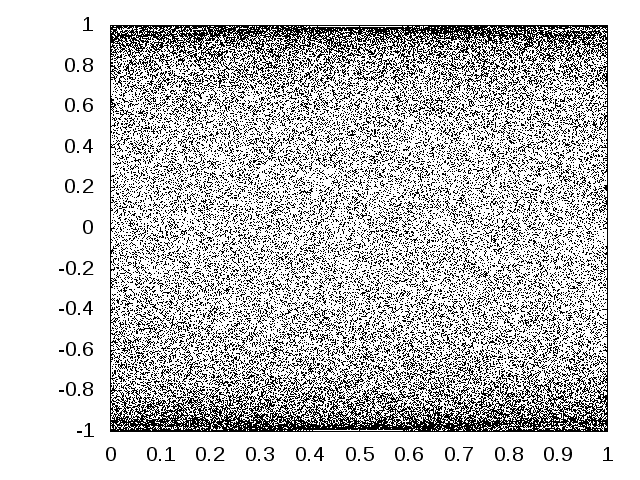
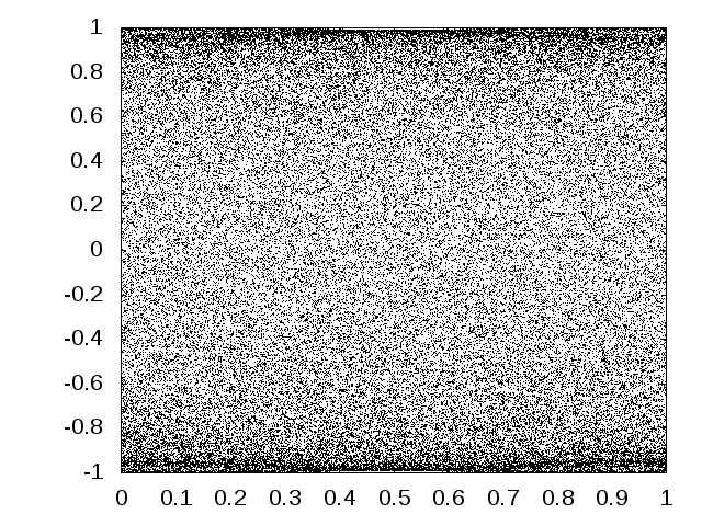
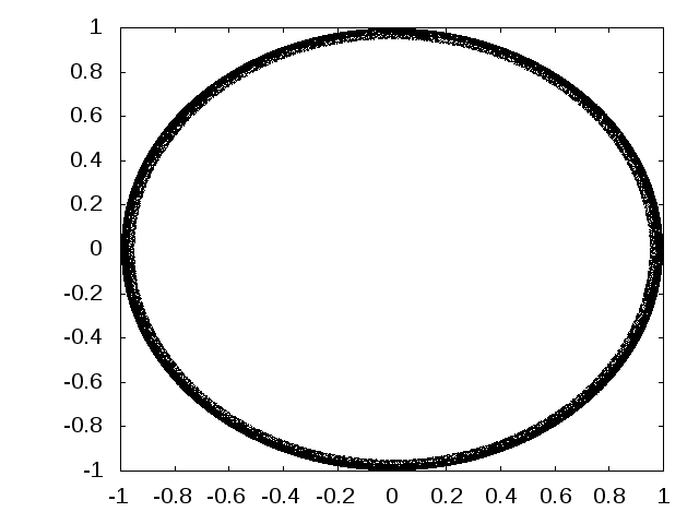
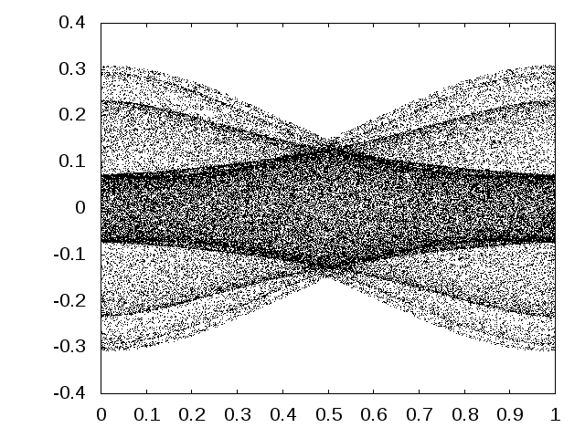
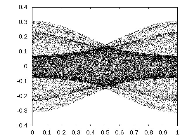
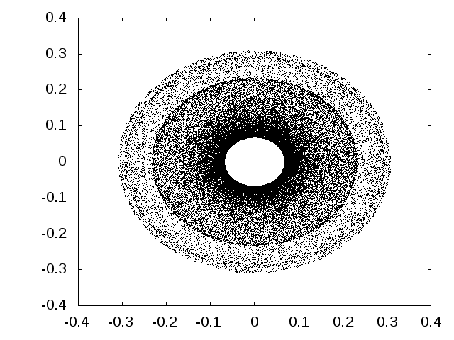
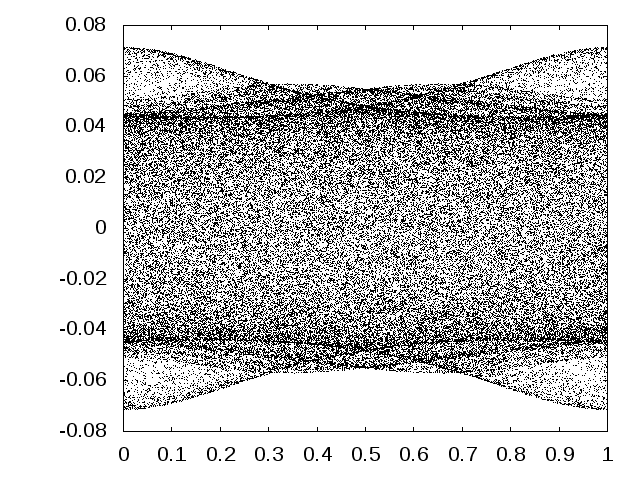
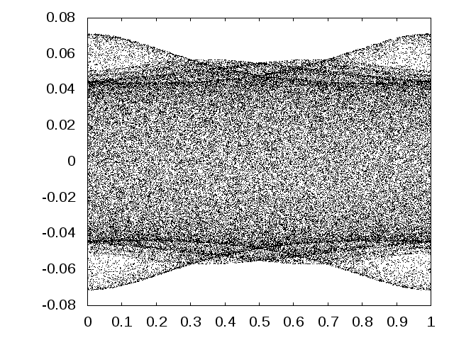
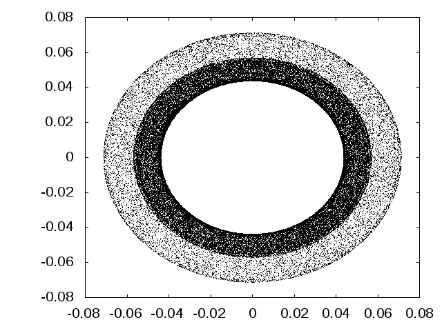
Figure 4: Several planar projections of the attractor of the map (30). Form left to right, and top to bottom we have the projections in the coordinates $(\omega,x_{0})$, $(\omega,y_{0})$, $(x_{0},y_{0})$, $(\omega,x_{2})$, $(\omega,y_{2})$, $(x_{2},y_{2})$, $(\omega,x_{4})$, $(\omega,y_{4})$ and $(x_{4},y_{4})$.

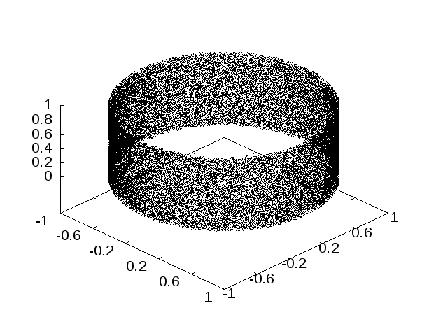
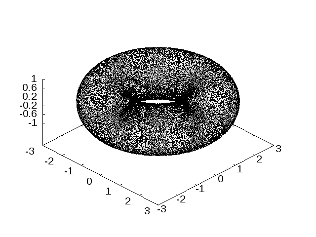
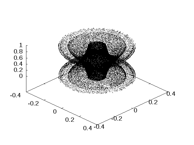
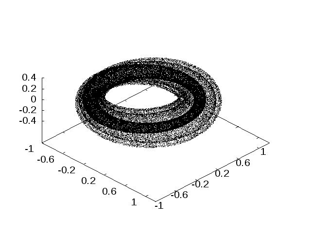
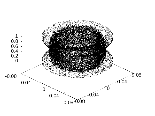
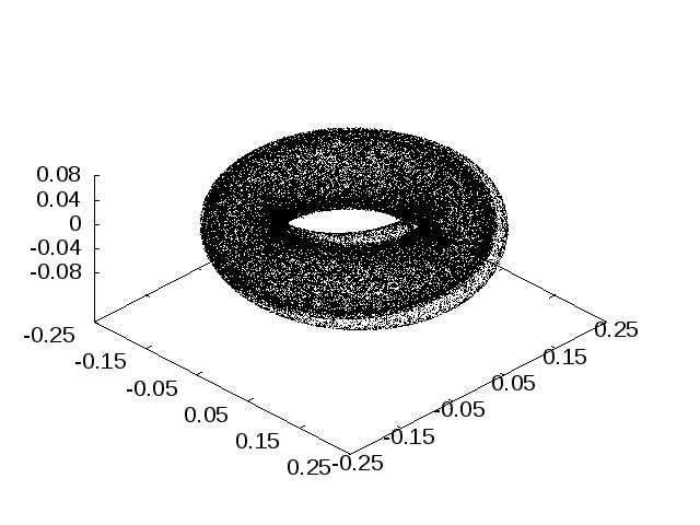
Figure 5: Several spatial projections of the attractor of the map (30). In the left hand side of the picture we have a plot (from top to bottom) of the projections in the coordinates $(\omega,x_{0},y_{0})$, $(\omega,x_{2},y_{2})$ and $(\omega,x_{4},y_{4})$. In the right hand side there are displayed the image of the left side projections taking a map that embeds the solid torus in $\mathbb{R}^{3}$ (see the text for more details).

We can use the discretization of $\mathcal{L}_{\omega}$ described in Appendix A to study numerically the maps $\tilde{L}_{1}$ and $L_{1}$. Let us focus first on the case concerning $\tilde{L}_{1}$. Given $v\in\mathcal{B}_{1}=\mathcal{RH}(\mathbb{W})\oplus\mathcal{RH}(\mathbb{W})$, consider the coordinates of $v=(x,y)$ given by this splitting. Following the discretization described in Appendix A each function $x\in\mathcal{RH}(\mathbb{W})$ can be approximated by the vector $(x_{0},x_{1},x_{2},...,x_{N})\in\mathbb{R}^{N+1}$ where $x_{i}$ is the $i$-th coefficient of the Taylor expansion for $x$ around $0$. This also holds for $y$, the second component of $v$. With this procedure each element $v$ in $\mathcal{B}_{1}$ can be approximated by a vector $(x_{0},x_{1},...,x_{N},y_{0},...,y_{N})$ in $\mathbb{R}^{2(N+1)}$.

Following the same argument we can approximate $\tilde{L}_{1}:\mathbb{T}\times\mathcal{B}_{1}\rightarrow\mathbb{T}\times\mathcal{B}_{1}$ by a map $\tilde{L}_{1}^{(N)}:\mathbb{T}\times\mathbb{R}^{2(N+1)}\rightarrow\mathbb{T}\times\mathbb{R}^{2(N+1)}$. We can use the discretized map $L_{1}^{(N)}$ to study the dynamics of $\tilde{L}_{1}$. Given an initial point $v_{0}=(x^{0},y^{0})\neq 0$, we have iterated the point by the map a certain transient $N_{1}$ and then we have plotted the following $N_{2}$ iterates. Figures 4 and 5 show different projections of the attracting set. The values taken for this discretization are $N=30$, $N_{1}=2000$ and $N_{2}=80000$. We have displayed the coordinates corresponding to the first even Taylor coefficients of the functions $x$ and $y$. The odd Taylor coefficients obtained were all equal to zero. This last observation suggest that the attractor is contained in the set of even functions (note that the subspace of $\mathcal{B}_{1}$ consisting of all the even functions is invariant by $\mathcal{L}_{\omega}$).

The same computations have been done for bigger values of $N$ and the results are the same. This indicates that the set obtained is stable with respect to the order of discretization, therefore it is reasonable to expect that it is close to the true attracting set of the original system.

Let us remark that we have not made explicit the initial values of $w_{0}$ and $v_{0}$ taken for the computations. Indeed, the results seem to be independent of these values. We have repeated this computation taking as initial value of $v_{0}$ all the elements of the canonical base of the discretized space $\mathbb{R}^{2(N+1)}$ and we have always obtained the same results. We have also repeated the computations for several values of $\omega_{0}$ obtaining always the same results.

Given a solid torus $\mathbb{T}\times\mathbb{D}_{\rho}$, with $\mathbb{D}_{\rho}$ the disk of radius $\rho$ in $\mathbb{C}$, we have that the map $f(\theta,x+iy)=(\cos(\theta)(x+K_{0}),\sin(\theta)(x+K_{0}),y)$ embeds this torus in $\mathbb{R}^{3}$, for any $K_{0}>\rho$. This embedding can be used for a better visualization of the spatial projections of the attracting set of the map (31). In the right hand side of figure 5 we have plotted the image by the embedding of the points on the left hand side. The concrete values of $K_{0}$ taken are (from above to below) $2$, $3/4$ and $3/20$.

The numerical approximation of the attractor displayed in figures 4 and 5 reveal the rotational symmetry of the attractor. This is the rotational symmetry described in section 3.1.

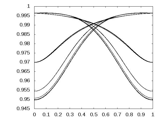
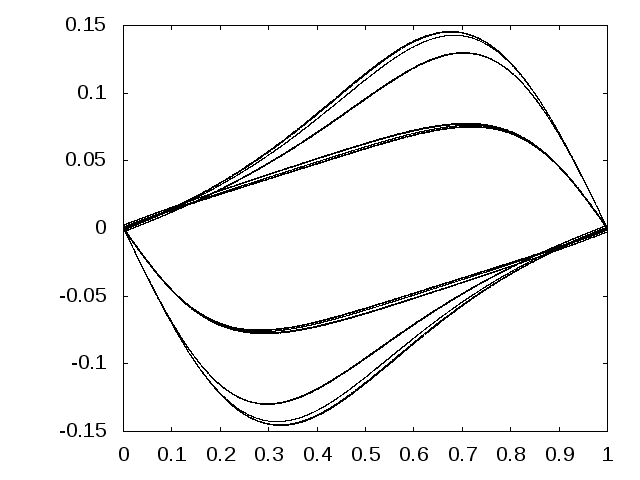
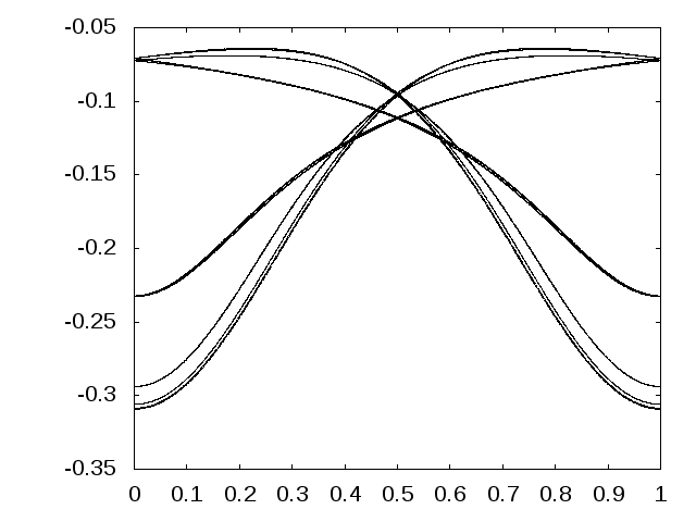
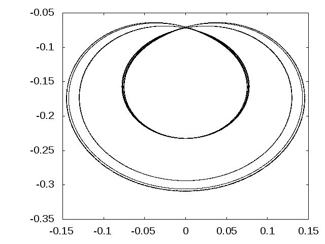
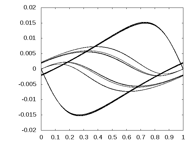
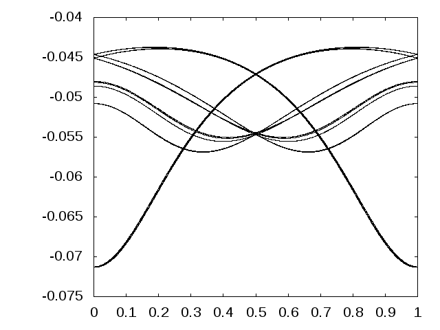
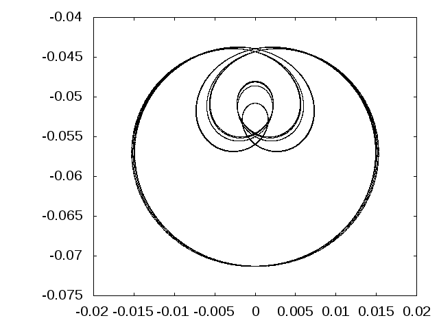
Figure 6: Several planar projections of the section of attractor of the map (31). Form left to right, and top to bottom we have the projections in the coordinates $(\omega,y_{0})$, $(\omega,x_{2})$, $(\omega,y_{2})$, $(x_{2},y_{2})$, $(\omega,x_{4})$, $(\omega,y_{4})$ and $(x_{4},y_{4})$.

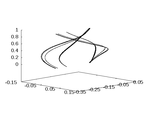
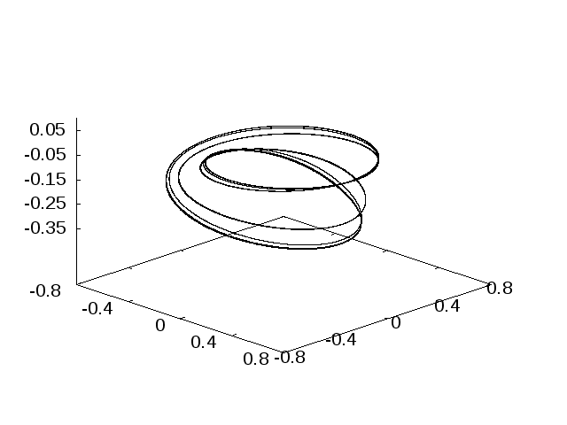
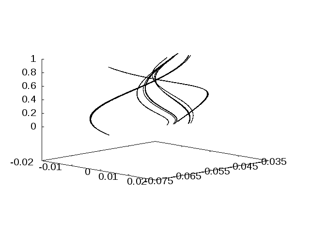
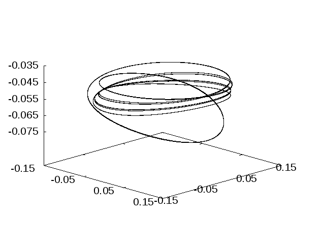
Figure 7: Several spatial projections of the intersection of the attractor of the map (31). The figures in the left correspond to the projection to the coordinates $(\omega,x_{2},y_{2})$ (top) and $(\omega,x_{4},y_{4})$ (bottom). In the right hand side there are displayed the image of the left side projections taking a map that embeds the solid torus in $\mathbb{R}^{3}$ (see the text for more details).

We can use the discretization described in Appendix A to approximate numerically the dynamics of $L_{1}$, as we have just done in the case of $\tilde{L}_{1}$. For the numerical simulation of the operator, we have taken $\theta_{0}=0$ and $x_{0}=0$. In this case the set $\mathcal{B}^{\prime}_{1}(0,0)$ is identified in $\mathbb{R}^{2(N+1)}$ with the half hyperplane

$$\{(x,y)\in\mathbb{R}^{2(N+1)}\thinspace|\thinspace x_{0}=0\text{ and }y_{0}>0\},$$

where $x_{0}$ and $y_{0}$ are respectively the first components of $x$ and $y$.

In figures 6 and 7 there are displayed different projections of the attracting set obtained iterating the map $L_{1}$. As before we have also considered the map $f(\theta,x+iy)=(\cos(\theta)(x+K_{0}),\sin(\theta)(x+K_{0}),y)$ which embeds the solid torus $\mathbb{T}\times\mathbb{D}_{\rho}$ in $\mathbb{R}^{3}$ for a better visualization of the set. This time the values of $K_{0}$ have been taken equal to $1/2$ (above) and $3/25$ (below).

Note that the different projections of the attracting set displayed in figure 6 keep a big resemblance with the plots of the dyadic solenoid displayed in figure 5 of [18]. Indeed we believe that the attractor is the inclusion of a dyadic solenoid in $\mathcal{B}_{1}^{\prime}$. For more details on the definition and the dynamics of the solenoid map see [2, 14, 18, 24]. To explain this fact, let us introduce a new conjecture, this time on the operator $L_{1}$.

Figure 8: Numerical approximation of the spectrum of $\mathcal{L}_{\omega}^{\prime}$ with respect to the parameter $\omega$. From left to right we have the real part, the imaginary part and the modulus of the first eight eigenvalues of $\mathcal{L}_{\omega}^{\prime}$ with respect to $\omega$.

Conjecture C.

There exist an open set $V\subset\mathcal{B}_{1}^{\prime}$ (independent of $\omega$) such that the second component of the map $L_{1}$ given by (31) is contractive (with the supremum norm) in the unit sphere and it maps the set $V$ into itself for any $\omega\in\mathbb{T}$. Additionally we will assume that the contraction is uniform for any $\omega\in\mathbb{T}$, in the sense that there exists a constant $0<\rho<1$ such that the Lipschitz constant associated to the second component of the map $L_{1}^{\prime}$ is upper bounded by $\rho$ for any $\omega\in\mathbb{T}$.

A good reason to think that conjecture C is true resides in the spectrum of the operator $\mathcal{L}^{\prime}_{\omega}$. In figure 8 we have a numerical approximation of this spectrum with respect to $\omega$ as a parameter. For this computation we have followed the same procedure that we used for the computation of the spectrum of $\mathcal{L}_{\omega}$, for details see Appendix A.

Looking at figure 8 we can observe that there exists a dominant eigenvalue (which is plotted in a dashed line) that does not cross the rest, which varies “nicely” with respect to $\omega$. Then for each value of $\omega$, the normalization of $\mathcal{L}^{\prime}_{\omega}$ is a contraction in the sphere, with the eigenvector associated to the dominant eigenvalue as a fixed point. This means that conjecture C is true “point-wise”, but this is not enough because the domain of contractivity might depend on $\omega$.

Let us justify now why conjecture C would explain the numerical results obtained for the attractor of $L_{1}$. Consider the set $\mathbb{T}\times V\subset\mathbb{T}\times\mathcal{B}^{\prime}_{1}(x_{0},\theta_{0})$. If the conjecture C is true, then we would have that the set $v$ invariant by the map $L_{1}$. More concretely we would have that the set would be expanded to the double of its length on the $\mathbb{T}$ direction and contracted in the $\mathcal{B}_{1}^{\prime}$ direction. Assume that this transformation is done in such a way that $L_{1}$ maps the set $\mathbb{T}\times V$ inside itself but without self intersections. When we consider the intersection of $L_{1}(\mathbb{T}\times V)$ with a set of the type $\{\gamma_{0}\}\times V$ (for some $\gamma_{0}\in T$) the section is conformed by two different sets without self intersections. The subsequent images by $L_{1}$ we would have (for each leaf $\{\gamma_{0}\}\times V$) the double of components than in the previous step, each of them strictly contracted in the $\mathcal{B}^{\prime}_{1}$ component and contained in the previous set. Note that the described process is completely analogous to the geometric construction of a dyadic solenoid, but this time contained inside the Banach space $\mathcal{B}^{\prime}_{1}$ instead of the solid torus. Therefore conjecture C would give an explanation to the numerical approximation of the attracting set of $L_{1}$ obtained before.

Consider $\{c_{1}(\alpha,\varepsilon)\}$ and $\{c_{2}(\beta,\varepsilon)\}$ two different families of two parametric maps satisfying hypotheses H1, H2’ and H3. Since the family of maps satisfy hypothesis H2’, we have that $\partial_{\varepsilon}c_{i}(\alpha^{*},0)$ belongs to $\mathcal{B}_{1}$ for $i=1,2$. Therefore the dynamics of $L$ (29) coincide with the dynamics of $L_{1}$ (31). Theorem 3.10 in [23] asserts the following.

Consider $\{c_{1}(\alpha,\varepsilon)\}$ and $\{c_{2}(\beta,\varepsilon)\}$ two different families of two parametric maps satisfying hypotheses H1 and H2’. Let $\alpha^{*}$ and $\beta^{*}$ be the parameter values where each family $c_{1}(\alpha,0)$ and $c_{2}(\beta,0)$ intersects $W^{s}(\mathcal{R},\Phi)$, the stable manifold of the fixed point of the renormalization operator. Let $\operatorname{Rot}(V)=\left\{v\in\mathcal{B}_{1}\thinspace|\thinspace t_{\gamma}(v)\in V\subset\mathcal{B}_{1}^{\prime}\text{ for some }\gamma\in\mathbb{T}\right\}$ where $V$ is the set given by conjecture C for some $\gamma\in\mathbb{T}$. If $\partial_{\varepsilon}c_{i}(\alpha^{*},0)$ belongs to $\operatorname{Rot}(V)$ for $i=1,2$ and the conjectures A, B and C are true, then (for any $\omega_{0}\in\Omega$) we have that

$$\frac{\alpha_{n}^{\prime}(\omega_{0},c_{1})}{\alpha_{n-1}^{\prime}(\omega_{0},c_{1})}\sim\frac{\alpha_{n}^{\prime}(\omega_{0},c_{2})}{\alpha_{n-1}^{\prime}(\omega_{0},c_{2})},$$ (33)

where $\alpha_{i}^{\prime}(\omega_{0},c_{i})$ are the reducibility loss directions associated to each family $c_{i}$ for the rotation number of the system equal to $\omega_{0}$.

3.4 Theoretical explanation to the second numerical observation

As before consider a two parametric family of maps $\{c(\alpha,\varepsilon)\}_{(\alpha,\varepsilon)\in A}$ satisfying hypothesis H1, H2’ and H3’ and let $\alpha^{\prime}_{n}(\omega,c)$ denote the slope of one of the curves of the reducibility loss bifurcation associated to the $2^{n}$ periodic invariant curve of the family. In theorem 3.13 of [23] we prove that the second numerical observation done in section 1.1 can be explained as a consequence of the universal behavior (33). One of the hypothesis to prove this requires $\alpha^{\prime}_{i}(\omega,c)/\alpha^{\prime}_{i}(2\omega,c)$ to be a bounded sequence.

The boundedness of this sequence can be obtained on its turn as a consequence of the following conjecture on the operator $\mathcal{L}_{\omega}$.

Conjecture D.

Consider $\mathcal{L}_{\omega}:\mathcal{RH}(\mathbb{W}_{\rho})\oplus\mathcal{RH}(\mathbb{W}_{\rho})\rightarrow\mathcal{RH}(\mathbb{W}_{\rho})\oplus\mathcal{RH}(\mathbb{W}_{\rho})$ the map given by (11) and $\omega_{0}\in\Omega$. Given $v_{0,1}$ and $v_{0,2}$ two vectors in $\mathcal{RH}(\mathbb{W}_{\rho})\oplus\mathcal{RH}(\mathbb{W}_{\rho})\setminus\{0\}$, consider the sequences

$$\begin{array}[]{rcll}\omega_{k}&=&2\omega_{k-1}&\text{ for }k=1,...,n-1.\\ \rule{0.0pt}{17.22217pt}v_{k,1}&=&\mathcal{L}_{\omega_{k-1}}\left(u_{k-1,1}\right)&\text{ for }k=1,...,n-1.\\ \rule{0.0pt}{17.22217pt}v_{k,2}&=&\mathcal{L}_{2\omega_{k-1}}\left(u_{k-1,2}\right)&\text{ for }k=1,...,n-1.\end{array}$$ (34)

Then, there exist constants $C_{1}$ and $C_{2}$ such that

$$C_{1}\frac{\|v_{0,2}\|}{\|v_{0,1}\|}\leq\frac{\|v_{n,2}\|}{\|v_{n,1}\|}\leq C_{2}\frac{\|v_{0,2}\|}{\|v_{0,1}\|}$$

for any $n\geq 0$.

Figure 9: We have $\frac{\|v_{0,1}\|}{\|v_{0,2}\|}\frac{\|v_{n,2}\|}{\|v_{n,1}\|}$ with respect to $n$, from $n=0$ to $n=20$ in the left and from $n=0$ to $n=2\times 10^{4}$ in the right.

This conjecture can be interpreted as a uniform growth condition on $\mathcal{L}_{\omega}$. To support this conjecture we have computed numerically the iterates (34), in order to estimate the growth of $\|v_{n,1}\|$ with respect to the growth of $\|v_{n,2}\|$. In figure 9 we have plotted the ratios $\frac{\|v_{0,1}\|}{\|v_{0,2}\|}\frac{\|v_{n,2}\|}{\|v_{n,1}\|}$ with respect to $n$ for the sequence (34) with $v_{0,1}=1$ and $v_{0,2}=1$. For other initial vectors we obtain the same behavior. This suggests that conjecture D is true.

Given $\{c(\alpha,\varepsilon)\}$ a two parametric maps satisfying hypotheses H1, H2’ and H3 let $\alpha^{*}$ be the parameter values for which the family $\{c(\alpha,0)\}_{(\alpha,0)\in A}$ intersects $W^{s}(\mathcal{R},\Phi)$. Let $\operatorname{Rot}(V)=\left\{v\in\mathcal{B}_{1}\thinspace|\thinspace t_{\gamma}(v)\in V\subset\mathcal{B}_{1}^{\prime}\text{ for some }\gamma\in\mathbb{T}\right\}$ where $V$ is the set given by conjecture C for some $\gamma\in\mathbb{T}$. Assume that $\partial_{\varepsilon}c(\alpha^{*},0)\in\operatorname{Rot}(V)$. In corollary 3.14 of [23] we prove that, for any $\omega_{0}\in\Omega$, then

$$\lim_{n\rightarrow\infty}\frac{\alpha_{n}^{\prime}(\omega_{0},c)}{\alpha_{n-1}^{\prime}(2\omega_{0},c)}$$ (35)

exists, which explains the second numerical observation of section 1.1.

3.5 Theoretical explanation to the third numerical observation

In sections 3.3 and 3.4 we focussed the discussion on the asymptotic behavior for families satisfying hypothesis H2’. The map considered in the third numerical observation of section 1.1 is an example of a map not satisfying H2’ for which equations (33) and (35) do not hold.

Let $\{c(\alpha,\varepsilon)\}_{(\alpha,\varepsilon)\in A}$ be a two parametric family of maps satisfying hypothesis H1, H2 and H3. Let $\alpha^{\prime}_{n}(\omega,c)$ denote slope of the reducibility loss bifurcation associated to the $2^{n}$ periodic invariant curve of the family. Finally consider $\omega_{0}$ a Diophantine rotation number for the family. Let $\alpha^{*}$ be the parameter value for which $\{c(\alpha,0)\}_{(\alpha,0)\in A}$ intersects $W^{s}(\Phi,\mathcal{R})$.

The main difference between the example considered in the third numerical observation of section 1.1 and the previous two is that

$$\partial_{\varepsilon}c(\alpha^{*},0)=v_{0,1}+v_{0,2}\text{ with }v_{0,i}\in\mathcal{B}_{i},\quad i=1,2,$$

where the spaces $\mathcal{B}_{i}$ are given by (10). More concretely, for the numerical example cited above we have considered

$$v_{0,1}=f_{1}(x)\cos(\theta),\quad v_{0,2}=\eta f_{2}(x)\cos(2\theta).$$ (36)

As this family depends on $\eta$, we denote by $c_{\eta}$ this concrete family. The parameter $\eta$ is considered in addition to the parameters $\alpha$ and $\varepsilon$ of the family. In other words, for each $\eta\geq 0$, $c_{\eta}$ is a two parametric family of maps.

Then one has that equation (28) still holds with $v_{n}=v_{n,1}+v_{n,2}$, with $v_{n,1}$ and $v_{n,2}$ the sequence given by (34) and $v_{0,1}$ and $v_{0,2}$ given by (36). In this case there is no universal behavior because the sequence $v_{n}$ lives in a bigger invariant space, where the renormalization operator is not contractive. On the other hand, the numerical computations in [21] suggest that the sequence $\alpha_{n}^{\prime}(\omega_{0},c_{\eta})/\alpha_{n-1}^{\prime}(\omega_{0},c_{\eta})$ (for $\eta>0$) is not asymptotically equivalent to $\alpha_{n}^{\prime}(\omega_{0},c_{0})/\alpha_{n-1}^{\prime}(\omega_{0},c_{0})$, but both sequences are $\eta$-close to each other. This can be explained as a consequence conjecture D where we conjecture uniform growth (in norm) of the sequences $v_{n,1}$ and $v_{n,2}$. For more details see theorem 3.20 in [23].

4 Applicability to the Forced Logistic Map

The theory exposed in sections 2 and 3 have been built as a response to the observations done in the study of the Forced Logistic Map (see [11, 21]). In this section we discuss the applicability of the quasi-periodic renormalization theory to the Forced Logistic Map. In the cited papers we considered two different version of the FLM, which correspond to the map (2) with either $h_{\alpha,\varepsilon}(\theta,x)=\alpha x(1-x)\cos(2\pi\theta)$ or $h_{\alpha,\varepsilon}(\theta,x)=\cos(2\pi\theta)$, where the parameters $(\alpha,\varepsilon)\in[0,4]\times[0,1]$. Notice that these two forms of the FLM do not satisfy the requirements of the theory developed in the previous sections because the family of maps does not belong to $\mathcal{B}$.

This problem can be easily solved as follows. For $\alpha>2$ we can consider the affine change of variables given by $y=ax+b$, with $a=\frac{4}{\alpha-2}$ and $b=-\frac{2}{\alpha-2}$. If we apply this change of variables to the family (2) when $h_{\alpha,\varepsilon}(\theta,x)=\alpha x(1-x)\cos(2\pi\theta)$ we obtain the following family,

$$\left.\begin{array}[]{rcl}\bar{\theta}&=&\theta+\omega,\\ \bar{y}&=&\alpha\displaystyle\left(\frac{\alpha}{\alpha-2}-\frac{\alpha(\alpha-2)}{4}y^{2}\right)(1+\varepsilon\cos(2\pi\theta))-\frac{2}{\alpha-2}.\end{array}\right\}$$ (37)

If we apply the same change of variables when $h_{\alpha,\varepsilon}(\theta,x)=\cos(2\pi\theta)$ we obtain this other family

$$\left.\begin{array}[]{rcl}\bar{\theta}&=&\theta+\omega,\\ \bar{y}&=&\displaystyle 1-\frac{\alpha(\alpha-2)}{4}y^{2}+\frac{4\varepsilon}{\alpha-2}\cos(2\pi\theta).\end{array}\right\}$$ (38)

Although the change of variables considered depends on the parameter $\alpha$, the parameter space of the maps (37) and (38) is the same as the parameter space of the map (2) (for the corresponding value of $h$). Then any conclusion drawn on the parameter space of the map (37) (respectively (38)) extends automatically to the parameter space of (2).

With this new set up, we have that both families of maps belong to $\mathcal{B}$ for $\alpha\in(2,4)$ and $\varepsilon$ small enough. One should check that the FLM satisfies hypotheses H1 and H2’. To check H1 one should check that the one dimensional Logistic Map intersects transversally $W^{s}(\Phi,\mathcal{R})$ the stable manifold of the renormalization operator. This is an implicit assumption when one uses the renormalization operator to explain the universality observed for the Logistic Map. The only proof (to our knowledge) of this fact is the one given by Lyubich (theorem 4.11 of [17]). This proof is done in the space of quadratic-like germs, which is a smaller space than the one considered here. Hypothesis H2’ is trivial to check for the maps (37) and (38)).

On the other hand, note that theorem 3.8 in [22] not only gives the existence of reducibility loss bifurcations, but it also gives an explicit expression of its slopes in term of the renormalization operator (the ones given by formulas (18) and (19)). Actually we have given even a more explicit formula in corollary 3.13 in [22]. We used these formulas to compute the reducibility directions $\alpha_{n}^{\prime}(\omega)$ of the Forced Logistic Map (37).

The initial values $\alpha_{n}$ have been computed numerically, by means of a Newton method applied to their invariance equation. Differentiating on formula (37) (respectively (38)) it is easy to write the values of $f^{(n)}_{0},u^{(n)}_{0}$ and $v^{(n)}_{0}$ in terms of $\alpha_{n}$. Then using the discretization of the operator done in Appendix A, we can compute numerically the iterates $f^{(n)}_{k},u^{(n)}_{k}$ and $v^{(n)}_{k}$, for $k=1,...,n-1$. Once we have these functions, we can evaluate them to compute the values of $\alpha^{\prime}_{n}(\omega)$ given by formula ($48$) of [22].

n	$\alpha^{\prime}_{n}(\omega)$	$\bar{\epsilon}_{a}$	$\bar{\epsilon}_{r}$
1	-5.832915e+00	1.986668e-15	3.405962e-16
2	-8.494260e+00	1.155106e-13	1.359866e-14
3	-1.635128e+01	1.265556e-14	7.739800e-16
4	-1.125246e+01	3.995769e-14	3.551018e-15
5	-1.224333e+01	1.235427e-12	1.009061e-13
6	-1.807969e+01	8.989082e-12	4.971921e-13
7	-3.473523e+01	8.087996e-11	2.328470e-12
8	-2.958331e+01	2.204433e-10	7.451609e-12
9	-4.156946e+01	1.293339e-09	3.111273e-11
10	-7.896550e+01	3.847537e-08	4.872428e-10
11	-7.450073e+01	7.779131e-08	1.044168e-09

Table 2: Values of $\alpha^{\prime}_{n}(\omega)$ for the FLM map (37) and $\omega=\frac{\sqrt{5}}{2}$. The values $\bar{\varepsilon}_{a}$ and $\bar{\varepsilon}_{r}$ correspond to the discrepancy with the estimates of [21] in absolute and relative terms.

We have used this procedure to compute the values of $\alpha^{\prime}_{n}(\omega)$ for the map (37) (consequently also for the map (2) with $h_{\alpha,\varepsilon}(\theta,x)=\alpha x(1-x)\cos(2\pi\theta)$) and $\omega_{0}=\frac{\sqrt{5}-1}{2}$. The results are shown in table 2. The values $\alpha^{\prime}_{n}(\omega)$ have been also computed in [21] via a completely different procedure, based on a continuation method with extended precision. More concretely these values are displayed in table $2$ of the cited paper. The third and fourth columns of table 2 display the discrepancies between both computation, in absolute ($\bar{\epsilon}_{a}$) and relative ($\bar{\epsilon}_{r}$) terms. This experiment has been repeated for other values of $\omega$ and also for the map (38). In all cases we obtained that the slopes computed with both methods are the same up to similar accuracies to the ones displayed in table 2.

This supports the correctness of both computations and at the same time the conjecture A, which has been assumed to be true to derive the formula used for this estimation.

Appendix A Numerical computation of the spectrum of $\mathcal{L}_{\omega}$

In this appendix we present the numerical method that we used to discretize $\mathcal{L}_{\omega}$ and to study its spectrum numerically. Our method is a slight modification of the one introduced by Lanford in [15] (see also [16]).

Let $\mathbb{D}(z_{0},\rho)$ be the complex disc centered on $z_{0}$ with radius $\rho$. Consider $\mathcal{RH}(\mathbb{D}(z_{0},\rho))$ the space of real analytic functions such that they are holomorphic on $\mathbb{D}(z_{0},\rho)$ and continuous on it closure. Given a function $f\in\mathcal{RH}(\mathbb{D}(z_{0},\rho))$, we can consider the following modified Taylor expansion of $f$ around $z_{0}$,

$$f(z)=\sum_{k=0}^{\infty}f_{i}\left(\frac{z-z_{0}}{\rho}\right)^{i}.$$ (39)

The truncation of a Taylor series at order $N$ induces a projection defined as

$$\begin{array}[]{rccc}p_{(N)}:&\mathcal{RH}(\mathbb{D}_{\rho})&\rightarrow&\mathbb{R}^{N+1}\\ &f&\mapsto&(f_{0},f_{1},\dots,f_{N}),\end{array}$$

On the other hand we have its pseudo-inverse by the left

$$\begin{array}[]{rccc}i_{(N)}:&\mathbb{R}^{N+1}&\rightarrow&\mathcal{RH}(\mathbb{D}_{\rho})\\ &(f_{0},f_{1},\dots,f_{N})&\mapsto&\displaystyle\sum_{k=0}^{N}f_{i}\left(\frac{z-z_{0}}{\rho}\right)^{i},\end{array}$$

in the sense that $i_{(N)}\circ p_{(N)}$ is the identity on $\mathbb{R}^{N+1}$. Note also that both maps are linear.

Given a map $T:\mathcal{RH}(\mathbb{D}(z_{0},\rho))\rightarrow\mathcal{RH}(\mathbb{D}(z_{0},\rho))$, we can approximate it by its discretization $T^{(N)}:\mathbb{R}^{N+1}\rightarrow\mathbb{R}^{N+1}$ defined as $T^{(N)}:=p_{(N)}\circ T\circ i_{(N)}$. More concretely if $T$ is a linear bounded operator, we can compute the eigenvalues of the operator $T^{(N)}$ in order to study the spectrum of $T$. In general the eigenvalues of $T^{(N)}$ might have nothing to do with the spectrum of $T$. For example an infinite-dimensional operator does not need to have eigenvalues, but a finite-dimensional one will always have the same number of eigenvalues (counted with multiplicity) as the dimension of the space. For this reason will do some numerical test on the results obtained with this discretization.

At this point consider the map $\mathcal{L}_{\omega}:\mathcal{RH}(\mathbb{W})\oplus\mathcal{RH}(\mathbb{W})\rightarrow\mathcal{RH}(\mathbb{W})\oplus\mathcal{RH}(\mathbb{W})$ defined by equation (11). If we set $\mathbb{W}=\mathbb{D}(z_{0},\rho)$ we can use the method described above in each component of $\mathcal{RH}(\mathbb{W})\oplus\mathcal{RH}(\mathbb{W})$ to discretize $\mathcal{L}_{\omega}$ and approximate it by a map $\mathcal{L}_{\omega}^{(N)}:\mathbb{R}^{2(N+1)}\rightarrow\mathbb{R}^{2(N+1)}$. Concretely in our computation we have taken $z_{0}=\frac{1}{5}$ and $\rho=\frac{3}{2}$. In figure 2 we include graphical evidence that the set $\mathbb{W}=\mathbb{D}\left(\frac{1}{5},\frac{3}{2}\right)$ satisfies H0, in section 2.1 can be found more details about this.

$i$	$\lambda_{i}$	$i$	$\lambda_{i}$
1	+7.8412640 +1.5617754$i$	13	-0.0637772 +0.0000000$i$
2	+7.8412640 -1.5617754$i$	14	-0.0637772 -0.0000000$i$
3	-2.5029079 +0.0000000$i$	15	+0.0430641 +0.0435724$i$
4	-2.5029079 +0.0000000$i$	16	+0.0430641 -0.0435724$i$
5	+0.5114250 +0.1942111$i$	17	-0.0178305 +0.0165287$i$
6	+0.5114250 -0.1942111$i$	18	-0.0178305 -0.0165287$i$
7	+0.4881230 +0.4930710$i$	19	-0.0101807 +0.0000000$i$
8	+0.4881230 -0.4930710$i$	20	-0.0101807 -0.0000000$i$
9	-0.3995353 +0.0000000$i$	21	+0.0075181 +0.0069602$i$
10	-0.3995353 +0.0000000$i$	22	+0.0075181 -0.0069602$i$
11	-0.0982849 +0.0869398$i$	23	-0.0029419 +0.0027336$i$
12	-0.0982849 -0.0869398$i$	24	-0.0029419 -0.0027336$i$

Table 3: The first twenty four eigenvalues of $\mathcal{L}_{\omega}^{(N)}$, for $\omega=\frac{1-\sqrt{5}}{2}$. For the computation $N$ has been taken equal to 100.

In table 3 we have the first $24$ eigenvalues of $\mathcal{L}_{\omega}^{(N)}$ for $N=100$ and $\omega=\frac{\sqrt{5}-1}{2}$. The eigenvalues have been sorted by their modulus, from bigger to smaller. Note that the eigenvalues of the discretized operator also satisfy the properties given in section 2.1. To justify the validity of these eigenvalues we have done the following numerical tests.

Figure 10: Estimation of the errors and the radii of convergence of the first twenty-four eigenvalues of $\mathcal{L}_{\omega}$ for $\omega=\frac{\sqrt{5}-1}{2}$ with respect to the order of the discretization. See the text for more details.

Consider that we have a real eigenvalue of multiplicity two, or a pair of complex eigenvalues which is persistent for different values of $N$ (the order of the discretization). The first test done to the eigenvalues is to check if the distance between the associated eigenvectors decreases when $N$ is increased. In the left part of figure 10 we have the distance between the eigenvectors associated to the same eigenvalue of the operators $\mathcal{L}^{(N)}_{\omega}$ and $\mathcal{L}^{(110)}_{\omega}$ as a graph of $N$, with $N$ varying from $40$ to $100$. We have plotted this distance for the first twenty-four eigenvalues. To compute the distance between eigenvectors we have estimated the supremum norm of the difference between the real function represented by each of the vectors, in other words we have computed $\|i^{(N)}(v^{(N)})-i^{(110)}(v^{(110)})\|_{\infty}$ in the interval $(z_{0}-\rho,z_{0}+\rho)=\mathbb{W}\cap\mathbb{R}$.

Note that, since the distance goes to zero this indicates that the eigenvectors, namely $v^{(N)}$, converge to a limit $v^{*}$. One should expect these eigenvalues to be in the spectrum of $\mathcal{L}_{\omega}$, but nothing ensures that $v^{*}$ belongs to the domain of $\mathcal{L}_{\omega}$. We have done a second test on the reliability of the approximated eigenvectors, where we check this condition.

Let us remark that with the numerical computations done so far, we have only checked that the eigenvectors as elements of $\mathcal{RH}(\mathbb{D}(z_{0},\rho))\oplus\mathcal{RH}(\mathbb{D}(z_{0},\rho))$ to converge in the segment $(z_{0}-\rho,z_{0}+\rho)\subset\mathbb{R}$ instead of checking the convergence in the whole set $\mathbb{D}(z_{0},\rho)$. Let us give evidences that approximate eigenvectors obtained with our computations have a domain of analicity containing $\mathbb{D}(z_{0},\rho)$.

Consider that we have a function $f$ holomorphic in a domain of the complex plane containing $\mathbb{D}(z_{0},\rho)$. If the we consider the expansion of $f$ given by equation (39), we have that $r$ the radius of convergence of the series around $z_{0}$ is given as

$$r=\frac{\rho}{\limsup_{n\rightarrow\infty}\sqrt[n]{|f_{n}|}}.$$

With the discretization considered here we have an approximation of the terms $f_{n}$, hence these can be used to compute a numerical estimation of $r$.

Consider $v$ an eigenvector of the operator $\mathcal{L}_{\omega}$. We have that $v=(v_{1},v_{2})\in\mathcal{RH}(\mathbb{W})\oplus\mathcal{RH}(\mathbb{W})$. Given $v_{1}^{(N)}=(v_{1}^{(N)},v_{2}^{(N)})$ a numerical approximation of the eigenvector, we can use the procedure described above to estimate the radius of convergence of each $v_{1}$ and $v_{2}$. We have done this for the eigenvectors associated to each of the first twenty-four eigenvalues of $\mathcal{L}_{\omega}$ with $\omega=\frac{\sqrt{5}-1}{2}$ (keeping only the smaller of the two radius obtained). The results are displayed on the right part of figure 10, where the estimated radius has been plotted with respect to $N$, the order of the discretization. Note that the estimations give a radius bigger than $\rho=\frac{3}{2}$, which indicates that the eigenvectors are analytic in $\mathbb{D}(z_{0},\rho)$, and continuous on its closure, for $z_{0}=\frac{1}{5}$ and $\rho=\frac{3}{2}$.

Figure 11: Estimation of the distance between eigenvectors with the same eigenvalue (left) and estimation of the radios of convergence (right) of the first twenty-four eigenvalues of $\mathcal{L}_{\omega}$ with respect to $\omega$. See the text for more details.

Up to this point, we have considered $\omega$ fixed to $\frac{\sqrt{5}-1}{2}$, but the same computations can be done to study the spectrum of $\mathcal{L}_{\omega}$ with respect to the parameter $\omega$. In figure 3 of section 2.1 we have plotted the first twenty-four eigenvalues of the map with respect to $\omega$. The set $\mathbb{T}$ has been discretized in a equispaced grid of $1280$ points. Recall that the operator $\mathcal{L}_{\omega}$ depends analytically on $\omega$ (proposition 2.20 in [22]), therefore the spectrum also does (as long as the eigenvalues do not collide, see theorems III-6.17 and VII-1.7 in [13]). The numerical results agree with this analytic dependence.

For this computation we have also made the same test as before to the eigenvalues. The results of these tests are shown in figure 11. To estimate the convergence of the eigenvectors we have compared the eigenspaces of the eigenvalues of $\mathcal{L}_{\omega}^{(90)}$ with the eigenspaces associated to $\mathcal{L}_{\omega}^{(100)}$ for each value of $\omega$ in the cited grid of points on $\mathbb{T}$. The estimation of the radius of convergence has been also done with respect to $\omega$ for $N=90$. We have plotted the estimated error and convergence radius for the first twenty-four eigenvalues in the same figure. Both result indicate that the eigenvalues obtained are reliable.

References

- [1] K. Bjerklöv. SNA’s in the quasi-periodic quadratic family. Comm. Math. Phys., 286(1):137–161, 2009.
- [2] H. W. Broer and F. Takens. Dynamical systems and chaos, volume 172 of Applied Mathematical Sciences. Springer, New York, 2011.
- [3] W. de Melo and S. van Strien. One-dimensional dynamics, volume 25 of Ergebnisse der Mathematik und ihrer Grenzgebiete (3) [Results in Mathematics and Related Areas (3)]. Springer-Verlag, Berlin, 1993.
- [4] J.-P. Eckmann and P. Wittwer. A complete proof of the Feigenbaum conjectures. J. Statist. Phys., 46(3-4):455–475, 1987.
- [5] M. J. Feigenbaum. Quantitative universality for a class of nonlinear transformations. J. Statist. Phys., 19(1):25–52, 1978.
- [6] M. J. Feigenbaum. The universal metric properties of nonlinear transformations. J. Statist. Phys., 21(6):669–706, 1979.
- [7] U. Feudel, S. Kuznetsov, and A. Pikovsky. Strange nonchaotic attractors, volume 56 of World Scientific Series on Nonlinear Science. Series A: Monographs and Treatises. World Scientific Publishing Co. Pte. Ltd., Hackensack, NJ, 2006. Dynamics between order and chaos in quasiperiodically forced systems.
- [8] J. Figueras and A. Haro. Computer assisted proofs of the existence of fiberwise hyperbolic invariant tori in skew products over rotations. To appear, 2010.
- [9] J. F. Heagy and S. M. Hammel. The birth of strange nonchaotic attractors. Phys. D, 70(1-2):140–153, 1994.
- [10] T. H. Jaeger. Quasiperiodically forced interval maps with negative schwarzian derivative. Nonlinearity, 16(4):1239–1255, 2003.
- [11] A. Jorba, P. Rabassa, and J.C. Tatjer. Period doubling and reducibility in the quasi-periodically forced logistic map. Preprint available at http://arxiv.org, 2011.
- [12] A. Jorba and J. C. Tatjer. A mechanism for the fractalization of invariant curves in quasi-periodically forced 1-D maps. Discrete Contin. Dyn. Syst. Ser. B, 10(2-3):537–567, 2008.
- [13] T. Kato. Perturbation Theory for Linear Operators. Springer Verlag, 1966.
- [14] A. Katok and B. Hasselblatt. Introduction to the Modern Theory of Dynamical Systems. Cambridge University Press, 1996.
- [15] O. E. Lanford, III. A computer-assisted proof of the Feigenbaum conjectures. Bull. Amer. Math. Soc. (N.S.), 6(3):427–434, 1982.
- [16] O. E. Lanford, III. Computer assisted proofs. In Computational methods in field theory (Schladming, 1992), volume 409 of Lecture Notes in Phys., pages 43–58. Springer, Berlin, 1992.
- [17] M. Lyubich. Feigenbaum-Coullet-Tresser universality and Milnor’s hairiness conjecture. Ann. of Math. (2), 149(2):319–420, 1999.
- [18] J. Milnor. On the concept of attractor. Comm. Math. Phys., 99(2):177–195, 1985.
- [19] A. Prasad, V. Mehra, and R. Ramaskrishna. Strange nonchaotic attractors in the quasiperiodically forced logistic map. Phys. Rev. E, 57(2):1576–1584, 1998.
- [20] P. Rabassa. Contribution to the study of perturbations of low dimensional maps. PhD thesis, Universitat de Barcelona, 2010.
- [21] P. Rabassa, A. Jorba, and J.C. Tatjer. Numerical evidences of universality and self-similarity in the forced logistic map. Preprint available at http://arxiv.org, 2011.
- [22] P. Rabassa, A. Jorba, and J.C. Tatjer. Towards a renormalization theory for quasi-periodically forced one dimensional maps I. Existence of reducibily loss bifurcations. Preprint available at http://arxiv.org, 2011.
- [23] P. Rabassa, A. Jorba, and J.C. Tatjer. Towards a renormalization theory for quasi-periodically forced one dimensional maps II. Asymptotic behavior of reducibility loss bifurcations. Preprint available at http://arxiv.org, 2011.
- [24] S. Smale. Differentiable dynamical systems. Bull. Amer. Math. Soc., 73:747–817, 1967.
- [25] D. Sullivan. Bounds, quadratic differentials, and renormalization conjectures. In American Mathematical Society centennial publications,Vol. II (Providence, RI, 1988), pages 417–466. Amer. Math. Soc., Providence, RI, 1992.
- [26] C. Tresser and P. Coullet. Itérations d’endomorphismes et groupe de renormalisation. C. R. Acad. Sci. Paris Sér. A-B, 287(7):A577–A580, 1978.