Finding D-optimal designs by randomised decomposition and switching

Abstract

A square $\{+1,-1\}$-matrix of order $n$ with maximal determinant is called a saturated D-optimal design. We consider some cases of saturated D-optimal designs where $n>2$, $n\not\equiv 0\bmod 4$, so the Hadamard bound is not attainable, but bounds due to Barba or Ehlich and Wojtas may be attainable. If $R$ is a matrix with maximal (or conjectured maximal) determinant, then $G=RR^{T}$ is the corresponding Gram matrix. For the cases that we consider, maximal or conjectured maximal Gram matrices are known. We show how to generate many Hadamard equivalence classes of solutions from a given Gram matrix $G$, using a randomised decomposition algorithm and row/column switching. In particular, we consider orders $26$, $27$ and $33$, and obtain new saturated D-optimal designs (for order $26$) and new conjectured saturated D-optimal designs (for orders $27$ and $33$).

1 Introduction

The Hadamard maximal determinant (maxdet) problem is to find the maximum determinant $D(n)$ of a square $\{+1,-1\}$-matrix of given order $n$. Such a matrix $A$ with maximal $|\det(A)|$ is called a saturated D-optimal design of order $n$. We are only concerned with the absolute value of the determinant, as the sign may be changed by a row or column interchange.

Hadamard [9] showed that $D(n)\leq n^{n/2}$, and this bound is attainable for $n>2$ only if $n\equiv 0\bmod 4$. The “Hadamard conjecture” (due to Paley [20]) is that Hadamard’s bound is attainable for all $n\equiv 0\bmod 4$. In this paper we are concerned with “non-Hadamard” cases $n>2$, $n\not\equiv 0\bmod 4$. For such orders the Hadamard bound is not attainable, but other upper bounds due to Barba [1], Ehlich [7, 8] and Wojtas [26] may be attainable. For lower bounds on $D(n)$, see Brent and Osborn [4], and the references given there.

We say that two $\{+1,-1\}$ matrices $A$ and $B$ are Hadamard-equivalent (abbreviated H-equivalent) if $B$ can be obtained from $A$ by a signed permutation of rows and/or columns. If $A$ is H-equivalent to $B$ or to $B^{T}$ then we say that $A$ and $B$ are extended Hadamard-equivalent (abbreviated HT-equivalent). Note that, if $A$ is HT-equivalent to $B$, then $|\det(A)|=|\det(B)|$.

If $A$ is H-equivalent to $A^{T}$ then we say that $A$ is self-dual. We say that a Hadamard equivalence class is self-dual if the class contains a self-dual matrix (equivalently, if the duals of all matrices in the class are also in the class).

If we know (or conjecture) $D(n)$, it is of interest to find all (or most) Hadamard equivalence classes of $\{+1,-1\}$ matrices with determinant $\pm D(n)$. In this paper we consider the orders $26$, $27$ and $33$; similar methods can be used for certain other orders.

In §2 we consider the randomised decomposition of (candidate) Gram matrices. Then, in §3, we show how one solution can often be used to generate other, generally not Hadamard equivalent, solutions via switching. The graph of Hadamard equivalence classes induced by switching is defined in §3. We conclude with some new results for the orders $26$, $27$ and $33$ in §§4–6.

Upper bounds

A bound which holds for all odd orders, and which is known to be sharp for an infinite sequence of orders $\equiv 1\pmod{4}$, is

$$D(n)\leq(2n-1)^{1/2}(n-1)^{(n-1)/2},$$ (1)

due independently to Barba [1] and Ehlich [7]. We call it the Barba bound. Brouwer [5] showed that the Barba bound (1) is sharp if $n=q^{2}+(q+1)^{2}$ for $q$ an odd prime power. The bound is also sharp in some other cases, e.g. $q=2$ and $q=4$. It is not achievable unless $n$ is the sum of two consecutive squares.

An upper bound due to Ehlich [8] applies only in the case $n\equiv 3\pmod{4}$. We refer to [3, 8, 18, 19] for details of this bound, which is rather complicated. The Ehlich bound is not known to be sharp for any order $n>3$.

Another bound,

$$D(n)\leq(2n-2)(n-2)^{(n-2)/2},$$ (2)

due to Ehlich [7] and Wojtas [26], applies in the case $n\equiv 2\pmod{4}$. It is known to be sharp in the following cases: (A) $n=2(q^{2}+(q+1)^{2})$, where $q$ is an odd prime power (see Whiteman [25]); and (B) $n=2(q^{2}+q+1)$, where $q$ is any (even or odd) prime power [22, 12].

Gram matrices

If $R$ is a given square matrix then the symmetric matrix $G=RR^{T}$ is called the Gram matrix of $R$. We may also consider the dual Gram matrix $H=R^{T}R$. Since $\det(G)=\det(R)^{2}$, the bounds mentioned above on $\det(R)$ are equivalent to bounds on $\det(G)$. Indeed, this observation explains the form of the bounds. For example, the Barba bound corresponds to a matrix $G=(g_{i,j})$ given by $g_{i,j}=n$ if $i=j$ and $g_{i,j}=1$ if $i\neq j$. It is easy to show via a well-known rank-1 update formula that $\det(G)=(2n-1)(n-1)^{n-1}$.

Given a symmetric matrix $G$ with suitable determinant, we say $G$ is a candidate Gram matrix. It is the Gram matrix of a $\{+1,-1\}$ matrix if and only if it decomposes into a product of the form $G=RR^{T}$, where $R$ is a square $\{+1,-1\}$ matrix.

2 Decomposition of candidate Gram matrices

Suppose that a (candidate) Gram matrix $G$ of order $n$ is known. We want to find one or more $\{+1,-1\}$ matrices $R$ such that $G=RR^{T}$. Let the rows of $R$ be $r_{1}^{T},\ldots,r_{n}^{T}$. Then

$$r_{i}^{T}r_{j}=g_{i,j},\;1\leq i,j\leq n.$$

If we already know the first $k$ rows, then we get $k$ single-Gram constraints involving row $k+1$:

$$r_{i}^{T}r_{k+1}=g_{i,k+1}\;{\rm for}\;1\leq i\leq k.$$

These are linear constraints in the unknowns $r_{k+1}$. We may be able to find one or more solutions for row $k+1$ satisfying the single-Gram constraints, or there may be no solutions, in which case we have to backtrack.

Our algorithm is described in [3, §4], so we omit the details here. We merely note that it is possible to take advantage of various symmetries to reduce the size of the search space, and that it is possible to prune the search using gram-pair constraints of the form $G^{j+1}=RH^{j}R^{T}$ ($j>0$) if we know the dual Gram matrix $H=R^{T}R$. In the cases considered below, there is (up to signed permutations) only one candidate Gram matrix with the required determinant, so there is no loss of generality in assuming that $G=H$.

The search can be regarded as searching a (large) tree with (at most) $n$ levels, where each level corresponds to a row of $R$. A deterministic search typically searches the tree in depth-first fashion – at each node, recursively search the subtrees defined by the children of that node. The aim is to find one or more leaves at the $n$-th level of the tree, since these leaves correspond to complete solutions $R$.

Deterministic, depth-first search may take a long time searching fruitlessly for solutions in subtrees where no solutions exist. When $G$ is decomposable, but difficult to decompose using a deterministic search, we may be able to do better with a randomised search.

In the randomised search, at each node we randomly choose a small number of children and recursively search the subtrees defined by these children. A good choice of the average number of children chosen per node, say $\mu$, can be determined experimentally. Too small a value makes it unlikely that a solution will be found; too large a value makes the search take too long. We found empirically that $\mu\approx 1.3$ works well in the cases considered below. Thus, at each node traversed in the search we choose one child (if there are any) and, with probability about $\mu-1\approx 0.3$, also choose a second child (if there is one), then recursively search the subtrees defined by the selected children.

For example, in the case $n=27$, there is a known Gram matrix $G$, due to Tamura [23], which decomposes into $RR^{T}$, giving a $\{+1,-1\}$ matrix $R$ of determinant $546\times 6^{11}\times 2^{26}$. This determinant is conjectured to be maximal.

A deterministic search fails to decompose Tamura’s $G$ in $24$ hours (exploring over $10^{8}$ nodes but reaching only depth $17$ in the search tree). The tree size is probably greater than $4\times 10^{9}$.

On the other hand, our randomised search routinely finds a decomposition of $G$ in about $90$ seconds. In this way we have found many different H-classes of solutions. Further details are given in §5.

Nonuniformity of sampling

Unfortunately, the randomised search strategy described above does not guarantee that the set of H-classes of solutions (or the set of all $\{+1,-1\}$ matrices of the given order and determinant) is sampled uniformly. There are two reasons for lack of uniformity. First, the tree-generation algorithm introduces non-uniformity by taking advantage of symmetries to reduce the size of the tree. Second, the number of matrices in a class is inversely proportional to the order of the automorphism group of the class, so even if all the $\{+1,-1\}$ matrices were sampled uniformly, the H-classes would not necessarily be sampled uniformly.

3 Switching

Switching is an operation on square $\{+1,-1\}$ matrices which preserves the absolute value of the determinant but does not generally preserve Hadamard equivalence or extended Hadamard equivalence.

Thus, switching can be used to generate many inequivalent maxdet solutions from one solution. This idea was introduced by Denniston [6] and used to good effect by Orrick [16]. Similar ideas have been used by Wanless [24] and others in the context of latin squares.

We only consider switching a closed quadruple of rows/columns. There are other possibilities, e.g. switching Hall sets [16].

Switching a closed quadruple of rows/columns

Suppose that a $\{+1,-1\}$ matrix $R$ is H-equivalent to a matrix having a closed quadruple of rows, i.e. four rows of the form:

$$\left[\begin{matrix}+\cdots+&-\cdots-&-\cdots-&+\cdots+\\ +\cdots+&-\cdots-&+\cdots+&-\cdots-\\ +\cdots+&+\cdots+&-\cdots-&-\cdots-\\ +\cdots+&+\cdots+&+\cdots+&+\cdots+\\ \end{matrix}\right]$$

Then row switching flips the sign of the leftmost block, giving

$$\left[\begin{matrix}-\cdots-&-\cdots-&-\cdots-&+\cdots+\\ -\cdots-&-\cdots-&+\cdots+&-\cdots-\\ -\cdots-&+\cdots+&-\cdots-&-\cdots-\\ -\cdots-&+\cdots+&+\cdots+&+\cdots+\\ \end{matrix}\right]$$

This is H-equivalent to flipping the signs of all but the leftmost block, which has a nicer interpretation in terms of switching edges in the corresponding bipartite graph [14, 15].

It is easy to see that row switching preserves the inner products of each pair of columns of R, so preserves the dual Gram matrix $R^{T}R$, and hence preserves $|\det(R)|$. However, it does not generally preserve H-equivalence or HT-equivalence.

Column switching is dual to row switching – instead of a closed quadruple of four rows, it requires a closed quadruple of four columns.

Equivalence classes generated by switching, and their graphs

Let $\cal A$ and $\cal B$ be two H-equivalence classes of matrices. We say that $\cal A$ and $\cal B$ are switching-equivalent (abbreviated “S-equivalent”) if there exists $A\in\cal A$ and $B\in\cal B$ such that $A$ can be transformed to $B$ by a sequence of row and/or column switching operations. The size of an S-equivalence class $\cal C$, denoted by $||{\cal C}||_{S}$, is the number of H-equivalence classes that it contains.

If the H-equivalence classes corresponding to matrices $A$ and $B$ are in the same S-equivalence class, then we write $A\leftrightarrow B$. Thus, this notation means that there is a sequence of row/column switches that transforms $A$ to a matrix H-equivalent to $B$. We say that $A$ is S-equivalent to $B$.

If $\cal A$ and $\cal B$ are two HT-equivalence classes of matrices, then we say that $\cal A$ and $\cal B$ are ST-equivalent if there exists $A\in\cal A$ and $B\in\cal B$ such that $A$ can be transformed to $B$ by a sequence of row and/or column switching operations. The size of an ST-equivalence class $\cal C$, denoted by $||{\cal C}||_{ST}$, is the number of HT-equivalence classes that it contains.

We say that two matrices $A$ and $B$ are ST-equivalent if the corresponding HT-classes ${\cal A}\ni A$ and ${\cal B}\ni B$ are ST-equivalent. Thus, two matrices $A$ and $B$ are ST-equivalent if a matrix H-equivalent to $B$ can be obtained from $A$ by a sequence of row switches, column switches and/or transpositions.

The weight $w(H)$ of a matrix $H$ (or of the Hadamard class ${\cal H}\ni H$) is defined by

$$w(H)=w({\cal H})=\frac{1}{|{\rm Aut}(H)|}\,,$$ (3)

where ${\rm Aut}(H)$ is the automorphism group of $H$. The weight $w({\cal C})$ of an S-class $\cal C$ is defined by

$$w({\cal C})=\sum_{{\cal H}\in{\cal C}}w({\cal H})\,.$$ (4)

The probability of finding a class by uniform random sampling of $\{+1,-1\}$ matrices is proportional to the weight of the class, so the classes with smallest weight are in some sense the hardest to find. (However, as observed at the end of §2, we do not sample uniformly.)

Associated with an S-equivalence class ${\cal S}=\{H_{1},\ldots,H_{s}\}$ of size $s$ there is a graph $G=G({\cal S})$ whose vertices are the H-classes $H_{1},\ldots,H_{s}$ contained in ${\cal S}$, and where an edge connects two distinct vertices $H_{i},H_{j}$ if a matrix in $H_{i}$ can be transformed to a matrix in $H_{j}$ by a single row/column switching operation. Similarly, for an ST-equivalence class ${\cal C}=\{H_{1},\ldots,H_{s}\}$ of size $s$ there is a graph $G=G({\cal C})$ whose vertices are the HT-classes $H_{1},\ldots,H_{s}$ contained in ${\cal C}$, and where an edge connects two distinct vertices $H_{i},H_{j}$ if a matrix in $H_{i}$ can be transformed to a matrix in $H_{j}$ by a single row/column switching operation, possibly combined with transposition.

For example, it is known [10, 11] that there are $60$ H-classes of Hadamard matrices of order $24$. These form two S-classes, of size $1$ and $59$. Similarly, there are $36$ HT-classes, giving two ST-classes, of size $1$ and $35$. In each case the class of size $1$ contains the Paley matrix, which has no closed quadruples.

4 Results for order $26$

For order $26$ the maximal determinant is $D(26)=150\times 6^{11}\times 2^{25},$ meeting the Ehlich-Wojtas bound (2), and the corresponding Gram matrix $G$ is unique up to symmetric signed permutations. Without loss of generality we can assume that $G$ has a diagonal block form with blocks of size $13\times 13$ (see [7, 18, 26]). There are exactly three H-inequivalent maxdet matrices composed of circulant blocks [27, 13]. However, there are many solutions that are not composed of circulant blocks. Orrick [17, Sec. 7] found $5026$ HT-classes ($9884$ H-classes) of solutions by a combination of hill-climbing (local optimisation) and switching.

Using randomised decomposition of the Gram matrix $G$ followed by switching, we have found $39$ further H-classes ($23$ HT-classes). Thus, there are at least $9923$ H-classes ($5049$ HT-classes) of saturated D-optimal designs of order $26$. Since the randomised decomposition program has repeatedly found the same set of $9923$ H-classes without finding any more, it is reasonable to conjecture that this is all. An exhaustive search to prove this may be feasible, but has not yet been attempted.

It is known [7, 17] that there are two types of maxdet matrices of order $n=26$, related to the two ways that the row sums $2n-2=50$ of the Gram matrix can be written as a sum of squares:

$$50=7^{2}+1^{2}=5^{2}+5^{2}.$$

They are called “type $(7,1)$” and “type $(5,5)$” respectively. The type is preserved by switching. If a maxdet matrix $R$ of order $26$ is normalised so that $RR^{T}=R^{T}R=G$, then

$$\lambda(R):=\sum_{i}\big{|}\sum_{j}r_{i,j}\big{|}$$

determines the type of $R$: maxdet matrices of type $(7,1)$ have $\lambda(R)=182$, and those of type $(5,5)$ have $\lambda(R)=130$.

There are $5049$ HT-classes ($9923$ H-classes) which lie in $18$ ST-classes ($25$ S-classes). There is one “giant” ST-class ${\cal G}$ with size $||{\cal G}||_{ST}=4323$, consisting of type $(5,5)$ matrices.

There is another “large” ST-class ${\cal E}$ with $||{\cal E}||_{ST}=686$, consisting of type $(7,1)$ matrices.

$||{\cal C}||_{S}$	$||{\cal C}||_{ST}$	$w({\cal C})$	type	splits	notes
8545	4323	229955/52	$(5,5)$	no	${\cal G}=\,<\!R_{3}\!>$
7	4	9/2	$(5,5)$	no	new
4	3	3/2	$(5,5)$	no
1	1	1/2	$(5,5)$	no
1	1	1/6	$(5,5)$	no	new
1	1	1/78	$(5,5)$	no
5, 5	5	11/6, 11/6	$(5,5)$	yes
4, 4	4	2, 2	$(5,5)$	yes
1, 1	1	1/2, 1/2	$(5,5)$	yes	new
1, 1	1	1/3, 1/3	$(5,5)$	yes	new
1, 1	1	1/6, 1/6	$(5,5)$	yes
1310	686	3046/3	$(7,1)$	no	${\cal E}$
19	11	6	$(7,1)$	no	new
1	1	1/3	$(7,1)$	no	new
1	1	1/39	$(7,1)$	no	new
1	1	1/78	$(7,1)$	no	$<\!R_{2}\!>$
3, 3	3	2/3, 2/3	$(7,1)$	yes	new
1, 1	1	1/78, 1/78	$(7,1)$	yes	$<\!R_{1}\!>$
9923	5049	852013/156	—	—	totals

Table 1: 25 S-classes and 18 ST-classes for order 26

Each ST-class $\cal C$ of size $s=||{\cal C}||_{ST}$ corresponds to either one S-class ${\cal C}_{1}$ (of size $||{\cal C}_{1}||_{S}<2s$) or two S-classes ${\cal C}_{1}$, ${\cal C}_{2}$ (each of size $||{\cal C}_{i}||_{S}=s$), depending on whether or not the ST-class contains a self-dual matrix. In the former case we say that the ST-class is self-dual, otherwise we say that the ST-class splits. For example, the ST-class of size $11$ is self-dual and corresponds to an S-class of size $19$, but the ST-class of size $5$ splits to give two S-classes of size $5$. Details of all the known classes are given in Table 1. The third column of the table gives the weight(s) of the S-class(es) in that row, where the weight is defined by (4) above. The entries labelled “new” are not given in Orrick’s paper [17]. The classes labelled $<\!R_{i}\!>$ ($1\leq i\leq 3$), are generated by matrices composed of circulant blocks, using the notation of [18]. The graph associated with the ST class of size 11 is shown in Figure 1.

The largest automorphism group order is $22464=2^{6}\cdot 3^{3}\cdot 13$, and all group orders divide $22464$. The distribution of group orders is given in Table 2. In the table, the columns headed “#” give the number of times that the corresponding group order occurs. A list of (representatives of) H-classes and their group orders is available from [2].

To summarise the main results, we have:

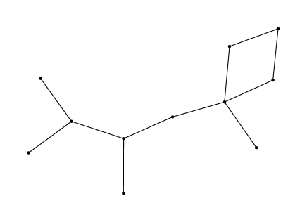
Figure 1: The ST-class of size 11 for maxdet matrices of order 26

Theorem 1.

For order $26$ there are at least $9923$ Hadamard classes of $\{+1,-1\}$ matrices with determinant $150\times 6^{11}\times 2^{25}$. They lie in at least $25$ switching classes, as given in Table $1$.

Proof.

The proof is computational. On our website [2] we give representatives of each of the $18$ ST-classes. From these “generators”, a program that implements switching can find all $5049$ HT-classes; this requires only 12 iterations of row/column switching and taking duals. By taking duals of the $7$ generators that are not self-dual, we obtain $25$ generators for the $9923$ H-classes. ∎

Order	#	Order	#	Order	#	Order	#
1	2823	2	4086	3	41	4	1840
6	151	8	607	12	106	16	143
24	20	32	44	36	6	39	1
48	13	64	13	72	8	78	6
96	3	108	1	156	2	216	2
288	4	576	2	22464	1

Table 2: Group orders of $9923$ H-classes for order 26

5 Results for order $27$

It is known that the maximal determinant $D(27)$ for order $27$ satisfies

$$546\leq\frac{D(27)}{6^{11}\times 2^{26}}<565,$$

where the lower bound is due to Tamura [23], and the upper bound is the (rounded up) Ehlich bound [8]. It is plausible to conjecture that the lower bound $546\times 6^{11}\times 2^{26}$ is maximal, since it is $0.9673$ of the Ehlich bound and has not been improved despite attempts using optimisation techniques that have been successful for other orders [18]. Unfortunately, proving that the lower bound is maximal seems difficult – the technique used in [3] to prove analogous results for orders $19$ and $37$ is impractical for order $27$ due to the size of the search space.

Tamura found a $\{+1,-1\}$ matrix $R$, with determinant $546\times 6^{11}\times 2^{26}$. The corresponding Gram matrix $G=RR^{T}$ has a block form with diagonal blocks of sizes $(7,7,7,6)$. Orrick [17] showed that Tamura’s matrix $R$ generates an ST-class ${\cal T}$ with $||{\cal T}||_{ST}=33$. The ST-class ${\cal T}$ splits into two S-classes, each containing 33 H-classes.

Using randomised decomposition of Tamura’s (conjectured maximal) Gram matrix, followed by switching, we have the following result.

Theorem 2.

There are at least $6489$ HT-classes $(12911$ H-classes$)$ of $\{\pm 1\}$ matrices of order 27 with determinant $546\times 6^{11}\times 2^{26}$. They lie in at least $204$ ST-classes $(388$ S-classes$)$. The largest ST-class contains at least $5765$ HT-classes $(11483$ H-classes$)$.

Proof.

The proof is computational. On our website [2] we give representatives of each of the $204$ ST-classes. From these “generators”, a program that implements switching can find all $6489$ HT-classes; this requires only 28 iterations of row/column switching and taking duals. By taking duals of the $184$ generators that are not self-dual, we obtain $388$ generators for the $12911$ H-classes. ∎

Details of the $204$ known ST-classes are summarised in Table 3. Twenty of these ST-classes are self-dual; the remaining $184$ each split into two S-classes. In the table, the columns headed “$||{\cal C}||_{ST}$” give the size of an ST-class $\cal C$, the next columns “#” give the number of such classes, and the columns “#split” give the number of these that split into two S-classes.

$||{\cal C}||_{ST}$	#	#split	$||{\cal C}||_{ST}$	#	#split	$||{\cal C}||_{ST}$	#	#split
5765	1	0	36	1	1	33	1	1
28	1	1	21	1	1	18	2	2
14	2	2	12	4	4	11	1	1
9	2	2	8	3	3	7	7	5
6	12	12	5	11	9	4	12	11
3	18	17	2	38	33	1	87	79

Table 3: 204 ST-classes for order 27

There is one “giant” class ${\cal G}$ of size 5765 HT-classes (11483 H-classes) and 203 small classes (maximum size 36 HT-classes). Tamura’s matrix $R$ generates the third-largest class, of size 33 HT-classes (66 H-classes). Unlike order 26 (see §4), there is no obvious subdivision of the classes into types.

Automorphism group orders for the 12911 H-classes are summarised in Table 4. Tamura’s matrix $R$ has group order $3$.

Order	multiplicity
1	12738
2	26
3	131
6	16

Table 4: Distribution of group orders for $12911$ H-classes

Figure 2: ST-classes of size 28 and 36 for matrices of order 27

6 Results for order $33$

For order $33$, the Barba bound (1) gives $D(33)<516\times 2^{74}$. Using the algorithm described in [3], we have shown that none of the $13670$ candidate Gram matrices $G$ satisfying $\det(G)^{1/2}\geq 470\times 2^{74}$ can decompose into a product $RR^{T}$, where $R\in\{+1,-1\}^{33\times 33}$. Thus, we have $D(33)<470\times 2^{74}$.

On the other hand, Solomon [21, 18] found a matrix $R\in\{+1,-1\}^{33\times 33}$ with $\det(R)=441\times 2^{74}$, which is greater than $0.9382$ of the upper bound. Thus, we know that

$$441\leq D(33)/2^{74}<470.$$

It is plausible to conjecture that the lower bound is best possible and $D(33)=441\times 2^{74}$. Proving this seems difficult, for reasons given in [3, §7.1]. In this section we find a large number of H-classes of solutions with determinant $441\times 2^{74}$. Even if the conjecture proves to be incorrect, the same techniques should be applicable to find many or all H-classes of solutions with larger determinant.

Starting from the Gram matrix $G=R^{T}R=RR^{T}$ corresponding to Solomon’s $\{+1,-1\}$ matrix $R$, our randomised tree search algorithm can find many solutions with the same determinant.

Using row/column switching and duality, we can find a huge number of inequivalent solutions. For example, starting from Solonon’s matrix $R$ and iterating the operation of row switching only, we found $37030740$ H-classes in 11 iterations before stopping our program because it was using too much memory. Clearly a different strategy is needed.

Exploring the switching graph using random walks

Given solutions $A_{0}$ and $B_{0}$, we can generate random walks $(A_{0},A_{1},A_{2},\ldots)$ and $(B_{0},B_{1},B_{2},\ldots)$ in the graph defined by row/column switching and transposition. Each vertex on a walk is connected by a row/column switching operation and possibly transposition to its successor.

If $A_{0}$ and $B_{0}$ are in different connected components, then the two random walks can not intersect. However, if $A_{0}$ and $B_{0}$ are in the same connected component, of size $s$ say, then we expect the two walks to intersect eventually, and probably after $O(\sqrt{s})$ steps unless the mixing time of the walks is too long (this depends on the geometry of the component, which is unknown).

Our implementation uses self-avoiding random walks. Each walk is stored in a hash table so we can quickly check if a new vertex has already been encountered in the same walk (in which case we try one of its neighbours) or in the other walk (in which case we have found an intersection). If, during a walk, all neighbours of the current vertex have been visited, then it is necessary to backtrack. This occurs rarely since the mean degree of a vertex is large (see below).

We fix $A_{0}=R$ and choose $B_{0}$ randomly. Usually (about 90% of the time) $R$ and $B_{0}$ are in the same connected component, nearly always the “giant” component ${\cal G}$. Otherwise, $B_{0}$ is in a “small” component (of size say $s$) and we discover this by being unable to continue the self-avoiding walk from $B_{0}$ past $B_{s-1}$.

In this way we find many vertices of the giant component ${\cal G}$, and also many “small” ST-classes.

We can gather statistics from the random walks. For example, we would like to estimate $||{\cal G}||_{ST}$, the total number of HT-classes (i.e. connected components) in the graph, the number of ST-classes, the mean degree of each vertex, etc.

If implemented as described above, the random walks are not uniform over the vertices of the connected components containing their starting points. They are approximately uniform over edges, so the probability of hitting a vertex $v$ depends on the degree $\deg(v)$.

We can either take this into account when gathering statistics, or avoid the problem by accepting a candidate vertex $v$ with probability $1/\deg(v)$. In this way the vertices are sampled uniformly if the walks are long enough. The drawback is that we have to compute the degrees of all candidate vertices (all neighbours of the current vertex), which might be time-consuming.

Results from random walks

We estimate that the overall size of the graph is $(3.08\pm 0.09)\times 10^{9}$ when measured in HT-classes. (In terms of H-classes the numbers are roughly doubled, since self-dual classes are rare.) The giant component ${\cal G}$ has size $||{\cal G}||_{ST}\approx(2.83\pm 0.08)\times 10^{9}$. In ${\cal G}$ the mean degree of each vertex is about $20$, so there are about $2.83\times 10^{10}$ edges.

We estimate that there are about $5\times 10^{7}$ small ST-classes, with mean size about 5. Of these we found more than $8\times 10^{4}$ so far, with the largest having size $2136$ (see Table 5).

We have found $1639$ singletons (ST-classes of size 1) and $5412$ self-dual matrices. One self-dual singleton was found.

The automorphism group orders observed during random walks are in $\{1,2,4\}$, with orders greater than $1$ being rare. Solomon’s $R$ has group order $2$.

Although most of these observations are imprecise, since they depend on random sampling, we can at least claim the following:

Theorem 3.

For order $33$ and determinant $441\times 2^{74}$, the ST-class ${\cal G}$ generated by Solomon’s matrix $R$ is self-dual and has size $||{\cal G}||_{ST}>197\times 10^{6}$. There are at least $8\times 10^{4}$ smaller ST-classes, $20$ of which are listed in Table $5$.

Proof.

As usual, the proof is computational. Starting from $R$, we found $197122852$ HT-classes in $9$ iterations of row/column switching and taking duals.

Starting random walks from $R$ and $R^{T}$, and performing row/column switching only, we found an intersection. Thus $R\leftrightarrow R^{T}$. It follows that $\cal G$ is self-dual. ∎

Remarks

1. Although $R$ is not self-dual, we found many self-dual matrices in the giant class $\cal G$ in the course of various random walks. Eight such matrices are at distance $3$ from $R$. The existence of a self-dual matrix in $\cal G$ is sufficient to show that $\cal G$ is self-dual.

size $s_{i}$	$\lambda_{i}$	size $s_{i}$	$\lambda_{i}$
2136	2	1100	1
1300	4	1069	2
1276	2	1011	1
1246	1	1008	1
1205	4	999	1(a)
1188	4	999	2(b)
1187	1	993	2
1148	2	958	2
1134	2	918	3
1104	2	909	3

Table 5: Some large ST-classes for order $33$

2. In addition to the giant class ${\cal G}$ of size about $2.83\times 10^{9}$, we found $20$ ST-classes of size $\geq 900$, as listed in Table 5, with the largest having size $2136$. Classes of the same size marked “(a)” and “(b)” are different, so there are (at least) two disjoint classes of size $999$.

3. Table 5 gives the number of times $\lambda_{i}$ that we found the same class of size $s_{i}$. This statistic is mentioned because it indicates how well we have sampled the search space. Excluding the giant class $\cal G$, the $20$ largest known classes, of total size $\sum s_{i}=22888$, were found $\sum\lambda_{i}=42$ times. Consider the union $U$ of these classes as a sample from the space, and assume that the space is sampled uniformly. Excluding the $20$ “hits” used to select $U$, there are $\sum(\lambda_{i}-1)=22$ additional “hits” on $U$. Thus, the fraction $\rho$ of the space sampled is $\rho\approx\sum(\lambda_{i}-1)/\sum s_{i}=22/22888\approx 1/1040$. Under our assumption, the probability $P$ of missing a given class of size $\geq 2136$ is bounded by

$$P\leq\left(1-\rho\right)^{2136}<\;{1}/{7}\,.$$ (5)

On the other hand, random sampling hit the giant class $1.04\times 10^{6}$ times, and the estimated size of this class is $2.83\times 10^{9}$, implying that $\rho\approx 1/2720$, so the estimate (5) on $P$ should be viewed with caution. The discrepancy between the two estimates of $\rho$ may be caused by nonuniformity of sampling and/or by an inaccurate estimate of the size of the giant class.

4. It would be interesting to know more about the graphs associated with “small” ST classes. We have observed one graph of size 3 (“$\vee$”), two of size 4 (“$\sqcup$” and “$\square$”), and only one of size 5 (“kite”). Figure 3 shows an example of each size in the range $10,\ldots,19$.

5. The reader may have noticed that the graphs displayed in Figures 1–3 are bipartite ($2$-colourable), although neato did not draw them in a way that makes this obvious. Computational experiments have shown that most, but not all, of the ST classes considered above have bipartite graphs. In particular, the graph of the giant component for order $33$ is not bipartite.

Acknowledgements

The author thanks Judy-anne Osborn for introducing him to the topic and for many stimulating discussions; Will Orrick and Paul Zimmermann for their ongoing collaboration; Brendan McKay for his graph isomorphism program nauty [15], which was used to check Hadamard equivalence; AT&T for the Graphviz graph visualization software, in particular neato, which was used to draw the figures; and the Mathematical Sciences Institute (ANU) for computer time on the cluster “orac”.

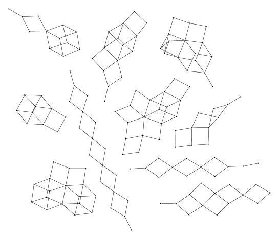
Figure 3: One ST-class of each size $10,\ldots,19$ for order $33$

References

- [1] G. Barba, Intorno al teorema di Hadamard sui determinanti a valore massimo, Giorn. Mat. Battaglini 71 (1933), 70–86.
- [2] R. P. Brent, The Hadamard maximal determinant problem, http://maths.anu.edu.au/~brent/maxdet/
- [3] R. P. Brent, W. P. Orrick, J. H. Osborn and P. Zimmermann, Maximal determinants and saturated D-optimal designs of orders and , submitted. Available from http://arxiv.org/abs/1112.4160.
- [4] R. P. Brent and J. H. Osborn, General lower bounds on maximal determinants of binary matrices, submitted. Available from http://arxiv.org/abs/1208.1805.
- [5] A. E. Brouwer, An infinite series of symmetric designs, Math. Centrum, Amsterdam, Report ZW 202/83 (1983).
- [6] R. H. F. Denniston, Enumeration of symmetric designs . In Algebraic and geometric combinatorics, Volume 65 of North-Holland Math. Stud., North-Holland, Amsterdam, 1982, 111–127.
- [7] H. Ehlich, Determinantenabschätzungen für binäre Matrizen, Math. Z. 83 (1964), 123–132.
- [8] H. Ehlich, Determinantenabschätzungen für binäre Matrizen mit , Math. Z. 84 (1964), 438–447.
- [9] J. Hadamard, Résolution d’une question relative aux déterminants, Bull. des Sci. Math. 17 (1893), 240–246.
- [10] N. Ito, J. S. Leon and J. Q. Longyear, Classification of 3-(24,12,5) designs and 24-dimensional Hadamard matrices, J. Combin. Theory Ser. A 31 (1981), 66–93.
- [11] H. Kimura, New Hadamard matrix of order 24, Graphs Combin. 5 (1989), 235–242.
- [12] C. Koukouvinos, S. Kounias and J. Seberry, Supplementary difference sets and optimal designs, Discrete Math. 88 (1991), 49–58.
- [13] S. Kounias, C. Koukouvinos, N. Nikolaou and A. Kakos, The non-equivalent circulant D-optimal designs for mod , , , J. Combin. Theory Ser. A 65 (1994), 26–38.
- [14] B. D. McKay, Hadamard equivalence via graph isomorphism, Discrete Mathematics 27 (1979), 213–214.
- [15] B. D. McKay, nauty User’s Guide (Version 2.4), Dept. of Computer Science, Australian National University, November 2009.
- [16] William P. Orrick, Switching operations for Hadamard matrices, SIAM J. Discrete Math. 22 (2008), 31–50.
- [17] William P. Orrick, On the enumeration of some D-optimal designs, J. Statist. Plann. Inference 138 (2008) 286–293. http://arxiv.org/abs/math/0511141v2
- [18] William P. Orrick, The Hadamard maximal determinant problem, http://www.indiana.edu/~maxdet/
- [19] Judy-anne H. Osborn, The Hadamard Maximal Determinant Problem, Honours Thesis, University of Melbourne, 2002, 142 pp. http://wwwmaths.anu.edu.au/~osborn/publications/pubsall.html
- [20] R. E. A. C. Paley, On orthogonal matrices, J. Math. Phys 12 (1933), 311–320.
- [21] B. Solomon, Personal communication to W. Orrick, 18 June 2002.
- [22] E. Spence, Skew-Hadamard matrices of the Goethals-Siedel type, Canadian J. Math. 27 (1975), 555–560.
- [23] H. Tamura, Personal communication to W. Orrick, 26 August 2005.
- [24] Ian M. Wanless, Cycle switches in latin squares, Graphs Combin. 20 (2004), 545–570.
- [25] A. L. Whiteman, A family of D-optimal designs, Ars Combinatoria 30 (1990), 23–26.
- [26] W. Wojtas, On Hadamard’s inequality for the determinants of order non-divisible by , Colloq. Math. 12 (1964), 73–83.
- [27] C. H. Yang, On designs of maximal -matrices of order (mod ), Math. Comp. 22 (1968), 174–180.