Fermionic impurities in Chern-Simons-matter theories

Paolo Benincasa and Alfonso V. Ramallo

Departamento de Física de Partículas, Universidade de Santiago de Compostela
and
Instituto Galego de Física de Altas Enerxías (IGFAE)
E-15782, Santiago de Compostela, Spain

Abstract

We study the addition of quantum fermionic impurities to the ${\cal N}=6$ supersymmetric Chern-Simons-matter theories in $2+1$ spacetime dimensions. The impurities are introduced by means of Wilson loops in the antisymmetric representation of the gauge group. In a holographic setup, the system is represented by considering D6-branes probing the $AdS_{4}\times{\mathbb{C}}{\mathbb{P}}^{3}$ background of type IIA supergravity. We study the thermodynamic properties of the system and show how a Kondo lattice model with holographic dimers can be constructed. By computing the Kaluza-Klein fluctuation modes of the probe brane we determine the complete spectrum of dimensions of the impurity operators. A very rich structure is found, depending both on the Kaluza-Klein quantum numbers and on the filling fraction of the impurities.

1 Introduction

The gauge/gravity correspondence [1, 2] has been an invaluable analytic tool which has provided new insights on the the dynamics of gauge theories in the strong coupling regime. Indeed, in the framework of string theory, the gauge symmetry is realized as the worldvolume symmetry of a stack of coincident branes and the corresponding gravitational background encodes relevant properties of the gauge theory in the ’t Hooft limit. The richness of string theory allows several possibilities to deform the theory by adding extra degrees of freedom. In particular, one can add new sets of branes which intersect with the color branes that host the gauge symmetry and create a defect in the gauge theory. By studying the dynamics of the extra branes in the original background one can extract useful dynamical information of the corresponding gauge theory with impurities.

In this paper we will concentrate on analyzing the case in which the defects are point-like. The canonical example of this type of systems is ${\cal N}=4$ Super-Yang-Mills (SYM) with fermionic impurities. The brane realization of this system is obtained by adding D5-branes to the $AdS_{5}\times S^{5}$ background, dual to ${\cal N}=4$ SYM. The D5-branes are extended in the holographic direction and wrap an ${\mathbb{S}}^{4}$ inside the ${\mathbb{S}}^{5}$ in such a way that their worldvolume is an $AdS_{2}\times{\mathbb{S}}^{4}$ submanifold of $AdS_{5}\times{\mathbb{S}}^{5}$ [3, 4]. The ${\mathbb{S}}^{4}$ that the D5-branes wrap are obtained by fixing the latitude inside the ${\mathbb{S}}^{5}$ to a discrete set of angles, which are obtained by imposing a quantization condition [4]. These configurations can be regarded as describing bound states of fundamental strings extended along the holographic coordinate. Equivalently, they represent Wilson lines in the antisymmetric representation of the $SU(N)$ gauge group of the ${\cal N}=4$ SYM theory [5]. As shown in detail in [6], these Wilson loops can be obtained by integrating out a fermionic impurity, which is localized in the spatial gauge theory directions and whose occupation number is just the number of strings carried by the D5-brane. More recently, these configurations have been utilized [7, 8] to construct holographic dimer models, by considering D5-branes which connect two spatially separated impurities on the boundary of $AdS_{5}$. It has been also argued that this setup of D3- and D5-branes realizes holographically the maximally supersymmetric Kondo model [9, 10] (see also [11, 12]).

The holographic study of gauge theories with impurities may be useful to understand the applications of the AdS/CFT correspondence to condensed matter theories. For this reason it is very important to have examples of such systems at our disposal, in which both sides of the correspondence are clearly identified and one can perform non-trivial tests of the duality. Following this line of thought, we study in this paper the addition of fermionic impurities to the ${\cal N}=6$ Chern-Simons-matter theory proposed by Aharony et al. (ABJM) in ref. [13] (based on previous results by Bagger and Lambert [14] and Gustavsson [15]). The ABJM theory describes the dynamics of multiple M2-branes at a ${\mathbb{C}}^{4}/{\mathbb{Z}}_{k}$ singularity and is a $U(N)\times U(N)$ (2+1)-dimensional Chern-Simons gauge theory with levels $(k,-k)$ and bifundamental matter fields. In the large $N$ limit this theory admits a supergravity description in M-theory in terms of the $AdS_{4}\times{\mathbb{S}}^{7}/{\mathbb{Z}}_{k}$ geometry with flux. Moreover, when the Chern-Simons level $k$ is large the system is better described in terms of type IIA supergravity. In this ten-dimensional description the geometry is of the form $AdS_{4}\times{\mathbb{C}}{\mathbb{P}}^{3}$ with fluxes of the RR two- and four- forms.

It was proposed in ref. [16] that the Wilson lines in the antisymmetric representations of the gauge group of the ABJM theory are holographically realized as D6-branes extended along an $AdS_{2}\subset AdS_{4}$ and wrapping a five-dimensional submanifold of ${\mathbb{C}}{\mathbb{P}}^{3}$. These are, therefore, the natural brane configurations to consider in order to construct the holographic dual of the Chern-Simons-matter theory with fermionic impurities. In this paper we will confirm this identification and we will study in detail some of the properties of the system with impurities. This brane setup constitutes the holographic description of a Kondo model in which the impurities are coupled to an ambient interacting CFT in three spacetime dimensions.

In the configurations we will focus on, the probe D6-branes capture part of the RR flux of the background and, as a consequence, an electric worldvolume field must be turned on. This worldvolume field can be eliminated from the lagrangian of the probe by means of a Legendre transformation, after using the quantization condition found in [4]. The result is an effective one-dimensional problem which can be solved by means of a first-order BPS differential equation which depends on the quantization integer $n$ (that represents the number of fundamental strings). In this paper we will mostly center in studying the simplest solutions of the BPS equation, which give rise to flux tubes made of $n$ strings with $0<n<N$ ($N$ is the rank of the $U(N)$ gauge groups). There are, however, more general solutions which are related to the baryon vertex of the ABJM theory. A first analysis of these baryonic solutions is relegated to an appendix. We will leave a more complete study for future work.

In the flux tube solutions used to create the impurities, the embedding of the D6-branes is such that one of the angular coordinates that parametrize the ${\mathbb{C}}{\mathbb{P}}^{3}$ is fixed to a constant which depends on the number $n$ of strings. In the dual field theory $n$ is just the number of defect fermions and the ratio $n/N$ is the filling fraction of the impurities. The D6-branes wrap a squashed $T^{1,1}$ space inside the internal ${\mathbb{C}}{\mathbb{P}}^{3}$. Recall that the $T^{1,1}$ space is a five-dimensional Sasaki-Einstein space whose metric can be represented as a $U(1)$ fibration of ${\mathbb{S}}^{2}\times{\mathbb{S}}^{2}$. In our case this space is internally deformed by squashing factors which preserve the fiber structure and depend non-trivially on the filling fraction of the impurities.

Once the setup required to add impurities is clearly identified, one can study many properties of the system. We will first analyze its thermodynamic properties by considering a probe brane in a black hole background dual to the ABJM theory at finite temperature. We will also study the configurations in which two flux tubes ending on two different points on the boundary of $AdS_{4}$ are connected in the bulk and we will show that there exists a dimerization transition similar to the one described in refs. [7, 8]. In order to establish the stability of the brane configuration, we will analyze in detail the fluctuations of a brane probe at zero temperature. We will be able to decouple the different modes and read the conformal dimensions of the various dual operators. To carry out this analysis we will have to develop the harmonic calculus on the squashed $T^{1,1}$ space. As a result we will uncover a rich structure which depends both on the filling fraction of the impurities and on the quantum numbers of the Kaluza-Klein harmonics of the squashed $T^{1,1}$. As happens in other conifold-like theories, the conformal dimensions will not be, in general, rational numbers [17]. We will be able to characterize the normalizable modes which do correspond to impurity operators of rational dimensions. These operators should be the ones protected by the supersymmetry of the system.

The rest of this paper is organized as follows. In section 2 we briefly review the gravity dual of the ABJM theory in the type IIA supergravity. In section 3 we study a class of configurations of the probe D6-branes in which they wrap a co-dimension one submanifold of ${\mathbb{C}}{\mathbb{P}}^{3}$. Section 4 is devoted to analyzing the flux tube embeddings. The thermodynamic properties of these configurations are studied in section 5 by considering embeddings in the black hole version of the ABJM metric. In this section we compute holographically the free energy and entropy of the impurity. In section 6 we study D6-brane embeddings in which the brane is hanging from the boundary and ends on two different points. In this section we compute the free energy of this hanging tube configuration and we explore the corresponding dimerization transition. In sections 7 and 8 we analyze in detail the fluctuation modes of the D6-branes around the flux tube and dimer configurations at zero temperature. We check their stability and compute the conformal dimensions of the dual impurity fields. In section 9 we summarize our results, extract some conclusions and point out some lines for possible future research. The paper is completed with several appendices. In appendix A we briefly present the BPS worldvolume equation and find its solutions. In appendix B we derive the lagrangian for the fluctuations of the probe brane. In appendix C we study the laplacian for the squashed $T^{1,1}$. In appendix D we develop the harmonic calculus for these spaces. Finally, in appendix E we review some basic facts about Heun’s equation and its connection to a quantum integrable model.

2 The ABJM background

The ABJM background [13] of type IIA string theory is characterized by a ten-dimensional metric of the form $AdS_{4}\times{\mathbb{C}}\,{\mathbb{P}}^{3}$:

$$ds^{2}\,=\,{R^{3}\over 4k}\,(ds^{2}_{AdS_{4}}\,+\,4\,ds^{2}_{{\mathbb{C}}{\mathbb{P}}^{3}})\,\,,$$ (2.1)

where $ds^{2}_{AdS_{4}}$ and $ds^{2}_{{\mathbb{C}}{\mathbb{P}}^{3}}$ are, respectively, the $AdS_{4}$ and ${\mathbb{C}}{\mathbb{P}}^{3}$ metrics. The former can be written, in Poincaré coordinates, as:

$$ds^{2}_{AdS_{4}}\,=\,r^{2}\,\big{(}\,-dt^{2}+dx^{2}+dy^{2}\,\big{)}\,+\,{dr^{2}\over r^{2}}\,\,.$$ (2.2)

In (2.1) we have represented the $AdS_{4}$ radius in terms of $R$ and $k$. Actually, the ABJM solution depends on two integers $N$ and $k$ which correspond, in the dual gauge theory, to the rank of the gauge groups and to the Chern-Simons levels, respectively. The $AdS_{4}$ radius in (2.1) can be written in terms of these two integers as:

$${R^{3}\over 4k}\,=\,\pi\,\sqrt{{2N\over k}}\,\,,$$ (2.3)

where we are taking the Regge slope $\alpha^{\prime}=1$. The metric $ds^{2}_{{\mathbb{C}}{\mathbb{P}}^{3}}$ in (2.1) is the canonical Fubini-Study metric. In order to write its expression in a convenient form, let us consider four complex coordinates $z^{i}$ ($i=1,\cdots,4$) such that $\sum_{i}\,|z^{i}|^{2}\,=\,1$. Therefore, these $z^{i}$’s parametrize a seven-sphere. We will represent them as:

$$z^{1}\,=\,\cos{\alpha\over 2}\,\cos{\theta_{1}\over 2}\,e^{{i\over 4}\,(2\varphi_{1}\,+\,\chi\,+\,\xi)}\,\,,\qquad z^{2}\,=\,\cos{\alpha\over 2}\,\sin{\theta_{1}\over 2}\,e^{{i\over 4}\,(-2\varphi_{1}\,+\,\chi\,+\,\xi)}\,\,,$$

$$z^{3}\,=\,\sin{\alpha\over 2}\,\sin{\theta_{2}\over 2}\,e^{{i\over 4}\,(2\varphi_{2}\,-\,\chi\,+\,\xi)}\,\,,\qquad z^{4}\,=\,\sin{\alpha\over 2}\,\cos{\theta_{2}\over 2}\,e^{{i\over 4}\,(-2\varphi_{2}\,-\,\chi\,+\,\xi)}\,\,.$$ (2.4)

It is straightforward to verify that the metric of the seven sphere ${\mathbb{S}}^{7}$ can be written in these coordinates as a $U(1)$ bundle over ${{\mathbb{C}}{\mathbb{P}}^{3}}$, namely:

$$ds^{2}_{{\mathbb{S}}^{7}}\,=\,\,ds^{2}_{{\mathbb{C}}{\mathbb{P}}^{3}}\,+\,(d\zeta+A)^{2}\,\,.$$ (2.5)

In our parametrization $\zeta\sim\xi$ and the ${{\mathbb{C}}{\mathbb{P}}^{3}}$ metric $ds^{2}_{{\mathbb{C}}{\mathbb{P}}^{3}}$, as well as the $U(1)$ connection $A$, are given by:

$$ds^{2}_{{\mathbb{C}}{\mathbb{P}}^{3}}\,=\,{1\over 4}\,\Big{[}\,d\alpha^{2}\,+\,\cos^{2}{\alpha\over 2}\,\big{(}\,d\theta_{1}^{2}\,+\,\sin^{2}\theta_{1}\,d\varphi_{1}^{2}\,\big{)}\,+\,\sin^{2}{\alpha\over 2}\,\big{(}\,d\theta_{2}^{2}\,+\,\sin^{2}\theta_{2}\,d\varphi_{2}^{2}\,\big{)}\,+\,$$

$$\qquad\qquad\qquad\qquad+\sin^{2}{\alpha\over 2}\,\cos^{2}{\alpha\over 2}\,\big{(}\,d\chi+\cos\theta_{1}d\varphi_{1}\,+\,\cos\theta_{2}d\varphi_{2}\,\big{)}^{2}\,\,\Big{]}\,\,,$$

$$A\,=\,\cos\alpha\,d\chi\,+\,2\,\cos^{2}{\alpha\over 2}\,\cos\theta_{1}d\varphi_{1}\,-\,2\,\sin^{2}{\alpha\over 2}\,\cos\theta_{2}\,d\varphi_{2}\,\,.$$ (2.6)

The ranges of the angles are $0\leq\alpha,\theta_{1},\theta_{2},\leq\pi$, $0\leq\varphi_{1},\varphi_{2}<2\pi$ and $0\leq\chi<4\pi$. Notice that, in the representation (2.6), the submanifolds with $\alpha={\rm constant}$ are squashed $T^{1,1}$ five-dimensional spaces, which foliate the entire ${\mathbb{C}}{\mathbb{P}}^{3}$.

The ABJM type IIA background is also endowed with RR two- and four- forms $F_{2}$ and $F_{4}$, as well as a constant dilaton $\phi$, which are given by:

$$e^{2\phi}\,=\,{R^{3}\over k^{3}}\,\,,\qquad F_{4}\,=\,{3\over 8}\,R^{3}\,\,\Omega_{AdS_{4}}\,\,,\qquad F_{2}\,=\,{k\over 4}\,dA\,\,,$$ (2.7)

where $\Omega_{AdS_{4}}$ is the volume element of the $AdS_{4}$ metric (2.2). This background is a good supergravity dual of the Chern-Simons matter theory when the $AdS_{4}$ radius is large in string units (and the corresponding curvature is small) and when the string coupling $e^{\phi}$ is small. From (2.3) and (2.7) it follows [13] that these conditions are satisfied when $N^{{1\over 5}}<<k<<N$.

In type IIA supergravity the RR six-form $F_{6}$ is defined as the Hodge dual of the RR four-form $F_{4}$. For the ABJM background $F_{6}$ is given by:

$$F_{6}\,=\,{}^{*}\,F_{4}\,=\,{3R^{6}\over 2^{8}k}\,\sin^{3}\alpha\,d\alpha\wedge\epsilon_{5}\,\,,$$ (2.8)

where $\epsilon_{5}$ is the five-form:

$$\epsilon_{5}\,=\,\sin\theta_{1}\sin\theta_{2}\,d\theta_{1}\wedge d\theta_{2}\wedge d\chi\wedge d\varphi_{1}\wedge d\varphi_{2}\,\,.$$ (2.9)

Let us now find the five-form potential $C_{5}$ for $F_{6}$ (i.e. such that $F_{6}=dC_{5}$). This potential will be very useful in the analysis of the probe D6-branes of section 3. First of all, we define the function $C(\alpha)$ as the solution of the following first-order equation:

$${dC\over d\alpha}\,=\,-3\,\big{(}\sin\alpha\big{)}^{3}\,\,,\qquad\qquad C(0)=0\,\,.$$ (2.10)

This function is just:

$$C(\alpha)\,=\,\cos\alpha\big{(}\sin^{2}\alpha\,+\,2)\,-\,2\,\,.$$ (2.11)

Then, it is immediate to verify that the RR potential five-form $C_{5}$ can be taken as:

$$C_{5}\,=\,-{R^{6}\over 2^{8}\,k}\,C(\alpha)\,\epsilon_{5}\,\,.$$ (2.12)

3 D6-brane probes

Let us consider a D6-brane extended along the radial direction $r$ and wrapping a five-dimensional submanifold inside the ${\mathbb{C}}{\mathbb{P}}^{3}$ at fixed values of the Minkowski coordinates $x,y$. Notice that a configuration of this type creates a point-like defect in the gauge theory. In order to describe it in detail, we will take the following worldvolume coordinates:

$$\zeta^{a}\,=\,(t,r,\gamma^{i})\,=\,(t,r,\theta_{1},\varphi_{1},\theta_{2},\varphi_{2},\chi)\,\,.$$ (3.1)

We will consider embeddings in which the angle $\alpha$ is a function of the radial coordinate $r$, namely:

$$\alpha\,=\,\alpha(r)\,\,.$$ (3.2)

Notice that the hypersurface $\alpha={\rm constant}$ defines a co-dimension one submanifold of the internal ${\mathbb{C}}{\mathbb{P}}^{3}$. In addition, we will switch on an electric worldvolume gauge field $F_{0r}$. Actually, such a worldvolume field is sourced by the RR potential $C_{5}$ through the Wess-Zumino (WZ) term of the D6-brane action (see below). The Dirac-Born-Infeld (DBI) piece of the brane action is just:

$$S_{DBI}\,=\,-T_{D_{6}}\,\int d^{7}\zeta\,e^{-\phi}\,\sqrt{-\det(g+F)}\,\,,$$ (3.3)

where $g$ is the induced metric on the worldvolume of the D6-brane and $T_{6}$ is its tension. The DBI determinant, integrated over the five angles $\gamma^{i}$ in (3.1) is:

$$T_{D_{6}}\,\int d^{5}\,\gamma\,e^{-\phi}\,\sqrt{-\det(g+F)}\,=\,{R^{9}\over 2^{10}\,\pi^{3}\,k^{2}}\,\,\big{(}\sin\alpha\big{)}^{3}\,\,\sqrt{1+r^{2}\,\big{(}\alpha^{\prime}\big{)}^{2}\,-\,{16k^{2}\over R^{6}}\,F_{0r}^{2}}\,\,,$$ (3.4)

where $d^{5}\gamma=d\theta_{1}\wedge d\theta_{2}\wedge d\chi\wedge d\varphi_{1}\wedge d\varphi_{2}$ and $\alpha^{\prime}$ denotes $d\alpha/dr$. Let us define the effective DBI lagrangian density ${\cal L}_{DBI}$ as:

$$S_{DBI}\,=\,\int dtdr\,{\cal L}_{DBI}\,\,.$$ (3.5)

Then, one has:

$${\cal L}_{DBI}\,=\,-{R^{9}\over 2^{10}\,\pi^{3}\,k^{2}}\,\,\big{(}\sin\alpha\big{)}^{3}\,\,\sqrt{1+r^{2}\,\big{(}\alpha^{\prime}\big{)}^{2}\,-\,{16k^{2}\over R^{6}}\,F_{0r}^{2}}\,\,.$$ (3.6)

Moreover, the WZ action is:

$$S_{WZ}\,=\,T_{6}\,\int C_{5}\wedge F\,\equiv\int dr\,dt\,{\cal L}_{WZ}\,\,.$$ (3.7)

By using the expression of $C_{5}$ written in (2.12), one arrives at the following expression of ${\cal L}_{WZ}$:

$${\cal L}_{WZ}\,=\,-{R^{6}\over 2^{8}\,\pi^{3}\,k}\,C(\alpha)\,F_{0r}\,\,.$$ (3.8)

Then, the total lagrangian density ${\cal L}\,=\,{\cal L}_{DBI}+{\cal L}_{WZ}$ can be written as:

$${\cal L}\,=\,-{R^{6}\over 2^{8}\,\pi^{3}\,k}\,\Bigg{[}\,{R^{3}\over 4k}\,\big{(}\sin\alpha\big{)}^{3}\,\sqrt{1+r^{2}\,\big{(}\alpha^{\prime}\big{)}^{2}\,-\,{16k^{2}\over R^{6}}\,F_{0r}^{2}}\,+\,C(\alpha)\,F_{0r}\,\Bigg{]}\,\,.$$ (3.9)

The equation of motion of the gauge field derived from the lagrangian density (3.9) implies that:

$${\partial{\cal L}\over\partial F_{0r}}\,=\,{\rm constant}\,\,,$$ (3.10)

which is nothing but the Gauss law. By using the quantization condition derived in [4], one can relate this constant to the number $n$ of strings (quarks) of the flux tube, namely:

$${\partial{\cal L}\over\partial F_{0r}}\,=\,n\,T_{f}\,\,,$$ (3.11)

where $T_{f}$ is the tension of the fundamental string and $n\in{\mathbb{Z}}$ is the fundamental string charge carried by the D6-brane. For our lagrangian density (3.9) we get:

$${\partial{\cal L}\over\partial F_{0r}}\,=\,{R^{6}\over 2^{8}\,\pi^{3}\,k}\,\Bigg{[}\,{4k\over R^{3}}\,{F_{0r}\,\big{(}\sin\alpha\big{)}^{3}\over\sqrt{1+r^{2}\,\big{(}\alpha^{\prime}\big{)}^{2}\,-\,{16k^{2}\over R^{6}}\,F_{0r}^{2}}}\,-\,C(\alpha)\,\Bigg{]}\,\,.$$ (3.12)

By using this expression in (3.11) we can determine $F_{0r}$ in terms of the other variables. Indeed, let us define the function ${\cal C}_{n}(\alpha)$ as:

$${\cal C}_{n}(\alpha)\,\equiv C(\alpha)\,+\,{4n\over N}\,\,,$$ (3.13)

whose explicit expression is:

$${\cal C}_{n}(\alpha)\,=\,\cos\alpha\big{(}\sin^{2}\alpha\,+\,2)\,-\,2\,+\,{4n\over N}\,\,.$$ (3.14)

Notice that ${\cal C}_{n}(\alpha)$ satisfies the equation:

$${d{\cal C}_{n}(\alpha)\over d\alpha}\,=\,-3\,\big{(}\sin\alpha\big{)}^{3}\,\,,\qquad\qquad{\cal C}_{n}(0)\,=\,{4n\over N}\,\,.$$ (3.15)

By combining (3.11) and (3.12) one can get a expression of $F_{0r}$ in terms of the function ${\cal C}_{n}(\alpha)$, namely:

$$F_{0r}\,=\,{R^{3}\over 4k}\,{\sqrt{1\,+\,r^{2}\,\big{(}\alpha^{\prime}\big{)}^{2}}\over\sqrt{\big{(}\sin\alpha\big{)}^{6}\,+\,{\cal C}_{n}(\alpha)^{2}}}\,\,{\cal C}_{n}(\alpha)\,\,.$$ (3.16)

In order to eliminate the electric field from the equations of motion, let us next compute the hamiltonian of the system by performing the Legendre transformation of the lagrangian density (3.9):

$$H\,=\,\int dr\,\Big{[}\,F_{0r}\,{\partial{\cal L}\over\partial F_{0r}}\,-\,{\cal L}\,\Big{]}\,\equiv\,\int dr\,{\cal H}\,\,.$$ (3.17)

By explicit calculation, one gets:

$$F_{0r}\,{\partial{\cal L}\over\partial F_{0r}}\,-\,{\cal L}\,=\,{R^{9}\over 2^{10}\,\pi^{3}\,k^{2}}\,\,\,{1\,+\,r^{2}\,\big{(}\alpha^{\prime}\big{)}^{2}\over\sqrt{1\,+\,r^{2}\,\big{(}\alpha^{\prime}\big{)}^{2}\,-\,{16k^{2}\over R^{6}}\,F_{0r}^{2}}}\,\,\,\big{(}\sin\alpha\big{)}^{3}\,\,.$$ (3.18)

Moreover, from the expression of $F_{0r}$ written in (3.16), we deduce:

$${\big{(}\sin\alpha\big{)}^{3}\over\sqrt{1\,+\,r^{2}\,\big{(}\alpha^{\prime}\big{)}^{2}\,-\,{16k^{2}\over R^{6}}\,F_{0r}^{2}}}\,=\,{\sqrt{\big{(}\sin\alpha\big{)}^{6}\,+\,{\cal C}_{n}(\alpha)^{2}}\over\sqrt{1\,+\,r^{2}\,\big{(}\alpha^{\prime}\big{)}^{2}}}\,\,.$$ (3.19)

Thus, the hamiltonian density ${\cal H}$ can be written as:

$${\cal H}\,=\,{R^{9}\over 2^{10}\,\pi^{3}\,k^{2}}\,\,\,\sqrt{1\,+\,r^{2}\,\big{(}\alpha^{\prime}\big{)}^{2}}\,\,\sqrt{\big{(}\sin\alpha\big{)}^{6}\,+\,{\cal C}_{n}(\alpha)^{2}}\,\,.$$ (3.20)

The different embeddings of the D6-brane described by our ansatz can be found by integrating the Euler-Lagrange equation derived from (3.20). In the main part of this paper we will concentrate on studying the simplest of these configurations, namely those for which $\alpha$ is a constant. These embeddings will be analyzed in detail in following sections. In appendix A we will present embeddings with non-constant $\alpha$, which satisfy a first-order BPS equation. These last configurations are related to the baryon vertex of the ABJM theory (see [18, 19] for a similar analysis in the $AdS_{5}\times S^{5}$ background). We will leave their detailed study for a future work.

4 Flux tube configurations

Let us now look for solutions of the equations of motion which have a constant $\alpha$ angle. Clearly, we should require that:

$${\partial{\cal H}\over\partial\alpha}\Big{|}_{\alpha^{\prime}=0}\,=\,0\,\,.$$ (4.1)

Therefore, we need to compute the derivative of the second square root in (3.20). With this purpose in mind, we define the following function:

$$\Lambda_{n}(\alpha)\,\equiv\,\big{(}\sin\alpha\big{)}^{2}\,\cos\alpha\,-\,{\cal C}_{n}(\alpha)\,\,.$$ (4.2)

As:

$${d\over d\alpha}\,\,\Big{[}\,\big{(}\sin\alpha\big{)}^{6}\,+\,{\cal C}_{n}(\alpha)^{2}\,\Big{]}\,=\,6\,\big{(}\sin\alpha\big{)}^{3}\,\Lambda_{n}(\alpha)\,\,,$$ (4.3)

we get:

$${\partial{\cal H}\over\partial\alpha}\Big{|}_{\alpha^{\prime}=0}\,=\,{3\,R^{9}\over 2^{10}\,\pi^{3}\,k^{2}}\,\,{\big{(}\sin\alpha\big{)}^{3}\over\sqrt{\big{(}\sin\alpha\big{)}^{6}\,+\,{\cal C}_{n}(\alpha)^{2}}}\,\,\Lambda_{n}(\alpha)\,\,.$$ (4.4)

Therefore, the non-trivial configurations with constant $\alpha$ occur when $\alpha=\alpha_{n}$, where $\alpha_{n}$ is a solution of the equation:

$$\Lambda_{n}(\alpha_{n})\,=\,0\,\,.$$ (4.5)

Let us now study the solutions of this equation. By plugging the definition of ${\cal C}_{n}(\alpha)$ written in (3.14) into (4.2), one can obtain the explicit expression of $\Lambda_{n}(\alpha)$, which is given by:

$$\Lambda_{n}(\alpha)\,=\,2\,\,\Big{(}\,1\,-\,{2n\over N}\,-\,\cos\alpha\,\Big{)}\,\,.$$ (4.6)

Thus, the roots of (4.5) are:

$$\cos\alpha_{n}\,=\,1\,-\,{2n\over N}\,\,.$$ (4.7)

Notice that there is a unique solution $\alpha_{n}\in[0,\pi]$ for every $n$ in the range $0\leq n\leq N$. This configuration was proposed in reference [16] as the holographic dual of the Wilson loop of the ABJM theory in the antisymmetric representations of the gauge group. The fact that $n\leq N$ supports this identification and is a manifestation of the so-called stringy exclusion principle. The energy density for these configurations is just:

$$E_{n}\,\equiv\,{\cal H}(\alpha=\alpha_{n})\,=\,{N\over 8\pi}\,{R^{3}\over 4k}\,\,\big{(}\sin\alpha_{n}\big{)}^{2}\,\,.$$ (4.8)

Using the value of $\alpha_{n}$ written in (4.7), we get the following binomial law for the energy density:

$$E_{n}\,=\,\sqrt{\lambda\over 2}\,\,{n(N-n)\over N}\,\,,$$ (4.9)

where we have written the result in terms of the ’t Hooft coupling $\lambda$ of the Chern-Simons-matter theory ($\lambda=N/k$). Notice that $E_{n}$ is invariant under the change $n\rightarrow N-n$, as it should for the holographic dual of an object transforming in the anti-symmetric representation of the gauge group. Notice also that for small $n$ (or large $N$) the energy density $E_{n}$ is just equal to $n$ times the tension of a fundamental string extended along the radial direction in the geometry (2.1) (which is given by $T_{f}\,R^{3}/4k\,=\,\sqrt{\lambda/2}$). This is, again, in favor of the interpretation of this configuration as a bound state of fundamental strings, as those studied in [4] for backgrounds generated by Dp-branes. The fact that $E_{n}\leq nT_{f}\,R^{3}/4k$ is indicating that the formation of the bound state is energetically favored and that the configuration is stable. We will check explicitly this stability by computing the fluctuation spectra of the brane in section 7. It is also interesting to point out here that, as checked explicitly in [16], these configurations are 1/6 BPS, i.e. they preserve four real supercharges.

The constant electric field $\bar{f}_{0r}$ corresponding to this configuration can be obtained from (3.16) by substituting $\alpha$ by $\alpha_{n}$, namely:

$$\bar{f}_{0r}\,=\,{R^{3}\over 4k}\,\,\cos\alpha_{n}\,\,.$$ (4.10)

Notice that the induced metric on the D6-brane worldvolume takes the form:

$$ds^{2}\,=\,{R^{3}\over 4k}\,\,\Big{[}\,-\,r^{2}\,dt^{2}\,+\,{dr^{2}\over r^{2}}\,+\,ds^{2}_{\tilde{T}^{1,1}}\,\Big{]}\,\,,$$ (4.11)

which is of the form $AdS_{2}\times\tilde{T}^{1,1}$, with $\tilde{T}^{1,1}$ being a squashed $T^{1,1}$ space, with metric:

$$ds^{2}_{\tilde{T}^{1,1}}\,=\,\tilde{g}_{ij}\,d\gamma^{i}\,d\gamma^{j}\,=\,\cos^{2}{\alpha_{n}\over 2}\,\big{(}\,d\theta_{1}^{2}\,+\,\sin^{2}\theta_{1}\,d\varphi_{1}^{2}\,\big{)}\,+\,\sin^{2}{\alpha_{n}\over 2}\,\big{(}\,d\theta_{2}^{2}\,+\,\sin^{2}\theta_{2}\,d\varphi_{2}^{2}\,\big{)}\,+\,$$

$$\qquad\qquad\qquad\qquad\qquad\qquad+\sin^{2}{\alpha_{n}\over 2}\,\cos^{2}{\alpha_{n}\over 2}\,\big{(}\,d\chi+\cos\theta_{1}d\varphi_{1}\,+\,\cos\theta_{2}d\varphi_{2}\,\big{)}^{2}\,\,\,.$$ (4.12)

Taking into account that the angles $\alpha_{n}$ in (4.7) satisfy:

$$\sin^{2}{\alpha_{n}\over 2}\,=\,{n\over N}\,\,,\qquad\qquad\cos^{2}{\alpha_{n}\over 2}\,=\,{N-n\over N}\,\,,$$ (4.13)

it follows that the metric $ds^{2}_{\tilde{T}^{1,1}}$ can be written in the form:

$$ds^{2}_{\tilde{T}^{1,1}}\,=\,{N-n\over N}\,\,\big{(}\,d\theta_{1}^{2}\,+\,\sin^{2}\theta_{1}\,d\varphi_{1}^{2}\,\big{)}\,+\,{n\over N}\,\,\big{(}\,d\theta_{2}^{2}\,+\,\sin^{2}\theta_{2}\,d\varphi_{2}^{2}\,\big{)}\,+\,$$

$$\qquad\qquad\qquad\qquad\qquad\qquad+\,{n(N-n)\over N^{2}}\,\big{(}\,d\chi+\cos\theta_{1}d\varphi_{1}\,+\,\cos\theta_{2}\,d\varphi_{2}\,\big{)}^{2}\,\,\,.$$ (4.14)

Notice that the line element in (4.14) collapses to the one of to a two-sphere when $n=0,N$. This implies that the corresponding D6-brane configurations are singular and, accordingly, we will assume from now on that $0<n<N$. Moreover, the metric (4.14) displays the following symmetry:

$$(\theta_{1},\varphi_{1})\,\,\leftrightarrow\,\,(\theta_{2},\varphi_{2})\,\,,\qquad\qquad\qquad n\,\,\leftrightarrow\,\,N-n\,\,.$$ (4.15)

The configuration of D6-branes described above creates a point-like defect in the bulk Chern-Simons matter theory. The $n$ fundamental strings carried out by the D6-branes introduce $n$ fermions localized on the defect, which can be regarded as fermionic impurities in the Chern-Simons-matter theory. As pointed out in [6] for the similar configurations in ${\cal N}=4$ SYM, by integrating out the defect fermions one should get an effective theory for the bulk fields in which there is an insertion of a Wilson loop in the antisymmetric representation of the gauge group. This argument establishes a correspondence between the Wilson loop interpretation of these configurations (as proposed in [16]) and the model of quantum impurities developed in this paper. Notice that our setup describes a Kondo model in which the ambient theory is an interacting supersymmetric Chern-Simons-matter theory. The ratio:

$$\nu\,=\,{n\over N}\,\,,$$ (4.16)

will be referred to as the filling fraction. Notice that the metric (4.14) depends on $\nu$ and that under the symmetry (4.15) the filling fraction transforms as $\nu\rightarrow 1-\nu$ and, therefore, (4.15) can be regarded as the realization, in our holographic model, of the particle-hole transformation. It is also clear from (4.15) that this particle-hole transformation is realized geometrically by the exchange of the two ${\mathbb{S}}^{2}$’s inside the $\tilde{T}^{1,1}$. The properties of the defect operators depend on $\nu$ and, in our setup, they will be encoded in the squashing of the internal $\tilde{T}^{1,1}$ geometry.

In what follows we will study holographically the properties of the impurity model. We will start in the next section by analyzing its basic thermodynamical properties.

5 Impurities at finite temperature

Let us now consider the ABJM theory at finite temperature. The corresponding background is obtained from the supersymmetric one by substituting the $AdS_{4}$ factor by the geometry of a black hole in $AdS_{4}$, namely:

$$ds^{2}\,=\,{R^{3}\over 4k}\,(ds^{2}_{BH_{4}}\,+\,4\,ds^{2}_{{\mathbb{C}}{\mathbb{P}}^{3}})\,\,,$$ (5.1)

with:

$$ds^{2}_{BH_{4}}\,=\,-r^{2}\,f(r)\,dt^{2}\,+\,{dr^{2}\over r^{2}f(r)}\,+\,r^{2}\,\big{[}\,dx^{2}+dy^{2}\,\big{]}\,\,,$$ (5.2)

where $f(r)$ is the function:

$$f(r)\,=\,1\,-\,{r_{0}^{3}\over r^{3}}\,\,,$$ (5.3)

and $r_{0}$ is related to the temperature of the black hole by means of the expression:

$$T\,=\,{1\over 2\pi}\,\,\Big{[}\,{1\over\sqrt{g_{rr}}}\,\,{d\over dr}\,\Big{(}\,\sqrt{\,-g_{tt}}\,\Big{)}\,\Big{]}_{r=r\,_{0}}\,=\,{3r_{0}\over 4\pi}\,\,.$$ (5.4)

In order to compute the free energy and entropy of the flux tube configuration described in section 4, let us evaluate the Euclidean action of one of such configurations that extends from the horizon at $r=r_{0}$ until a cutoff value of the radial coordinate $r=r_{cutoff}$. The result is:

$$I_{D6}\,=\,{E_{n}\over T}\,\,\big{(}\,r_{cutoff}-r_{0}\,\big{)}\,\,,$$ (5.5)

where $E_{n}$ is the tension written in (4.9) and we have integrated over a periodic Euclidean time circle of period $1/T$. The action (5.5) is divergent as $r_{cutoff}\rightarrow\infty$ and must be renormalized by subtracting a counterterm. Following the holographic renormalization approach [20, 21], the counterterm is just the action of the brane embedded in the metric (5.1) at zero temperature and extended from the origin at $r=0$ until $r=r_{cutoff}$, namely:

$$I_{D6}^{counter}\,=\,{E_{n}\over T\,^{\prime}}\,r_{cutoff}\,\,,$$ (5.6)

where $T\,^{\prime}$ is given by:

$${1\over T\,^{\prime}}\,=\,{f(r_{cutoff})\over T}\,\,,$$ (5.7)

and $f(r)$ is the function defined in (5.3). To evaluate (5.6) we have chosen the time period $1/T\,^{\prime}$ in such a way that it corresponds to the same induced metric at $r=r_{cutoff}$ as the one of the brane embedded in the black hole metric (5.1) [7]. Therefore, the renormalized euclidean action is just:

$$I_{D6}^{renormalized}\,=\,\lim_{r_{cutoff}\rightarrow\infty}\,\,\Big{(}\,I_{D6}\,-\,I_{D6}^{counter}\,\Big{)}\,=\,-\,{E_{n}\over T}\,\,r_{0}\,\,.$$ (5.8)

In terms of this renormalized action, the impurity free energy is defined as:

$$F^{imp}\,=\,T\,I_{D6}^{renormalized}\,\,.$$ (5.9)

Therefore, by using the value of the renormalized action, we get:

$$F^{imp}\,=\,-E_{n}\,\,r_{0}\,\,.$$ (5.10)

If one ignores non-abelian interactions, the free energy for $M$ D6-branes is just $M$ times the result (5.10). By using (4.9) and (5.4), one gets in this case:

$$F^{imp}\,=\,-{2\pi\sqrt{2}\over 3}\,\,\sqrt{\lambda}\,\,n\,M\,\Big{(}\,1\,-\,{n\over N}\,\Big{)}\,T\,\,.$$ (5.11)

The impurity entropy is related to the free energy as:

$${\cal S}^{imp}\,=\,-{\partial F^{imp}\over\partial T}\,\,.$$ (5.12)

In our case, we get:

$${\cal S}^{imp}\,=\,{2\pi\sqrt{2}\over 3}\,\,\sqrt{\lambda}\,\,n\,M\,\big{(}\,1\,-\,\nu\,\big{)}\,\,.$$ (5.13)

Notice that the impurity entropy (5.13) depends on (square root) of the ’t Hooft coupling $\lambda$, as also happens for the ${\cal N}=4$ impurities [7, 10]. This fact is a consequence of the interacting nature of the ambient CFT. As a function of the filling fraction $\nu=n/N$, the entropy (5.13) is maximized at the half-filling point $\nu=1/2$, which is the fixed point of the particle-hole symmetry. This behavior is similar to the one found in the ${\cal N}=4$ theory [7, 10]. Notice, however, that the dependence on $\nu$ in our case is analytic.

6 Hanging flux tubes

In this section we will consider configurations in which the flux tube does not reach the origin of the holographic coordinate but instead it starts from the boundary of $AdS_{4}$, reaches a minimal value of $r$ and comes back to the boundary. We will see that, in order to have such a hanging string configuration, one must have a non-constant cartesian coordinate for the embedding. Therefore, these connected configurations give rise to dimers on the boundary field theory, i.e.  to flux tubes connecting $n$ quarks and $n$ antiquarks separated a finite distance.

Let us therefore consider a D6-brane probe as in section 3 and let us choose the same set of worldvolume coordinates as in (3.1). We embed the D6-branes in the black hole geometry (5.1) and we consider an ansatz in which both $\alpha$ and the cartesian coordinate $x$ vary with $r$, namely:

$$\alpha\,=\,\alpha(r)\,\,,\qquad\qquad x\,=\,x(r)\,\,.$$ (6.1)

The DBI lagrangian density is now given by:

$${\cal L}_{DBI}\,=\,-{R^{9}\over 2^{10}\,\pi^{3}\,k^{2}}\,\,\big{(}\sin\alpha\big{)}^{3}\,\,\sqrt{1+r^{2}\,f(r)\,\big{(}\alpha^{\prime}\big{)}^{2}\,+\,r^{4}\,f(r)\,\big{(}x^{\prime}\big{)}^{2}\,-\,{16k^{2}\over R^{6}}\,F_{0r}^{2}}\,\,.$$ (6.2)

The WZ lagrangian is still given by (3.8). Thus, the total lagrangian density is:

$${\cal L}\,=\,-{R^{6}\over 2^{8}\,\pi^{3}\,k}\,\Bigg{[}\,{R^{3}\over 4k}\,\big{(}\sin\alpha\big{)}^{3}\,\sqrt{1+\,r^{2}\,f(r)\,\big{(}\alpha^{\prime}\big{)}^{2}\,+\,r^{4}\,f(r)\,\big{(}x^{\prime}\big{)}^{2}\,-\,{16k^{2}\over L^{4}}\,F_{0r}^{2}}\,+\,C(\alpha)\,F_{0r}\Bigg{]}\,\,.\qquad\qquad$$ (6.3)

We can now eliminate $F_{0r}$ following the same steps as in section 3 (i.e. by integrating the Gauss law and by performing a Legendre transformation). Clearly, the result that is obtained in this way is the same as in section 3, after performing the substitution:

$$r^{2}\big{(}\alpha^{\prime}\big{)}^{2}\,\rightarrow\,r^{2}\,f(r)\,\big{(}\alpha^{\prime}\big{)}^{2}\,+\,r^{4}\,f(r)\,\big{(}x^{\prime}\big{)}^{2}\,\,.$$ (6.4)

Therefore, the worldvolume electric gauge field is given by:

$$F_{0r}\,=\,{R^{3}\over 4k}\,{\sqrt{1\,+\,r^{2}\,f(r)\,\big{(}\alpha^{\prime}\big{)}^{2}\,+\,r^{4}\,f(r)\,\big{(}x^{\prime}\big{)}^{2}}\over\sqrt{\big{(}\sin\alpha\big{)}^{6}\,+\,{\cal C}_{n}(\alpha)^{2}}}\,\,{\cal C}_{n}(\alpha)\,\,,$$ (6.5)

where ${\cal C}_{n}(\alpha)$ is the same function as in (3.14). After the Legendre transform we now arrive at the following routhian:

$${\cal H}\,=\,{R^{9}\over 2^{10}\,\pi^{3}\,k^{2}}\,\,\,\sqrt{1\,+\,r^{2}\,f(r)\,\big{(}\alpha^{\prime}\big{)}^{2}\,+\,r^{4}\,f(r)\,\big{(}x^{\prime}\big{)}^{2}}\,\,\sqrt{\big{(}\sin\alpha\big{)}^{6}\,+\,{\cal C}_{n}(\alpha)^{2}}\,\,.$$ (6.6)

It follows that in this case there still exist solutions with constant $\alpha$ for the same angles $\alpha=\alpha_{n}$ as in (4.7). From now on we will restrict ourselves to the case in which $\alpha=\alpha_{n}$. In this case:

$${\cal H}\,=\,E_{n}\,\sqrt{1+r^{4}\,f(r)\,(x^{\prime})^{2}}\,\,,$$ (6.7)

where $E_{n}$ is just the energy written in (4.9) for the $\alpha=\alpha_{n}$ configuration with $x$ constant. The equation of motion of $x(r)$ has a first integral given by:

$${\partial{\cal H}\over\partial x^{\prime}}\,=\,\Lambda\,\,,$$ (6.8)

where $\Lambda$ is a constant of integration. Then, one has:

$$E_{n}\,\,{r^{4}\,f(r)\,x^{\prime}\over\sqrt{1+r^{4}\,f(r)\,(x^{\prime})^{2}}}\,=\,\Lambda\,\,.$$ (6.9)

Clearly, having $\Lambda=0$ in (6.9) means that $x(r)$ is not constant. From this expression we can obtain $x^{\prime}$ as a function of $r$:

$$x^{\prime}\,=\,\pm\,{\hat{\Lambda}\over r^{2}\,\sqrt{f(r)}}\,\,{1\over\sqrt{r^{4}\,f(r)\,-\,\hat{\Lambda}^{2}}}\,\,,$$ (6.10)

where $\hat{\Lambda}$ is defined as:

$$\hat{\Lambda}\,\equiv\,{\Lambda\over E_{n}}\,\,.$$ (6.11)

Notice that, as:

$$\sqrt{1+r^{4}\,f(r)\,\big{(}x^{\prime}\big{)}^{2}}\,=\,{r^{2}\sqrt{f(r)}\over\sqrt{r^{4}\,f(r)\,-\,\hat{\Lambda}^{2}}}\,\,,$$ (6.12)

the electric worldvolume field $F_{0r}$ is given by the following function of the radial coordinate:

$$F_{0r}\,=\,{R^{3}\over 4k}\,\,{r^{2}\sqrt{f(r)}\over\sqrt{r^{4}\,f(r)\,-\,\hat{\Lambda}^{2}}}\,\cos\alpha_{n}\,\,.$$ (6.13)

It is important to point out that the two signs in (6.10) are needed in order to describe a hanging D6-brane that comes from $r=\infty$ until a minimal $r$ and then comes back to the boundary. The actual minimal value of $r$, i.e. the radial coordinate of the turning point, is the solution $r_{*}$ of the following quadratic equation:

$$r_{*}^{4}\,-\,r_{0}^{3}\,r_{*}\,=\,\hat{\Lambda}^{2}\,\,.$$ (6.14)

By integrating the equation (6.10) for $x(r)$, we get:

$$x(r)\,=\,\pm\,\hat{\Lambda}\,\int_{r_{*}}^{r}\,{d\rho\over\sqrt{\rho(\rho^{3}-r_{0}^{3})}\,\sqrt{\rho(\rho^{3}-r_{0}^{3})\,-\,\hat{\Lambda}^{2}}}\,\,.$$ (6.15)

Let us introduce in this integral a new variable $z$, defined as $z=\rho/r_{0}$. One gets:

$$x(r)\,=\,\pm\,{q\over r_{0}}\,\,\int_{z_{*}}^{{r\over r_{0}}}\,{dz\over\sqrt{z^{4}-z}\,\sqrt{z^{4}-z-q^{2}}}\,\,,$$ (6.16)

where $q$ is defined as:

$$q\,\equiv\,{\hat{\Lambda}\over r_{0}^{2}}\,\,,$$ (6.17)

and $z_{*}$ is the root of the following quartic equation:

$$z_{*}^{4}\,-\,z_{*}\,-q^{2}\,=\,0\,\,.$$ (6.18)

Notice that $z_{*}=r_{*}/r_{0}$ and that $q$ parametrizes, through the relation (6.18), the radial position of the turning point. Moreover, when $q=0$ eq. (6.18) can be solved to give $z_{*}=1$ (or $r_{*}=r_{0}$). Therefore, it follows from (6.17) and (6.10) that $x$ is constant for $q=0$, which implies that these configurations correspond to branes that go straight from the boundary to the horizon of the black hole. Coming back to the general connected configuration, let us suppose that the brane starts at $x=-L/2$ at $r=\infty$ and comes back to the boundary at $x=+L/2$ (i.e. $L$ is the separation of the $n$-quark and the $n$-antiquark). Then from (6.16) one gets that $L$ as a function of $q$ is given by :

$$L\,=\,{2q\over r_{0}}\,\int_{z_{*}}^{\infty}\,{dz\over\sqrt{(z^{4}-z)\,(z^{4}-z-q^{2})}}\,\,.$$ (6.19)

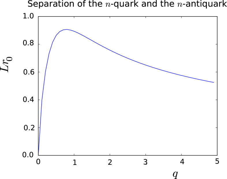
Figure 1: In this figure we plot $L\,r_{0}$ as a function of $q$, as given by (6.19). The maximal value of $L\,r_{0}$ occurs when $q\approx 0.779$. For this value of $q$ we get $L\,r_{0}\approx 0.906$.

In figure 1 we have plotted $r_{0}\,L\,=\,{4\pi\over 3}\,\,T\,L$ as a function of $q$. It is clear from this figure that there exists a maximal value of $L$ for every temperature $T$ and that for fixed $L$ there are no connected configurations for large enough temperature. Moreover, when $r_{0}\,L$ is small enough there are two possible values of $q$ which, according to (6.18), correspond to two possible values of $r_{*}$. In order to determine which of these two configurations is the dominant one, let us compute the free energy as a function of $q$. First of all, notice that plugging eq. (6.12) into the expression of the energy density given by (6.7), we get:

$${\cal H}\,=\,E_{n}\,{r^{2}\sqrt{f(r)}\over\sqrt{r^{4}\,f(r)\,-\,\hat{\Lambda}^{2}}}\,\,.$$ (6.20)

Let us integrate this energy density for a connected configuration whose ends are located at $r=r_{\max}$. One gets:

$$E\,=\,2E_{n}\,\int_{r_{*}}^{r_{max}}\,{\rho^{2}\sqrt{f(\rho)}\over\sqrt{\rho^{4}\,f(\rho)\,-\,\hat{\Lambda}^{2}}}\,d\rho\,\,.$$ (6.21)

Changing variables in (6.21) from $\rho$ to $z=\rho/r_{0}$, we get:

$$E\,=\,2E_{n}\,r_{0}\,\int_{z_{*}}^{z_{max}}\,{\sqrt{z^{4}-z}\over\sqrt{z^{4}-z-q^{2}}}\,\,dz\,\,.$$ (6.22)

This integral is divergent when $z_{max}\rightarrow\infty$. In order to regulate it and get the free energy, we follow the procedure in [22, 23] and subtract the energy corresponding to a disconnected configuration that reaches the point $r=r_{max}$. This energy is:

$$2E_{n}\int_{0}^{r_{max}}\,d\rho\,=\,2E_{n}\,r_{0}\Big{[}\,\int_{z_{*}}^{z_{max}}\,dz\,+\,z_{*}\,\Big{]}\,\,.$$ (6.23)

The regulated free energy for the connected configuration (after sending $z_{\max}\rightarrow\infty$) is given by:

$$F\,=\,2E_{n}\,r_{0}\,\Bigg{[}\,\int_{z_{*}}^{\infty}\,\Bigg{(}\,{\sqrt{z^{4}-z}\over\sqrt{z^{4}-z-q^{2}}}\,-\,1\,\Bigg{)}\,dz\,-\,z_{*}\,\Bigg{]}\,\,.$$ (6.24)

Notice that for $q=0$ (and $z_{*}=1$) the free energy in (6.24) $F=-2E_{n}\,r_{0}$, i.e. twice the result in (5.10) and (5.11), which confirms that this $q=0$ configuration corresponds to two straight disconnected branes stretching from the boundary to the horizon.

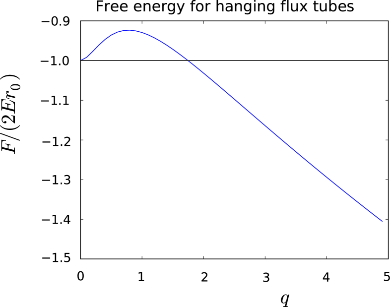
Figure 2: Plot of $F/(2E_{n}r_{0})$ as a function of the parameter $q$. The curve reaches a maximum at $q\approx 0.789$, where it takes the value $F/(2E_{n}r_{0})\approx-0.923$. The dimerization transition starts at $q\approx 1.747$, where $F=-2E_{n}\,r_{0}$.

The free energy $F$ as a function of $q$ has been plotted in figure 2. By comparing figures 1 and 2 it is easy to verify that, when $r_{0}\,L$ is small enough to allow two solutions for $q$, the configuration with higher $q$ (i.e. the one that penetrates less deeply in the bulk) is the one that has lower free energy and, therefore, is the dominant one. It is also clear from figure 2 that, for low enough temperature, this configuration has a free energy lower than $-2E_{n}\,r_{0}$ and, therefore, it is also dominant over the disconnected one. This reconnection of branes at low temperature is the dimerization transition described in [7]. Its characteristics are very similar to the ones of the ${\cal N}=4$ four-dimensional theory and will not be elaborated further here.

7 Impurity fluctuations

Let us now consider fluctuations around the static configurations studied above. We will allow to fluctuate the coordinates transverse to the D6-brane (namely the angle $\alpha$ and the cartesian coordinates $x$ and $y$), as well as the worldvolume field $F$. Thus, we write:

$$\alpha\,=\,\alpha_{n}\,+\,\xi\,\,,\qquad F\,=\,\bar{f}\,+\,f\,\,,\qquad x\,=\,\bar{x}\,+\,\chi\,\,,$$ (7.1)

where $\alpha_{n}$ is the angle determined in (4.7), $\bar{x}$ is the constant cartesian coordinate of the unperturbed D6-brane and the only non-zero component of the gauge field $\bar{f}$ is the one written in (4.10). The equations of motion for the fluctuations can be written in terms of the the open string metric (see appendix B), which takes the form:

$${\cal G}_{mn}\,d\zeta^{m}\,d\zeta^{n}\,=\,{R^{3}\over 4k}\,\,\big{[}\,\sin^{2}\alpha_{n}\,ds^{2}_{AdS_{2}}\,+\,ds^{2}_{\tilde{T}^{1,1}}\,\big{]}\,\,,$$ (7.2)

where $ds^{2}_{AdS_{2}}=-r^{2}\,dt^{2}\,+\,dr^{2}/r^{2}$ and $ds^{2}_{\tilde{T}^{1,1}}$ has been written in (4.12) and (4.14). In terms of the metric ${\cal G}_{mn}$, the total lagrangian density for the fluctuations takes the form:

$${\cal L}\,=\,-T_{6}\,\,{R^{9}\over 2^{7}\,k^{2}}\,\sin\alpha_{n}\,\sqrt{\tilde{g}}\,\Bigg{[}\,{R^{3}\over 4k}\,{1\over 2}\,r^{2}\,{\cal G}^{mn}\,\partial_{m}\,\chi\,\partial_{n}\,\chi\,+\,{R^{3}\over 4k}\,{1\over 2}\,{\cal G}^{mn}\,\partial_{m}\,\xi\,\partial_{n}\,\xi\,+\,$$

$$\qquad\qquad\qquad\qquad+{1\over 4}\,{\cal G}^{mp}\,{\cal G}^{nq}\,f_{pq}\,f_{mn}\,-\,{3\over 2}\,{\xi^{2}\over\sin^{2}\alpha_{n}}\,-\,{12k\over R^{3}}\,{\xi f_{0r}\over\sin^{3}\alpha_{n}}\,\Bigg{]}\,\,.$$ (7.3)

Let us now write the equations of motion derived from this lagrangian density for the different fluctuations. First of all, we write the one corresponding to the fluctuations $\chi$ of the cartesian coordinates, namely:

$$\partial_{m}\,\Big{[}\,r^{2}\sqrt{\tilde{g}}\,\,{\cal G}^{mn}\,\partial_{n}\,\chi\,\Big{]}\,=\,0\,\,.$$ (7.4)

The equations for the scalar $\xi$ and the gauge field are coupled. The equation for $\xi$ is:

$${R^{3}\over 4k}\,\,{1\over\sqrt{\tilde{g}}}\,\partial_{m}\,\Big{[}\sqrt{\tilde{g}}\,{\cal G}^{mn}\,\partial_{n}\xi\,\Big{]}\,+\,{3\over\sin^{2}\bar{\alpha}_{n}}\,\xi\,+\,{12k\over R^{3}}\,\,{f_{0r}\over\sin^{3}\alpha_{n}}\,=\,0\,\,,$$ (7.5)

whereas the equation for the gauge field is:

$${1\over\sqrt{\tilde{g}}}\,\partial_{m}\,\Big{[}\sqrt{\tilde{g}}\,{\cal G}^{mp}\,{\cal G}^{nq}\,f_{pq}\,\Big{]}\,+\,{12k\over R^{3}}\,\,{1\over\sin^{3}\alpha_{n}}\,\Big{[}\partial_{r}\xi\,\delta^{n}_{0}\,-\,\partial_{0}\xi\,\delta^{n}_{r}\,\Big{]}\,=\,0\,\,.$$ (7.6)

7.1 Fluctuation of the cartesian coordinates

Let us consider in detail the fluctuations $\chi$ of the cartesian coordinates. By using the expression of ${\cal G}^{mn}$ in (B.12), eq. (7.4) becomes:

$$\partial_{r}\,\big{(}\,r^{4}\,\partial_{r}\,\chi\,\big{)}\,-\,\partial_{0}^{2}\,\chi\,+\,r^{2}\,\sin^{2}\alpha_{n}\,\,\nabla^{2}_{\tilde{T}^{1,1}}\,\chi\,=\,0\,\,.$$ (7.7)

Let us separate variables in this equation as follows:

$$\chi\,=\,e^{iEt}\,Y_{l_{1},l_{2}}(\tilde{T}^{1,1})\,\phi(r)\,\,,$$ (7.8)

where $Y_{l_{1},l_{2}}(\tilde{T}^{1,1})$ are the scalar harmonic functions for the squashed $T^{1,1}$ (see appendix C), which depend, among other quantum numbers, on two integers $l_{1}$ and $l_{2}$. As shown in appendix C, the eigenvalues of the laplacian in a squashed $T^{1,1}$ space with general squashing factors depend on $l_{1}$, $l_{2}$ and on the R-charge quantum number $r$ (see (C.8)). Remarkably, for the particular squashing of (4.14) the dependence on the R-charge $r$ drops (see (C.12)). Actually, by using the eigenvalues of the laplacian derived in the appendix C, we get:

$$\sin^{2}\alpha_{n}\,\,\nabla^{2}_{\tilde{T}^{1,1}}\,Y_{l_{1},l_{2}}\,=\,-\big{[}\,l_{1}(l_{1}+2)\nu\,+\,l_{2}(l_{2}+2)\,(1-\nu)\,\big{]}\,Y_{l_{1},l_{2}}\,\,,$$ (7.9)

with $\nu$ being the filling fraction ($\nu=n/N$). Using this result, the equation for the radial function $\phi(r)$ becomes:

$$\partial_{r}\,\big{(}\,r^{4}\,\partial_{r}\,\phi\,\big{)}\,+\,E^{2}\,\phi\,-\,r^{2}\,\big{[}\,l_{1}(l_{1}+2)\nu\,+\,l_{2}(l_{2}+2)\,(1-\nu)\,\big{]}\,\phi\,=\,0\,\,.$$ (7.10)

Let us now study the behavior of the solutions of this equation for large $r$. We assume that $\phi\sim r^{\alpha}$ for large $r$. By keeping only the leading terms we get that $\alpha$ must satisfy the following quadratic equation:

$$\alpha(\alpha+3)\,=\,l_{1}(l_{1}+2)\nu\,+\,l_{2}(l_{2}+2)\,(1-\nu)\,\,,$$ (7.11)

which has two solutions, namely:

$$\alpha_{\pm}\,=\,-{3\over 2}\,\pm\,\sqrt{\Big{(}{3\over 2}\Big{)}^{2}\,+\,l_{1}(l_{1}+2)\nu\,+\,l_{2}(l_{2}+2)\,(1-\nu)}\,\,.$$ (7.12)

Thus, at large $r$, the fluctuation $\phi$ becomes:

$$\phi(r)\sim\,c_{+}\,r^{\alpha_{+}}\,+\,c_{-}\,r^{\alpha_{-}}\,\,.$$ (7.13)

In general, in $AdS_{2}$, if a fluctuation behaves in the UV as:

$$\chi\sim c_{1}\,r^{-2a_{1}}\,+\,c_{2}\,r^{-2a_{2}}\,\,,\qquad\qquad a_{2}>a_{1}\,\,,$$ (7.14)

then, the dimension of the operator dual to the normalizable mode is:

$$\Delta\,=\,{1\over 2}\,+\,a_{2}-a_{1}\,\,.$$ (7.15)

In our case:

$$a_{1}\,=\,-{\alpha_{+}\over 2}\,\,,\qquad\qquad a_{2}\,=\,-{\alpha_{-}\over 2}\,\,,$$ (7.16)

and, therefore, the conformal dimension $\Delta$ is just:

$$\Delta\,=\,{1\over 2}\,+\,\sqrt{\Big{(}{3\over 2}\Big{)}^{2}\,+\,l_{1}(l_{1}+2)\nu\,+\,l_{2}(l_{2}+2)\,(1-\nu)}\,\,.$$ (7.17)

Notice that $\Delta=2$ for $l_{1}=l_{2}=0$ and, that in general the dimensions are not rational numbers. This is, actually, what happens for the supergravity backgrounds that contain the $T^{1,1}$ space (i.e. the conifold-like theories). Moreover, the dimensions depend on the filling fraction $\nu$. Only in the symmetric representations in which $l_{1}=l_{2}=l$ this dependence on $\nu$ disappears. Indeed, in this case one gets the simple formula:

$$\Delta\,=\,{1\over 2}\,+\,\sqrt{\Big{(}{3\over 2}\Big{)}^{2}\,+\,l(l+2)}\,\,,\qquad\qquad(l_{1}=l_{2}=l).$$ (7.18)

7.2 Coupled modes

Let us now consider a solution of the equations of motion of the fluctuations in which the gauge field components $a_{r}$ and $a_{i}$ are non-zero and given by the ansatz:

$$a_{r}\,=\,e^{iEt}\,Y_{l_{1},l_{2}}(\tilde{T}^{1,1})\,\phi(r)\,\,,\qquad\qquad a_{i}\,=\,e^{iEt}\,\nabla_{i}Y_{l_{1},l_{2}}(\tilde{T}^{1,1})\tilde{\phi}(r)\,\,.$$ (7.19)

In addition, we will adopt the ansatz in which the scalar field $\xi$ is also fluctuating and given by:

$$\xi\,=\,e^{iEt}\,Y_{l_{1},l_{2}}(\tilde{T}^{1,1})\,z(r)\,\,.$$ (7.20)

For this ansatz of the gauge potential, the non-vanishing components of the gauge field strength $f=da$ are:

$$f_{0r}\,=\,iE\,a_{r}\,\,,\qquad f_{0i}\,=\,iE\,a_{i}\,\,,\qquad f_{ri}\,=\,e^{iEt}\,(\partial_{r}\tilde{\phi}-\phi)\,\nabla_{i}\,Y_{l_{1},l_{2}}(\tilde{T}^{1,1})\,\,.\qquad$$ (7.21)

We can now write the different components of the coupled equations of motion (7.5) and (7.6). The equation of motion (7.6) for the gauge field for the index $n=0$ is:

$$c_{l_{1},l_{2}}^{\nu}\,\tilde{\phi}\,=\,r^{2}\,\partial_{r}\,\phi\,-\,{3i\over E}\,\,{R^{3}\over 4k}\,r^{2}\,\sin\alpha_{n}\,\partial_{r}\,z\,\,.$$ (7.22)

where $c_{l_{1},l_{2}}^{\nu}$ is the eigenvalue of $\sin^{2}\alpha_{n}\,\,\nabla^{2}_{\tilde{T}^{1,1}}\,Y_{l_{1},l_{2}}$ (see (7.9)), namely:

$$c_{l_{1},l_{2}}^{\nu}\,\equiv\,l_{1}(l_{1}+2)\nu\,+\,l_{2}(l_{2}+2)\,(1-\nu)\,\,.$$ (7.23)

For the index $n=r$ the gauge field equation (7.6) gives:

$$E^{2}\,\phi\,+\,c_{l_{1},l_{2}}^{\nu}\,r^{2}\,(\partial_{r}\tilde{\phi}-\phi)\,-\,{3R^{3}\over 4k}\,\sin\alpha_{n}\,iE\,z\,=\,0\,\,.$$ (7.24)

Finally, for $n=i$ we get the following relation between $\tilde{\phi}$ and $\phi$:

$$E^{2}\,\tilde{\phi}\,=\,-r^{2}\,\partial_{r}\,\big{[}\,r^{2}\,(\partial_{r}\,\tilde{\phi}\,-\,\phi)\,\big{]}\,\,.$$ (7.25)

One can verify that this last equation (7.25) is a consequence of (7.22) and (7.24). Moreover, we can use (7.22) to eliminate $\tilde{\phi}$ from the equations of motion of the gauge field. The resulting equation for $\phi$ is:

$$\partial_{r}\,(r^{2}\partial_{r}\phi)\,+\,{E^{2}\over r^{2}}\,\phi\,-\,c_{l_{1},l_{2}}^{\nu}\,\phi\,-\,{3i\over E}\,{R^{2}\over 4k}\,\sin\alpha_{n}\,\big{[}\partial_{r}\,(r^{2}\partial_{r}\,z)\,+\,{E^{2}\over r^{2}}\,z\,\big{]}\,=\,0\,\,.$$ (7.26)

The equation of motion (7.5) for the scalar $\xi$ becomes:

$$\partial_{r}\,(r^{2}\partial_{r}\,z)\,+\,{E^{2}\over r^{2}}\,z\,+\,(\,3\,-\,c_{l_{1},l_{2}}^{\nu}\,)\,z\,+\,{3iE\over\sin\alpha_{n}}\,{4k\over R^{3}}\,\phi\,=\,0\,\,.$$ (7.27)

Let us now decouple the two equations (7.26) and (7.27). First of all, we define the differential operator $\hat{\cal O}$ as the one that acts on an arbitrary function $\psi$ as:

$$\hat{\cal O}\,\psi\,\equiv\,\partial_{r}\,(r^{2}\partial_{r}\,\psi)\,+\,{E^{2}\over r^{2}}\,\psi\,\,.$$ (7.28)

Next, we define the functions $\hat{z}$ and $\eta$ as:

$$\hat{z}\,=\,-{i\over E}\,{R^{3}\over 4k}\,\,\sin\alpha_{n}\,z\,\,,\qquad\qquad\eta\,=\,\phi\,-\,{3i\over E}\,{R^{3}\over 4k}\,\sin\alpha_{n}\,z\,\,.$$ (7.29)

Then, one can show that (7.26) and (7.27) can be written as the following matrix equation:

$$\Big{(}\,\,\hat{\cal O}\,-\,{\cal M}\,\,\Big{)}\,\left(\begin{array}[]{c}\,\hat{z}\\ \eta\end{array}\right)=\,0\,\,,$$ (7.30)

where ${\cal M}$ is the following $2\times 2$ matrix:

$${\cal M}\,=\,\left(\begin{array}[]{ccc}c_{l_{1},l_{2}}^{\nu}+6&&-3\\ \\ \\ -3c_{l_{1},l_{2}}^{\nu}&&c_{l_{1},l_{2}}^{\nu}\end{array}\right)\,\,.$$ (7.31)

In what follows we will distinguish the case in which $c_{l_{1},l_{2}}^{\nu}\not=0$ from the case in which it vanishes and the fluctuation is an s-wave in the internal $\tilde{T}^{1,1}$ space with $l_{1}=l_{2}=0$. Actually, it follows from (7.22) and (7.24) that $\eta=0$ when $c_{l_{1},l_{2}}^{\nu}=0$ and, therefore, in this case there is only one type of mode, namely that corresponding to $\hat{z}$. Notice that (7.30) is consistent with having $\eta=0$ when $c_{l_{1},l_{2}}^{\nu}=0$.

Let us consider from now on the case $c_{l_{1},l_{2}}^{\nu}\not=0$. In this case we have to deal with the full matrix equation (7.30). The matrix ${\cal M}$ written above is diagonalizable and its two eigenvalues are:

$$\lambda_{l_{1},l_{2}}^{(\pm)}\,=\,c_{l_{1},l_{2}}^{\nu}\,+\,3\,\big{(}\,1\,\pm\sqrt{1+c_{l_{1},l_{2}}^{\nu}}\,\big{)}\,\,.$$ (7.32)

The corresponding eigenfunctions are the following combinations of $\hat{z}$ and $\eta$:

$$\psi_{\pm}\,=\,\big{(}\,\sqrt{1+c_{l_{1},l_{2}}^{\nu}}\,\pm 1\,\big{)}\,\hat{z}\,\mp\,\eta\,\,.$$ (7.33)

Indeed, one can check that $\psi_{\pm}$ satisfy the following decoupled equations:

$$\partial_{r}\,(r^{2}\partial_{r}\,\psi_{\pm})\,+\,\Big{(}\,{E^{2}\over r^{2}}\,-\,\lambda_{l_{1},l_{2}}^{(\pm)}\,\Big{)}\,\psi_{\pm}\,=\,0\,\,.$$ (7.34)

In order to obtain the conformal dimensions associated to the normalizable solutions of (7.34), let us study the behavior of the functions $\psi_{\pm}(r)$ for large $r$. By considering functions of the type $\psi_{\pm}(r)\sim r^{a}$, one gets two possible solutions for $a$ and, thus, $\psi_{\pm}(r)$ behaves for large $r$ as:

$$\psi_{\pm}(r)\sim c_{1}\,r^{-2a_{1}^{(\pm)}}\,+\,c_{2}\,r^{-2a_{2}^{(\pm)}}\,\,,$$ (7.35)

where $c_{1}$ and $c_{2}$ are constants and the exponents $a_{1}^{(\pm)}$ and $a_{2}^{(\pm)}$ are given by:

$$a_{1}^{(\pm)}\,=\,{1-\sqrt{1+4\,\lambda_{l_{1},l_{2}}^{(\pm)}}\over 4}\,\,,\qquad\qquad a_{2}^{(\pm)}\,=\,{1+\sqrt{1+4\,\lambda_{l_{1},l_{2}}^{(\pm)}}\over 4}\,\,.$$ (7.36)

The conformal dimensions $\Delta_{\pm}$ of the operators dual to the normalizable modes of $\psi_{\pm}(r)$ are immediately obtained from the general equation (7.15):

$$\Delta_{\pm}\,=\,{1\over 2}\,\,\Big{(}\,1\,+\,\sqrt{1+4\,\lambda_{l_{1},l_{2}}^{(\pm)}}\,\Big{)}\,\,.$$ (7.37)

Remarkably, $1+4\,\lambda_{l_{1},l_{2}}^{(\pm)}$ is a perfect square. Indeed, by using (7.32) one can straightforwardly prove that:

$$1+4\,\lambda_{l_{1},l_{2}}^{(\pm)}\,=\,\Big{(}\,2\,\sqrt{1+c_{l_{1},l_{2}}^{\nu}}\pm 3\,\Big{)}^{2}\,\,.$$ (7.38)

Therefore, the conformal dimensions $\Delta_{\pm}$ can be simply be written as:

$$\Delta_{+}\,=\,2\,+\,\sqrt{1+c_{l_{1},l_{2}}^{\nu}}\,\,,\qquad\qquad\Delta_{-}\,=\,\sqrt{1+c_{l_{1},l_{2}}^{\nu}}\,-\,1\,\,.$$ (7.39)

Recall that, to obtain (7.39), we have assumed that $c_{l_{1},l_{2}}^{\nu}>0$, which ensures that $\Delta_{-}>0$. When $c_{l_{1},l_{2}}^{\nu}$ vanishes then $\eta=0$ and the matrix equation (7.30) reduces to the simple equation $\big{(}\,\hat{\cal O}\,-\,6\,\big{)}\,\hat{z}\,=\,0$. It is then straightforward to demonstrate that the normalizable mode has conformal dimension $\Delta=3$, which is the same value as the one that is obtained by substituting $c_{l_{1},l_{2}}^{\nu}=0$ in the equation giving $\Delta_{+}$ in (7.39).

The dimensions (7.39) are, in general, not rational and they depend on the filling fraction $\nu$. However, for symmetric representations in which $l_{1}=l_{2}=l$ the dependence on $\nu$ disappears and one has:

$$c_{l,l}^{\nu}\,=\,l(l+2)\,\,\Longrightarrow\sqrt{1+c_{l,l}^{\nu}}\,=\,l+1\,\,.$$ (7.40)

Therefore, in this symmetric case the dimensions are rational and are given by:

$$\Delta_{+}\,=\,3\,+l\,\,,\qquad(l\geq 0)\,\,,\qquad\qquad\Delta_{-}\,=\,l\,\,,\qquad(l>0)\,\,,$$ (7.41)

where we have already taken into account the $l=0$ case.

7.3 Internal gauge field modes

We now consider fluctuation modes of the gauge field in which the only components which are non-vanishing are those along the directions of the internal $\tilde{T}^{1,1}$ space (they will be denoted by $a_{i}$). In this case the non-zero components of the field strength $f$ are:

$$f_{0i}\,=\,\partial_{0}\,a_{i}\,\,,\qquad\qquad f_{ri}\,=\,\partial_{r}\,a_{i}\,\,,\qquad\qquad f_{ij}\,=\,\partial_{i}\,a_{j}\,-\,\partial_{j}\,a_{i}\,\,.$$ (7.42)

The equations of motion (7.6) for the gauge field for $n=0,r$ are just:

$$\partial_{0}\big{(}\,\nabla^{i}\,a_{i}\,\big{)}\,=\,0\,\,,\qquad\qquad\partial_{r}\big{(}\,\nabla^{i}\,a_{i}\,\big{)}\,=\,0\,\,,$$ (7.43)

where:

$$\nabla^{i}\,a_{i}\,=\,{1\over\sqrt{\tilde{g}}}\,\partial_{i}\,\big{(}\,\sqrt{\tilde{g}}\,\tilde{g}^{ij}\,a_{j}\,\big{)}\,\,.$$ (7.44)

Thus, clearly we should require the fulfillment of the following transversality condition:

$$\nabla^{i}\,a_{i}\,=\,0\,\,.$$ (7.45)

We now write the equation (7.6) for $n=i$, namely:

$$\tilde{g}^{ij}\,\Big{[}\,\partial_{r}\,\big{[}\,r^{2}\,\partial_{r}\,a_{j}\,\big{]}\,-\,\,r^{-2}\,\partial_{0}^{2}\,a_{j}\,\Big{]}\,+\,{\sin^{2}\alpha_{n}\over\sqrt{\tilde{g}}}\,\partial_{k}\,\big{[}\sqrt{\tilde{g}}\,(\partial^{k}a^{i}-\partial^{i}a^{k}\,)\,\big{]}\,=\,0\,\,.$$ (7.46)

The last term in this equation can be rewritten as:

$${1\over\sqrt{\tilde{g}}}\,\partial_{k}\,\big{[}\sqrt{\tilde{g}}\,(\partial^{k}a^{i}-\partial^{i}a^{k}\,)\,\big{]}\,=\,\nabla_{k}\nabla^{k}\,a^{i}\,-\,R^{i}_{\,\,k}\,a^{k}\,-\,\nabla^{i}\,\nabla_{k}\,a^{k}\,\,,$$ (7.47)

where $R^{i}_{\,\,k}$ is the Ricci tensor of the $\tilde{T}^{1,1}$ space. Taking (7.45) into account, the last term in (7.47) vanishes and the right-hand side of (7.47) can be written in terms of the Hodge-de Rham operator $\Delta_{1}$, which acts on a vector field with components $f_{i}$ as:

$$\Delta_{1}\,f_{i}\,\equiv\,-\nabla_{k}\nabla^{k}\,f_{i}\,+\,R^{k}_{i}\,f_{k}\,\,.$$ (7.48)

Thus, the equation of motion (7.46) becomes:

$$\partial_{r}\,\big{[}\,r^{2}\,\partial_{r}\,a_{i}\,\big{]}\,-\,\,{1\over r^{2}}\,\partial_{0}^{2}\,a_{i}\,-\,4\nu\,(1-\nu)\,\Delta_{1}\,a_{i}\,=\,0\,\,,$$ (7.49)

where we have taken into account that $\sin^{2}\alpha_{n}\,=\,4\nu\,(1-\nu)$. Let us next separate variables in $a_{i}$ as:

$$a_{i}\,=\,e^{iEt}\,Y_{i}(\tilde{T}^{1,1})\,\phi(r)\,\,,$$ (7.50)

where $Y_{i}(\tilde{T}^{1,1})$ is a vector spherical harmonic for the $\tilde{T}^{1,1}$ space which satisfies the transversality condition:

$$\nabla^{i}\,Y_{i}(\tilde{T}^{1,1})\,=\,0\,\,.$$ (7.51)

Let us diagonalize the Hodge-de Rham operator $\Delta_{1}$ in the space of the $\tilde{T}^{1,1}$ vector harmonics and write:

$$4\nu\,(1-\nu)\,\Delta_{1}\,Y_{i}\,=\,\Lambda\,Y_{i}\,\,,$$ (7.52)

where the eigenvalue $\Lambda$ will depend on the quantum numbers $l_{1}$ and $l_{2}$, as well as on the filling fraction $\nu$ (see below). By plugging the ansatz (7.50) on the fluctuation equation (7.49), one gets the following equation for the radial function $\phi(r)$:

$$\partial_{r}\,\big{[}\,r^{2}\,\partial_{r}\,\phi\,\big{]}\,+\,{E^{2}\over r^{2}}\,\phi\,-\,\Lambda\,\phi\,=\,0\,\,.$$ (7.53)

This equation can be solved for large $r$ by taking $\phi\sim r^{\alpha}$, with $\alpha$ being some exponent. Taking into account that the term with the energy is subleading at large $r$, one gets that the exponent $\alpha$ must satisfy the following quadratic equation:

$$\alpha\,(\alpha+1\,)\,=\,\Lambda\,\,,$$ (7.54)

which has two solutions, namely:

$$\alpha_{\pm}\,=\,{-1\pm\sqrt{1+4\Lambda}\over 2}\,\,.$$ (7.55)

Thus, $\phi(r)$ behaves as (7.14) with $a_{1}=-\alpha_{+}/2$ and $a_{2}=-\alpha_{-}/2$, i.e. as in (7.16). Therefore, the conformal dimension of the operator dual to these fluctuations is:

$$\Delta\,=\,{1\over 2}\,\,\Big{(}\,1\,+\,\sqrt{1+4\Lambda}\,\Big{)}\,\,.$$ (7.56)

Let us analyze the different dimensions obtained for the various vector harmonics for the $\tilde{T}^{1,1}$ space that were studied in appendix D. As shown in this appendix, the results depend on whether the filling fraction $\nu$ is arbitrary or $\nu=1/2$. These two cases will be studied separately in what follows.

7.3.1 Arbitrary filling

As argued in appendix D in this case we should take vanishing R-charge $r$ and the eigenvalues $\Lambda$ depend on the remaining two quantum numbers $l_{1}$ and $l_{2}$. Actually, there are two series of eigenvalues, which were denoted by $\lambda_{1}$ and $\lambda_{2}$ in the appendix. Let us consider the first of these modes and let us denote by $\Lambda_{1}$ the corresponding value of $\Lambda$ in (7.52). From the value of $\lambda_{1}$ written in (D.28), we get:

$$\Lambda_{1}\,=\,c_{l_{1},l_{2}}^{\nu}\,\,.$$ (7.57)

The associated conformal dimension $\Delta_{1}$ is given by:

$$\Delta_{1}\,=\,{1\over 2}\,\,\Big{(}\,1\,+\,\sqrt{1+4\,c_{l_{1},l_{2}}^{\nu}}\,\Big{)}\,\,,$$ (7.58)

which is, in general, not rational. Moreover, only for $l_{1}=l_{2}=l$ the dimension $\Delta_{1}$ is independent of the filling fraction since $c^{\nu}_{l,l}=l(l+1)$.

The second class of eigenvalues in this arbitrary filling case, denoted by $\lambda_{2}^{(\pm)}$ in (D.28), lead to a value of $\Lambda$ given by:

$$\Lambda_{2}^{(\pm)}\,=\,1\,+\,c_{l_{1},l_{2}}^{\nu}\pm\sqrt{1+4\nu^{3}\,l_{1}(l_{1}+2)\,+\,4(1-\nu)^{3}\,l_{2}(l_{2}+2)}\,\,.$$ (7.59)

The corresponding conformal dimension is:

$$\Delta_{2}^{(\pm)}\,=\,{1\over 2}\,+\,\sqrt{{5\over 4}\,+\,c_{l_{1},l_{2}}^{\nu}\pm\sqrt{1+4\nu^{3}\,l_{1}(l_{1}+2)\,+\,4(1-\nu)^{3}\,l_{2}(l_{2}+2)}}\,\,.$$ (7.60)

We will see below that this formula simplifies greatly if $\nu=1/2$.

7.3.2 Half filling

When $\nu=1/2$, it was shown in appendix D that there are transverse modes for $r\not=0$. As in the generic $\nu$ case, there are two types of modes. The eigenvalues of the first type were denoted by $\tilde{\lambda}_{1}$ in (D.29) and they lead to the following eigenvalue in (7.52):

$$\tilde{\Lambda}_{1}^{\pm}\,=\,\tilde{c}_{l_{1},l_{2}}\pm r\,\,,$$ (7.61)

with $\tilde{c}_{l_{1},l_{2}}$ being the value of $c_{l_{1},l_{2}}^{\nu}$ for $\nu=1/2$, i.e.:

$$\tilde{c}_{l_{1},l_{2}}\,\equiv\,c_{l_{1},l_{2}}^{\nu=1/2}\,=\,{l_{1}(l_{1}+2)\over 2}\,+\,{l_{1}(l_{1}+2)\over 2}\,\,.$$ (7.62)

The dimension of these modes are non-rational and given by:

$$\tilde{\Delta}_{1}^{(\pm)}\,=\,{1\over 2}\,+\,\sqrt{{1\over 4}\,+\,\tilde{c}_{l_{1},l_{2}}\pm r}\,\,.$$ (7.63)

For $r=0$ these dimensions reduce to the ones written in (7.58) for $\nu=1/2$.

Next, let us consider the modes with eigenvalues $\tilde{\lambda}_{2}^{(\pm)}$, for which the eigenvalue defined in (7.52) is independent of $r$ and given by:

$$\tilde{\Lambda}_{2}^{(\pm)}\,=\,1\,+\,\tilde{c}_{l_{1},l_{2}}\pm\sqrt{1+\tilde{c}_{l_{1},l_{2}}}\,\,.$$ (7.64)

Remarkably, one can verify that $1+4\,\tilde{\Lambda}_{2}^{(\pm)}$ can be written as a square. Indeed, one can straightforwardly check that:

$$1+4\,\tilde{\Lambda}_{2}^{(\pm)}\,=\,\Big{(}\,2\,\sqrt{1+\tilde{c}_{l_{1},l_{2}}}\pm 1\,\Big{)}^{2}\,\,.$$ (7.65)

Thus, the associated conformal dimensions $\tilde{\Delta}_{2}^{(+)}$ and $\tilde{\Delta}_{2}^{(-)}$ are just:

$$\tilde{\Delta}_{2}^{(+)}\,=\,1\,+\,\sqrt{1+\tilde{c}_{l_{1},l_{2}}}\,\,,\qquad\qquad\tilde{\Delta}_{2}^{(-)}\,=\,\sqrt{1+\tilde{c}_{l_{1},l_{2}}}\,\,.$$ (7.66)

These dimensions are generically not rational. However, when $l_{1}=l_{2}=l$, one has that $\sqrt{c}_{l,l}=l(l+2)$ and, thus, $\sqrt{1+c_{l,l}}=l+1$. Therefore, in this $l_{1}=l_{2}=l$ case the dimensions associated to these modes are rational and given by:

$$\tilde{\Delta}_{2}^{(+)}\,=\,2+l\,\,,\qquad\qquad\tilde{\Delta}_{2}^{(-)}\,=\,1+l\,\,,\qquad\qquad(l_{1}=l_{2}=l)\,\,.$$ (7.67)

8 Dimer fluctuations

Let us now consider the fluctuations around a connected configuration of the type studied in section 6. We will restrict ourselves to analyze the case in which the background is supersymmetric, i.e. for vanishing temperature. Recall that in this case the D6-branes do not reach the origin at $r=0$ and they extend along the Minkowski directions (say, along the coordinate $x$). For this reason we will have to distinguish between longitudinal and transverse fluctuations in the $(x,y)$ plane. By computing the lagrangian for generic quadratic fluctuations one realizes that most of the modes are coupled and the diagonalization of the equations of motion is rather involved. However, one can verify that the fluctuation of the transverse position in the Minkowski space is decoupled from the other modes. In this paper we will limit ourselves to studying these transverse fluctuations. The corresponding lagrangian density and equation of motion are derived in appendix B (eqs. (B.37) and (B.38), respectively). More explicitly, the equation of motion for the transverse modes can be written as:

$$\partial_{r}\,\big{(}\,r^{2}\,\sqrt{r^{4}-r_{*}^{4}}\,\,\partial_{r}\,\chi\,\big{)}\,-\,{r^{2}\over\sqrt{r^{4}-r_{*}^{4}}}\,\partial_{0}^{2}\,\chi\,+\,{r^{4}\over\sqrt{r^{4}-r_{*}^{4}}}\,\sin^{2}\alpha_{n}\,\,\nabla^{2}_{\tilde{T}^{1,1}}\,\chi\,=\,0\,\,,$$ (8.1)

where $r_{*}$ is the minimal value of the $r$ coordinate attained by the unperturbed configuration of the brane. Notice also that any value of $r$ in the interval $[r_{*},+\infty)$ is reached twice by the brane.

Let us separate variables in (8.1) as in (7.8) and let us define the rescaled radial coordinate $\rho$ and the rescaled energy $\bar{E}$ as:

$$\rho\,=\,{r\over r_{*}}\,\,,\qquad\qquad\bar{E}\,=\,{E\over r_{*}}\,\,.$$ (8.2)

In terms of these quantities, the equation of motion for the fluctuation becomes:

$$\partial_{\rho}\,\big{(}\,\rho^{2}\,\sqrt{\rho^{4}-1}\,\,\partial_{\rho}\,\phi\,\big{)}\,+\,\bar{E}^{2}\,{\rho^{2}\over\sqrt{\rho^{4}-1}}\,\phi\,-\,c_{l_{1},l_{2}}^{\nu}{\rho^{4}\over\sqrt{\rho^{4}-1}}\,\phi\,=\,0\,\,,$$ (8.3)

where $c_{l_{1},l_{2}}^{\nu}$ has been defined in (7.23).

When $c_{l_{1},l_{2}}^{\nu}=0$ (or equivalently for the s-wave modes with $l_{1}=l_{2}=0$), the fluctuation equation (8.3) can be exactly solved by means of a change of variables found in [24, 25]. Indeed, let us introduce a new variable $\eta$, related to $\rho$ by means of the equation:

$$\eta\,=\,\int_{1}^{\rho}\,{d\bar{\rho}\over(\bar{\rho}^{2}+\bar{E}^{2})\sqrt{\bar{\rho}^{4}-1}}\,\,.$$ (8.4)

By this change of variables $\rho\in[1,+\infty]$ is mapped into $\eta\in[0,\bar{\eta}(\bar{E})\,]$, where $\bar{\eta}(\bar{E})$ is defined as:

$$\bar{\eta}(\bar{E})\,\equiv\,\int_{1}^{\infty}\,{d\bar{\rho}\over(\bar{\rho}^{2}+\bar{E}^{2})\sqrt{\bar{\rho}^{4}-1}}\,\,.$$ (8.5)

Next, we introduce a new function $\Phi(\eta)$ as follows:

$$\Phi(\eta)\,=\,{\rho\over\sqrt{\rho^{2}+\bar{E}^{2}}}\,\phi(\rho)\,\,.$$ (8.6)

By explicit calculation one can prove that the equation satisfied by $\Phi(\eta)$ is simply:

$${d^{2}\Phi\over d\eta^{2}}\,+\,{1\over 4}\,\bar{E}^{2}\,(\bar{E}^{4}-1)\,\Phi\,=\,0\,\,,$$ (8.7)

which can be immediately integrated in terms of trigonometric functions. By imposing that $\Phi$ vanishes at $\eta=0,\bar{\eta}(\bar{E})$, we get the following quantization condition on the energy $\bar{E}$:

$$\bar{E}\,\sqrt{\bar{E}^{4}-1}\,\,\bar{\eta}(\bar{E})\,=\,n\pi\,\,,\qquad\qquad n=1,2,\cdots\,.$$ (8.8)

This equation must be solved numerically in order to get the energy levels.

Let us come back to the analysis of the equation (8.3) for general values of the Kaluza-Klein quantum numbers $l_{1}$ and $l_{2}$. We will show that this equation can be mapped to the Schrödinger equation of a quantum integrable model, namely the so-called Inozemtsev $BC_{1}$ model. The first step to prove this result is changing the radial variable $\rho$ by a new variable $z$, defined as:

$$z\,=\,1-\rho^{2}\,\,.$$ (8.9)

Then, one can check that the fluctuation equation (8.3) can be written as:

$${d^{2}\phi\over dz^{2}}\,+\,{1\over 2}\,\,\Big{[}\,{1\over z}\,+\,{3\over z-1}\,+\,{1\over z-2}\,\Big{]}\,\partial_{z}\,\phi\,-\,{1\over 4}\,\,{c_{l_{1},l_{2}}^{\nu}(z-1)\,+\,\bar{E}^{2}\over z(z-1)(z-2)}\,\phi\,=\,0\,\,.$$ (8.10)

This equation is a Heun’s equation, whose more general expression is given in appendix E (eq. (E.1)). As reviewed in appendix E, the Heun equation is an ordinary differential equation with four regular singular points whose location and characteristic exponents are parametrized by several numbers, which we denoted by $\alpha$, $\beta$, $\gamma$, $\delta$, $\epsilon$, $q$ and $d$ (see (E.1)). The solution of the general Heun equation (E.1) which is regular at $z=0$ is denoted $Hl(d,q;\alpha,\beta,\gamma,\delta;z)$.

By direct comparison of (8.10) and (E.1), one gets that in our case $d=2$ and that the coefficients $\gamma$, $\delta$, $\epsilon$ and $q$ are:

$$\gamma\,=\,{1\over 2}\,\,,\qquad\qquad\delta\,=\,{3\over 2}\,\,,\qquad\qquad\epsilon\,=\,{1\over 2}\,\,\qquad\qquad q\,=\,-{c_{l_{1},l_{2}}^{\nu}\over 4}\,+\,{\bar{E}^{2}\over 4}\,\,.$$ (8.11)

Notice also that the remaining parameters $\alpha$ and $\beta$ should satisfy (see (E.2)):

$$\alpha\,+\,\beta\,=\,\gamma+\delta\,+\,\epsilon\,-\,1\,=\,{3\over 2}\,\,,\qquad\qquad\alpha\beta\,=-\,{c_{l_{1},l_{2}}^{\nu}\over 4}\,\,.$$ (8.12)

In order to determine $\alpha$ and $\beta$ we use the fact that that they are the roots of the quadratic equation:

$$x^{2}\,-\,(\alpha+\beta)\,x\,+\alpha\beta\,=\,x^{2}\,-\,{3\over 2}\,x\,-\,{c_{l_{1},l_{2}}^{\nu}\over 4}\,=0\,\,,$$ (8.13)

which are:

$$\alpha\,=\,{\Delta+1\over 2}\,\,,\qquad\qquad\beta\,=\,{2-\Delta\over 2}\,\,,$$ (8.14)

with $\Delta$ being the conformal dimension (7.17). Then, the solution of the fluctuation equation which is regular at $\rho=1$ is:

$$\phi(\rho)\,=\,Hl\big{(}2,{\bar{E}^{2}+(\Delta+1)(2-\Delta)\over 4};{\Delta+1\over 2},{2-\Delta\over 2},{1\over 2},{3\over 2};1-\rho^{2}\big{)}\,\,.$$ (8.15)

When $\bar{E}=0$ we can rewrite this result in terms of a hypergeometric function (see (E.3)), namely:

$$\phi(\rho)\big{|}_{\bar{E}=0}\,=\,F\big{(}\,{\Delta+1\over 4}\,,\,{2-\Delta\over 4}\,,\,{1\over 2}\,;\,1-\rho^{4}\,\big{)}\,\,.$$ (8.16)

As reviewed in appendix E, with an additional change of variable, the Heun equation can be converted into a Schrödinger equation for a particle moving under the influence of a potential which is a combination of elliptic functions. For a generic Heun equation this potential was written in eq. (E.18). For our particular case of (8.10) the hamiltonian takes the form:

$$H\,=\,-{d^{2}\over dx^{2}}\,+\,\Delta(\Delta-1)\,\,\wp(x)\,\,,$$ (8.17)

where $\wp(x)$ is the Weierstrass function for periods $(2\omega_{1},2\omega_{3})=(1,i)$ (see eq. (E.6) for its general definition). The relation between the variable $x$ in (8.17) and the coordinate $z$ of the Heun equation has been written in (E.25). It is interesting to write here the relation between our original radial variable $r$ and the new variable $x$. One gets:

$$r\,=\,{L\,r_{*}^{2}\over\pi}\,\,\sqrt{\wp(x)}\,\,,$$ (8.18)

where $L$ is the length of the dimer (see eq. (B.32)). By means of this change of variable the equation for the fluctuation can be written as:

$$H\,\phi\,=\,{\cal E}\,\phi\,\,,$$ (8.19)

where $\phi$ is the same function as in (8.10) but now considered as a function of $x$. Moreover, the energy ${\cal E}$ of the Schrödinger problem (8.19) is related to the energy $\bar{E}$. Indeed, by using (E.21) one gets:

$$\bar{E}^{2}\,=\,{8\pi\over\Big{[}\,\Gamma\big{(}{1\over 4}\big{)}\Big{]}^{2}}\,\,{\cal E}\,\,.$$ (8.20)

Notice that the Schrödinger equation (8.19) for the hamiltonian (8.17) is nothing but the Lamé equation. When $\Delta\in{\mathbb{Z}}$ the eigenfunctions and band structure of the Lamé equation have been obtained long ago [26]. Notice, however, that in our case $\Delta\in{\mathbb{Z}}$ only when $l_{1}=l_{2}=0$ (see (7.17)).

The coordinate $x$ in (8.17) takes values in the interval $[0,1]$, where the Weierstrass function $\wp(x)$ with periods $(2\omega_{1},2\omega_{3})=(1,i)$ is real and positive and has a minimum at $x=1/2$. Moreover, $\wp(x)\rightarrow+\infty$ when $x\rightarrow 0,1$, which means that the eigenvalue problem has a discrete spectrum consisting of an infinite tower of eigenvalues. Although many results are known for these type of integrable models, we will leave this analysis for a future work and here we will content ourselves with estimating the eigenvalues by means of the WKB method. Actually, this estimate can be performed directly in the variables of eq. (8.1). Indeed, by using the equations written in [27], we get that the energy levels can be estimated as:

$$\bar{E}_{n}\,\simeq\,{\pi\over\zeta}\,\,\sqrt{\big{(}\,n+1\,\big{)}\,\big{(}\,n+\,\Delta\,)}\,\,,\qquad\qquad(n\geq 0)\,\,,$$ (8.21)

where $\zeta$ is given by the following integral:

$$\zeta\,=\,\int_{1}^{\infty}\,\,{d\rho\over\sqrt{\rho^{4}-1}}\,=\,{1\over 4\sqrt{2\pi}}\,\Big{[}\,\Gamma\big{(}{1\over 4}\big{)}\Big{]}^{2}\,\,.$$ (8.22)

Let us write this result in terms of the length $L$ of the dimer. The relation between $L$ and $r_{*}$ was written in eq. (B.32). By using this result, one finds that the un-rescaled energies $E_{n}$ are given by:

$$E_{n}\,\simeq\,{16\pi^{3}\over\big{[}\,\Gamma\big{(}{1\over 4}\big{)}\big{]}^{4}\,L}\,\,\sqrt{\big{(}\,n+1\,\big{)}\,\big{(}\,n+\,\Delta\,)}\,\,,\qquad\qquad(n\geq 0)\,\,.$$ (8.23)

9 Summary and conclusions

Let us briefly recapitulate the main content of this work. We have studied the addition of localized fermionic impurities to the ABJM Chern-Simons-matter model in 2+1 dimensions. In the holographic approach the impurities are added by means of D6-branes extended along the holographic coordinate and wrapping a squashed $T^{1,1}$ space at a fixed point of the Minkowski spacetime. The coupling of the D6-brane to the RR field of the background induces an electric worldvolume gauge field which prevents the collapse of the wrapped brane and must be quantized accordingly.

The number $n$ of defect fermions fixes the size and the internal deformation of the $T^{1,1}$ space. We have studied the thermodynamics of the system by analyzing the D6-brane action in a black hole background and we have determined the entropy and free energy of the impurity. We have also studied connected configurations in which the branes are hanging from the boundary and we have shown that these configurations dominate over the unconnected ones at low temperature, giving rise to a dimerized phase.

A crucial point in all the approach is the stability of the D6-brane embeddings used to introduce the holographic impurities. In order to study this aspect of the system, we have performed a detailed analysis of the fluctuations of the D6-brane probe in the ABJM background and we have determined the spectrum of conformal dimensions of the dual operators in the defect theory. This required a detailed analysis of the KK modes of the probe brane and of the harmonic analysis on the squashed $T^{1,1}$ space which uncovered a very rich structure. We also studied a subset of fluctuations of the connected configurations and pointed out a connection with an elliptic quantum integrable model.

There are many unanswered questions raised by our results which could be the subject of future research. First of all, to complete the holographic setup we should have a more detailed description of the field theory side of the correspondence. In particular, we would like to determine the concrete action of the fermionic fields of the impurities and their coupling to the different bulk fields. This would allow us to write the precise dictionary between fluctuations of the probe and impurity operators. Moreover, in order to complete the spectroscopic analysis of section 7 we would have to study the fermionic fluctuations of the D6-brane probe and we should verify how the different modes are accommodated in supermultiplets.

All our results have been obtained in the probe approximation. As argued in [10], there are some physical effects which are not captured by this approximation and that require taking into account the backreaction from the impurity. In this sense it would be interesting to find a generalization of the bubbling geometries [28] for the ABJM Wilson lines, similar to the ones found in [29, 30, 31] for the $AdS_{5}\times S^{5}$ geometry.

On general grounds it is also of great interest the extension of our results to less supersymmetric configurations and/or to systems in which the ambient theory is not conformal. In the first case one could study impurity theories constructed from the brane embeddings of [32]. In the case of non-conformal bulk theories we have studied the addition of impurities to backgrounds generated by Dp-branes, with $p\not=3$. The results will be presented elsewhere [33].

Appendix A BPS configurations

The Euler-Lagrange equation of motion derived from the hamiltonian density (3.20) is:

$${d\over dr}\,\Bigg{[}{r^{2}\alpha^{\prime}\over\sqrt{1\,+\,r^{2}\,\big{(}\alpha^{\prime}\big{)}^{2}}}\,\,\sqrt{\big{(}\sin\alpha\big{)}^{6}\,+\,{\cal C}_{n}(\alpha)^{2}}\Bigg{]}\,=\,3\,{\sqrt{1\,+\,r^{2}\,\big{(}\alpha^{\prime}\big{)}^{2}}\over\sqrt{\big{(}\sin\alpha\big{)}^{6}\,+\,{\cal C}_{n}(\alpha)^{2}}}\,\,(\sin\alpha)^{3}\,\,\Lambda_{n}(\alpha)\,\,,\qquad$$ (A.1)

where $\Lambda_{n}(\alpha)$ is the function defined in (4.6). In the main text we have studied solutions of these equations with constant $\alpha$. We will now find a more general class of solutions of (A.1). Instead of dealing with the Euler-Lagrange equations we will follow a different strategy by establishing a BPS bound for the energy (see [37, 38]). The configurations that saturate this bound solve the equations of motion and will be characterized by a first-order differential equation which can be integrated in analytic form. We will start by rewriting the hamiltonian density (3.20) as:

$${\cal H}\,=\,{R^{9}\over 2^{10}\,\pi^{3}\,k^{2}}\,\,\,\sqrt{{\cal Z}^{2}\,+\,{\cal Y}^{2}}\,\,,$$ (A.2)

where ${\cal Z}$ and ${\cal Y}$ are given by:

$${\cal Z}\,=\,r\,\alpha^{\prime}\,\big{[}\,(\sin\alpha)^{3}\,\cos\alpha\,-\,{\cal C}_{n}(\alpha)\,\sin\alpha\,\big{]}\,+\,(\sin\alpha)^{4}\,+\,{\cal C}_{n}(\alpha)\,\cos\alpha\,\,,$$

$${\cal Y}\,=\,(\sin\alpha)^{3}\,\cos\alpha\,-\,{\cal C}_{n}(\alpha)\,\sin\alpha\,-\,r\,\alpha^{\prime}\,\big{[}\,(\sin\alpha)^{4}\,+\,{\cal C}_{n}(\alpha)\,\cos\alpha\,\big{]}\,\,,$$ (A.3)

and ${\cal C}_{n}(\alpha)$ is the function defined in (3.14). Clearly, the energy functional $H$ satisfies the bound:

$$H\,\geq\,{R^{9}\over 2^{10}\,\pi^{3}\,k^{2}}\,\int dr\,\big{|}\,{\cal Z}\,\big{|}\,\,,$$ (A.4)

which is saturated by the configurations that satisfy ${\cal Y}=0$. Interestingly, for any function $\alpha(r)$, the function ${\cal Z}$ can be written as a total derivative:

$${\cal Z}\,=\,{d\over dr}\,\,\Big{[}\,r\,\Big{(}\,(\sin\alpha)^{2}\,-\,\Lambda_{n}(\alpha)\,\cos\alpha\,\Big{)}\,\Big{]}\,\,.$$ (A.5)

As a consequence of (A.5), only the boundary values of $\alpha(r)$ matter when one evaluates the right-hand side of (A.4) and, thus, the functions $\alpha(r)$ which saturate the bound correspond to D6-brane embeddings which, for given boundary conditions, minimize the energy. Let us now analyze in detail these minimal energy configurations. In order to write the BPS condition ${\cal Y}=0$ in a suitable way, let us recast ${\cal Y}$ in the form:

$${\cal Y}\,=\,\sin\alpha\,\Lambda_{n}(\alpha)\,-\,r\,\alpha^{\prime}\,\big{[}\,(\sin\alpha)^{2}\,-\,\Lambda_{n}(\alpha)\,\cos\alpha\,\big{]}\,\,.$$ (A.6)

Using this result, the BPS condition can be written as:

$$\alpha^{\prime}\,=\,{1\over r}\,\,{\sin\alpha\,\Lambda_{n}(\alpha)\,\over(\sin\alpha)^{2}\,-\,\Lambda_{n}(\alpha)\,\cos\alpha}\,\,.$$ (A.7)

Several observations concerning (A.7) are in order. First of all, notice that the solutions of (A.7) with constant $\alpha$ are those with $\alpha=0,\pi$ or with $\alpha$ being one of the zeroes of the function $\Lambda_{n}(\alpha)$. Thus, our flux tube embeddings are certainly a particular solution of the BPS equation (A.7). Moreover, one can verify by direct calculation that any solution $\alpha(r)$ of (A.7) also solves the second-order differential equation of motion (A.1). To prove this fact it is quite useful to demonstrate first that:

$$\sqrt{1\,+\,r^{2}\,\big{(}\alpha^{\prime}\big{)}^{2}}\,\,\Big{|}_{BPS}\,=\,{\sqrt{\big{(}\sin\alpha\big{)}^{6}\,+\,{\cal C}_{n}(\alpha)^{2}}\over(\sin\alpha)^{2}\,-\,\Lambda_{n}\,\cos\alpha}\,\,.$$ (A.8)

Furthermore, by using (A.8) one can also prove that the electric field for a BPS configuration is given by:

$$F_{0r}\,\big{|}_{BPS}\,=\,{R^{3}\over 4k}\,\,\partial_{r}\,\big{(}\,r\,\cos\alpha\,\big{)}\,\,.$$ (A.9)

Actually, one can easily demonstrate by using (3.16) that the first-order BPS equation (A.7) for the embedding is equivalent to having an electric field given by (A.9). Moreover, although we have not verified it, it is likely that the first-order equation (A.7) and the electric field (A.9) could by derived from the kappa symmetry of the probe brane, in a calculation similar to the one done in [39] for the ${\cal N}=4$ baryon vertex.

By using the fact that $d\Lambda_{n}(\alpha)/d\alpha=2\sin\alpha$, one can easily show that the BPS equation can be integrated exactly in the form:

$$r\,=\,C\,{\sqrt{-\Lambda_{n}(\alpha)}\over\sin\alpha}\,\,,$$ (A.10)

where $C$ is a constant of integration. By redefining $C$ and using the expression of $\Lambda_{n}(\alpha)$ in (4.6), this solution can be written as:

$$r\,=\,C\,\,{\sqrt{\cos\alpha\,+\,{2n\over N}\,-\,1}\over\sin\alpha}\,\,.$$ (A.11)

Notice that, in the solution (A.11), the coordinate $r\rightarrow\infty$ when $\alpha\rightarrow 0$, which corresponds to spike of the D6-brane probe which reaches the boundary of $AdS_{4}$. Moreover, the angle $\alpha$ takes values in the interval $0\leq\alpha\leq\alpha_{n}$, where the $\alpha_{n}$ are the angles defined in (4.5) (when $0<n<N$ the brane reaches the origin $r=0$ when $\alpha=\alpha_{n}$) . By looking carefully at the energy of the spike one can check that it corresponds to $n$ fundamental strings reaching the boundary of the Anti-de-Sitter space.

In the particular case $n=N$ the maximum value of $\alpha$ is $\alpha=\pi$ (i.e. $0\leq\alpha\leq\pi$ in this case) and the D6-brane wraps completely the ${\mathbb{C}}\,{\mathbb{P}}^{3}$. This configuration corresponds to the baryon vertex of the ABJM model. In this $n=N$ case the function $r(\alpha)$ can be simply written as:

$$r(\alpha)\,=\,{r_{0}\over\sin\big{(}{\alpha\over 2}\big{)}}\,\,,\qquad\qquad 0\leq\alpha\leq\pi\,\,,$$ (A.12)

where $r_{0}=r(\alpha=\pi)$.

Appendix B Fluctuations of the probe D6-branes

In this appendix we analyze the small perturbations around the flux tube and dimer configurations at zero-temperature. The goal is to find the second order lagrangian for these fluctuations that was the starting point of sections 7 and 8. We start by studying the fluctuations of the impurity configuration of section 4.

B.1 Impurity fluctuations

Let us perturb the configuration of the D6-brane probe as in (7.1) and let us expand the DBI+WZ action to second order in the perturbations $\xi$, $f$ and $\chi$. We begin by obtaining the different components of the induced metric $g_{mn}$ at second order in the fluctuations. We write:

$$g\,=\,\bar{g}\,+\,\hat{g}\,\,,$$ (B.1)

where $\bar{g}$ is the zero-order induced metric written in (4.11). When any of the indices $m$ and $n$ is outside the $\tilde{T}^{1,1}$, the metric perturbation $\hat{g}_{mn}$ takes the form:

$$\hat{g}_{mn}\,=\,{R^{3}\over 4k}\,\,\Big{[}\,\partial_{m}\xi\,\partial_{n}\xi\,+\,r^{2}\,\partial_{m}\chi\,\partial_{n}\chi\,\,\Big{]}\,\,.$$ (B.2)

On the other hand, if both indices belong to the $\tilde{T}^{1,1}$, one has to expand the $\sin{\alpha\over 2}$ and $\cos{\alpha\over 2}$ factors appearing in the internal metric up to second order in $\xi$ and one gets:

$$\hat{g}_{ij}\,=\,{R^{3}\over 4k}\,\,\Big{[}\,\partial_{i}\xi\,\partial_{j}\xi\,+\,r^{2}\,\partial_{i}\chi\,\partial_{j}\chi\,+\,\xi\,\hat{g}^{(1)}_{ij}\,+\,\xi^{2}\,\hat{g}^{(2)}_{ij}\,\,\Big{]}\,\,,$$ (B.3)

where $g^{(1)}$ and $g^{(2)}$ are given by:

$$\hat{g}^{(1)}_{ij}\,d\gamma^{i}\,d\gamma^{j}\,=\,{1\over 2}\,\,\Big{[}-\sin\alpha_{n}\,\big{(}\,d\theta_{1}^{2}\,+\,\sin^{2}\theta_{1}\,d\varphi_{1}^{2}\,\big{)}\,+\,\sin\alpha_{n}\,\big{(}\,d\theta_{2}^{2}\,+\,\sin^{2}\theta_{2}\,d\varphi_{2}^{2}\,\big{)}\,+\,$$

$$\qquad\qquad\qquad\qquad\qquad\qquad+\,\sin\alpha_{n}\,\cos\alpha_{n}\,\big{(}\,d\chi+\cos\theta_{1}\,d\varphi_{1}\,+\,\cos\theta_{2}\,d\varphi_{2}\,\big{)}^{2}\,\Big{]}\,\,,$$

$$\hat{g}^{(2)}_{ij}\,d\gamma^{i}\,d\gamma^{j}\,=\,{1\over 4}\,\,\Big{[}-\cos\alpha_{n}\,\big{(}\,d\theta_{1}^{2}\,+\,\sin^{2}\theta_{1}\,d\varphi_{1}^{2}\,\big{)}\,+\,\cos\alpha_{n}\,\big{(}\,d\theta_{2}^{2}\,+\,\sin^{2}\theta_{2}\,d\varphi_{2}^{2}\,\big{)}\,+\,$$

$$\qquad\qquad\qquad\qquad+\,(\sin^{2}\alpha_{n}\,-\cos^{2}\alpha_{n})\,\big{(}\,d\chi+\cos\theta_{1}\,d\varphi_{1}\,+\,\cos\theta_{2}\,d\varphi_{2}\,\big{)}^{2}\,\Big{]}\,\,.$$ (B.4)

In order to expand the DBI D6-brane action (3.3), we notice that the Born-Infeld determinant can be written as:

$$\sqrt{-\det(g+{\cal F})}\,=\,\sqrt{-\det\big{(}\,\bar{g}\,+\,{\bar{f}}\,\big{)}}\,\sqrt{\det(1+X)}\,\,,$$ (B.5)

where the matrix $X$ is given by:

$$X\,\equiv\,\big{(}\,\bar{g}\,+\,{\bar{f}}\,\big{)}^{-1}\,\,\big{(}\,\hat{g}\,+\,{f}\,\big{)}\,\,.$$ (B.6)

To evaluate the right-hand side of eq. (B.5), we shall use the expansion:

$$\sqrt{\det(1+X)}\,=\,1\,+\,{1\over 2}\,{\rm Tr}X\,-\,{1\over 4}\,{\rm Tr}X^{2}\,+\,{1\over 8}\,\big{(}{\rm Tr}X\big{)}^{2}\,+\,o(X^{3})\,\,.$$ (B.7)

Moreover, in the inverse matrix $\big{(}\,\bar{g}\,+\,{\bar{f}}\,\big{)}^{-1}$ we will separate the symmetric and antisymmetric parts:

$$\big{(}\,\bar{g}\,+\,{\bar{f}}\,\big{)}^{-1}\,=\,{\cal G}^{-1}\,+\,{\cal J}\,\,,$$ (B.8)

where ${\cal J}$ is the antisymmetric component. The symmetric matrix ${\cal G}$ is the so-called open string metric and is the one that naturally shows up in the fluctuations of the worldvolume when gauge fields are turned on.

The matrix $\bar{g}\,+\,{\bar{f}}$ has a block structure. By computing the inverse in the $0r$ sector (i.e. in the $AdS_{2}$ part of the geometry), one gets:

$$\big{(}\,\bar{g}\,+\,{\bar{f}}\,\big{)}^{-1}_{|_{0r}}\,=\,{4k\over R^{3}\,\sin^{2}\alpha_{n}}\,\,\left(\begin{array}[]{cc}-r^{-2}&\cos\alpha_{n}\\ \\ -\cos\alpha_{n}&r^{2}\end{array}\right)\,\,.$$ (B.9)

It follows from (B.9) that the non-vanishing elements of ${\cal J}$ are:

$${\cal J}^{0r}\,=\,-{\cal J}^{r0}\,=\,{4k\over R^{3}}\,{\cot\alpha_{n}\over\sin\alpha_{n}}\,\,.$$ (B.10)

In terms of the filling fraction $\nu=n/N$, the above expression of ${\cal J}^{0r}$ can be written as:

$${\cal J}^{0r}\,=\,-{\cal J}^{r0}\,=\,{k\over R^{3}}\,{N(N-2n)\over n(N-n)}\,=\,{k\over R^{3}}\,{1-2\nu\over\nu(1-\nu)}\,\,.$$ (B.11)

Moreover, the non-vanishing elements of the inverse open string metric are:

$${\cal G}^{00}\,=\,-{4k\over R^{3}}\,{1\over r^{2}\sin^{2}\alpha_{n}}\,\,,\qquad{\cal G}^{rr}\,=\,{4k\over R^{3}}\,{r^{2}\over\sin^{2}\alpha_{n}}\,\,,\qquad{\cal G}^{ij}\,=\,{4k\over R^{3}}\,\tilde{g}^{ij}\,\,,$$ (B.12)

and, thus, the open string metric takes the form:

$${\cal G}_{mn}\,d\zeta^{m}\,d\zeta^{n}\,=\,{R^{3}\over 4k}\,\,\big{[}\,\sin^{2}\alpha_{n}\,ds^{2}_{AdS_{2}}\,+\,ds^{2}_{\tilde{T}^{1,1}}\,\big{]}\,\,,$$ (B.13)

where $ds^{2}_{AdS_{2}}=-r^{2}\,dt^{2}\,+\,dr^{2}/r^{2}$ and $ds^{2}_{\tilde{T}^{1,1}}$ has been written in (4.12) and (4.14).

Let us now compute the different terms on the right-hand side of (B.7). The matrix elements that contribute to ${\rm Tr}(X)$ are:

$$X^{0}_{\,\,\,\,0}\,=\,-{4k\over R^{3}}\,{\cot\alpha_{n}\over\sin\alpha_{n}}\,\,f_{0r}\,-\,{1\over r^{2}\sin^{2}\alpha_{n}}\,\,\big{(}\partial_{0}\xi\big{)}^{2}\,-\,{1\over\sin^{2}\alpha_{n}}\,\,\big{(}\partial_{0}\chi\big{)}^{2}\,+\,{\cot\alpha_{n}\over\sin\alpha_{n}}\,\partial_{0}\xi\,\partial_{r}\xi,\,\,$$

$$X^{r}_{\,\,\,\,r}\,=\,-{4k\over R^{3}}\,{\cot\alpha_{n}\over\sin\alpha_{n}}\,\,f_{0r}\,+\,{r^{2}\over\sin^{2}\alpha_{n}}\,\,\big{(}\partial_{r}\xi\big{)}^{2}\,+\,{r^{4}\over\sin^{2}\alpha_{n}}\,\,\big{(}\partial_{r}\chi\big{)}^{2}\,-\,{\cot\alpha_{n}\over\sin\alpha_{n}}\,\partial_{0}\xi\,\partial_{r}\xi\,\,,$$

$$X^{i}_{\,\,\,\,j}\,=\,\xi\,\big{(}\,{\cal M}^{(1)}\,\big{)}^{i}_{\,\,j}\,+\,{4k\over R^{3}}\,\tilde{g}^{ik}\,f_{kj}+\xi^{2}\,\big{(}\,{\cal M}^{(2)}\,\big{)}^{i}_{\,\,j}\,+\,\tilde{g}^{ik}\partial_{k}\xi\,\partial_{j}\xi\,+\,r^{2}\,\tilde{g}^{ik}\partial_{k}\chi\,\partial_{j}\chi\,\,,\qquad\qquad$$ (B.14)

where $i,j,k$ are indices along the internal directions and the matrices ${\cal M}^{(a)}$ are defined as:

$$\big{(}\,{\cal M}^{(a)}\,\big{)}^{i}_{\,\,j}\,\equiv\,\tilde{g}^{ik}\,\,\hat{g}^{(a)}_{kj}\,\,,\qquad\qquad(a=1,2)\,\,,$$ (B.15)

with $\tilde{g}$ being the $\tilde{T}^{1,1}$ metric (4.12) and $\hat{g}^{(a)}$ are the metrics written in (B.4). One can verify that the matrices ${\cal M}^{(a)}$ are, in fact, diagonal. Actually, ordering the directions of the internal manifold as:

$$\gamma^{i}\,=\,(\theta_{1},\theta_{2},\varphi_{1},\varphi_{2},\chi)\,\,,$$ (B.16)

it is easy to check that ${\cal M}^{(1)}$ and ${\cal M}^{(2)}$ are just:

$${\cal M}^{(1)}\,=\,{\rm diag}\,\Big{(}-\tan\bigg{(}{\alpha_{n}\over 2}\bigg{)}\,,\,\cot\bigg{(}{\alpha_{n}\over 2}\bigg{)}\,,\,-\tan\bigg{(}{\alpha_{n}\over 2}\bigg{)}\,,\,\cot\bigg{(}{\alpha_{n}\over 2}\bigg{)}\,,\,2\cot\alpha_{n}\Big{)}\,\,,\qquad$$

$${\cal M}^{(2)}\,=\,{\rm diag}\,\Big{(}-{\cos\alpha_{n}\over 4\cos^{2}({\alpha_{n}\over 2})}\,,\,{\cos\alpha_{n}\over 4\sin^{2}({\alpha_{n}\over 2})}\,,\,-{\cos\alpha_{n}\over 4\cos^{2}({\alpha_{n}\over 2})}\,,\,{\cos\alpha_{n}\over 4\sin^{2}({\alpha_{n}\over 2})}\,,\,\cot^{2}\alpha_{n}-1\Big{)}\,\,.\qquad\qquad$$ (B.17)

It follows that the traces of the ${\cal M}$’s are:

$${\rm Tr}\,\big{(}{\cal M}^{(1)}\big{)}\,=\,6\cot\alpha_{n}\,\,,\qquad\qquad{\rm Tr}\,\big{(}{\cal M}^{(2)}\big{)}\,=\,3\cot^{2}\,\alpha_{n}\,-\,1\,\,.$$ (B.18)

From these expressions it is now straightforward to compute the trace of $X$, with the result:

$${\rm Tr}(X)\,=\,-{8k\over R^{3}}\,{\cot\alpha_{n}\over\sin\alpha_{n}}\,f_{0r}\,+\,6\,\cot\alpha_{n}\,\xi\,+(3\cot^{2}\alpha_{n}\,-\,1)\,\xi^{2}\,+\,$$

$$\qquad\qquad\qquad\qquad+\,{R^{3}\over 4k}\,{\cal G}^{mn}\,\partial_{m}\,\xi\,\partial_{n}\,\xi\,+\,{R^{3}\over 4k}\,r^{2}\,{\cal G}^{mn}\,\partial_{m}\,\chi\,\partial_{n}\,\chi\,\,.$$ (B.19)

In order to calculate the trace of $X^{2}$, one needs to compute the non-diagonal elements of $X$. To the order we are working, it is enough to calculate them at first order. One gets:

$$X^{0}_{\,\,\,\,r}\,=\,-{4k\over R^{3}}\,{1\over r^{2}\sin^{2}\alpha_{n}}\,\,f_{0r}\,\,,\qquad\qquad\qquad\qquad\qquad\,\,\,\,\,\,\,X^{r}_{\,\,\,\,0}\,=-{4k\over R^{3}}\,{r^{2}\over\sin^{2}\alpha_{n}}\,\,f_{0r}\,\,,$$

$$X^{0}_{\,\,\,\,i}\,=\,-{4k\over R^{3}}\,{1\over r^{2}\sin^{2}\alpha_{n}}\,\,f_{0i}\,+\,{4k\over R^{3}}\,{\cot\alpha_{n}\over\sin\alpha_{n}}\,f_{ri}\,\,,\qquad\qquad X^{i}_{\,\,\,\,0}\,=\,{4k\over R^{3}}\,\tilde{g}^{ij}\,f_{j0}\,\,,\qquad\qquad\qquad$$

$$X^{r}_{\,\,\,\,i}\,=\,{4k\over R^{3}}\,{r^{2}\over\sin^{2}\alpha_{n}}\,\,f_{ri}\,-\,{4k\over R^{3}}\,{\cot\alpha_{n}\over\sin\alpha_{n}}\,f_{0i}\,\,,\qquad\qquad\qquad X^{i}_{\,\,\,\,r}\,=\,{4k\over R^{3}}\,\tilde{g}^{ij}\,f_{jr}\,\,.$$ (B.20)

Moreover, by using that:

$${\rm Tr}\,\big{(}{\cal M}^{(1)}\,{\cal M}^{(1)}\big{)}\,=\,4\,(3\cot^{2}\alpha_{n}\,+\,1\,)\,\,,$$ (B.21)

one gets:

$${\rm Tr}(X^{2})\,=\,{32k^{2}\over R^{6}}\,\,{\cos^{2}\alpha_{n}\,+\,1\over\sin^{4}\alpha_{n}}\,f_{0r}^{2}\,+\,4(3\cot^{2}\alpha_{n}\,+\,1\,)\,\xi^{2}\,+\,$$

$$\qquad\qquad\qquad\,+\,{16k^{2}\over R^{6}}\,\Big{(}\,{2\over r^{2}\,\sin^{2}\alpha_{n}}\,f_{0i}^{2}\,-\,{2r^{2}\over\,\sin^{2}\alpha_{n}}\,f_{ri}^{2}\,-\,f_{kj}^{2}\,\Big{)}\,\,.$$ (B.22)

With these results one can now readily compute $\sqrt{\det(1+X)}$, namely:

$$\sqrt{\det(1+X)}\,=\,1\,-\,{4k\over R^{3}}\,{\cot\alpha_{n}\over\sin\alpha_{n}}\,f_{0r}\,+\,3\,\cot\alpha_{n}\,\xi\,+\,{R^{3}\over 4k}\,{1\over 2}\,{\cal G}^{mn}\,\partial_{m}\,\xi\,\partial_{n}\,\xi\,+\,$$

$$\qquad\qquad\qquad\qquad+\,{R^{3}\over 4k}\,{1\over 2}\,r^{2}\,{\cal G}^{mn}\,\partial_{m}\,\chi\,\partial_{n}\,\chi\,+\,{1\over 4}\,{\cal G}^{mp}\,{\cal G}^{nq}\,f_{pq}\,f_{mn}\,+\,$$

$$\qquad\qquad\qquad\qquad+\,{3\over 2}\,(2\cot^{2}\alpha_{n}\,-\,1\,)\,\xi^{2}\,-\,{12k\over R^{3}}\,{\cot^{2}\alpha_{n}\over\sin\alpha_{n}}\,\xi\,f_{0r}\,\,.$$ (B.23)

Let us now use this result to compute the DBI action for the fluctuations. First, we notice that:

$$e^{-\phi}\,\sqrt{-\det(\bar{g}+\bar{f})}\,=\,{R^{9}\over 2^{7}\,k^{2}}\,\,\sin\alpha_{n}\,\sqrt{\tilde{g}}\,\,,$$ (B.24)

where $\tilde{g}$ is the determinant of the metric of the squashed $T^{1,1}$ which, according to (4.12), is given by:

$$\sqrt{\tilde{g}}\,=\,{\sin^{3}\alpha_{n}\over 8}\,\,\sin\theta_{1}\,\sin\theta_{2}\,\,.$$ (B.25)

Therefore, if we represent the DBI action as:

$$S_{DBI}\,=\,\int{\cal L}_{DBI}\,\,d^{7}\zeta\,\,,$$ (B.26)

the DBI lagrangian density is given by:

$${\cal L}_{DBI}\,=\,-T_{6}\,\,{R^{9}\over 2^{7}\,k^{2}}\,\,\sin\alpha_{n}\,\sqrt{\tilde{g}}\,\,\sqrt{\det(1+X)}\,\,,$$ (B.27)

where $\sqrt{\det(1+X)}$ has been written in terms of the fluctuations in (B.23).

The WZ lagrangian density has been written in (3.8). Let us write in this equation $F_{0r}={R^{3}\over 4k}\,\cos\alpha_{n}\,+\,f_{0r}$ and let us expand the function $C(\alpha)$ as:

$$C(\alpha)\,=\,C(\alpha_{n})\,-\,3\,(\sin\alpha_{n})^{3}\,\xi\,-{9\over 2}\,(\sin\alpha_{n})^{2}\,\cos\alpha_{n}\,\xi^{2}\,\,.$$ (B.28)

Then, one gets:

$${\cal L}_{WZ}\,=\,-T_{6}\,\,{R^{6}\over 2^{8}\,k}\,\,\sin\theta_{1}\,\sin\theta_{2}\,\Big{[}\,{R_{3}\over 4k}\,C(\alpha_{n})\,\cos\alpha_{n}\,+\,C(\alpha_{n})\,f_{0r}\,-\,$$

$$\qquad\qquad-{3R^{3}\over 4k}\,\sin^{3}\alpha_{n}\,\cos\alpha_{n}\,\xi\,-\,{9R^{3}\over 8k}\,\sin^{2}\alpha_{n}\,\cos^{2}\alpha_{n}\,\xi^{2}\,-\,3\sin^{3}\alpha_{n}\,\xi\,f_{0r}\,\Big{]}\,\,.\qquad$$ (B.29)

The total lagrangian density for the fluctuations is just the sum of (B.27) and (B.29). After neglecting terms that are constant or total derivatives, one can easily prove that the total lagrangian density is given by (7.3).

B.2 Dimer fluctuations

Let us now study the fluctuations around the connected configuration given by the ansatz (6.1) in the zero-temperature ABJM background of section 2. First of all, we notice that the function $x(r)$ is given by:

$${dx\over dr}\,=\,\pm\,{r_{*}^{2}\over r^{2}\sqrt{r^{4}-r_{*}^{4}}}\,\,,$$ (B.30)

with $r_{*}$ being the minimum of the coordinate $r$ reached by the brane. Eq. (B.30) is immediately obtained from (6.10) by taking $f(r)=1$ and by redefining the constant $\hat{\Lambda}$ as $\hat{\Lambda}^{2}=r_{*}^{4}$ (see (6.14)). The length $L$ of the dimer is now:

$$L\,=\,2\,r_{*}^{2}\,\int_{r_{*}}^{\infty}\,{dr\over r^{2}\sqrt{r^{4}-r_{*}^{4}}}\,\,.$$ (B.31)

By performing explicitly the integral on the right-hand-side of (B.31), we get:

$$L\,=\,{2\sqrt{2}\,\pi^{{3\over 2}}\over\big{[}\,\Gamma\big{(}{1\over 4}\big{)}\,\big{]}^{2}}\,\,{1\over r_{*}}\,\,.$$ (B.32)

The induced metric in this case becomes:

$$d\bar{s}^{2}\,=\,{R^{3}\over 4k}\,\,\Big{[}\,-r^{2}\,dt^{2}\,+\,{h(r)\over r^{2}}\,dr^{2}\,+\,ds^{2}_{\tilde{T}^{1,1}}\,\Big{]}\,\,,$$ (B.33)

where $h(r)$ is the function:

$$h(r)\,\equiv\,{1\over 1-{r_{*}^{4}\over r^{4}}}\,\,.$$ (B.34)

Notice that in this case the metric is of the form $AdS_{2}\times\tilde{T}^{1,1}$ only asymptotically in the UV. The worldvolume gauge field strength for this hanging configuration depends on the holographic variable $r$. Indeed, from (6.13) one easily gets:

$$\bar{f}_{0r}\,=\,{R^{3}\over 4k}\,\,\sqrt{h(r)}\,\cos\alpha_{n}\,\,.$$ (B.35)

(Compare this result with (4.10)). Proceeding as in the case of the unconnected configuration, it is straightforward to obtain the open string metric ${\cal G}_{mn}$ for this case. One gets:

$${\cal G}_{mn}\,d\zeta^{m}\,d\zeta^{n}\,=\,{R^{3}\over 4k}\,\,\Big{[}\,\sin^{2}\alpha_{n}\,\big{(}-r^{2}\,dt^{2}\,+\,{h(r)\over r^{2}}\,dr^{2}\,\big{)}\,+\,ds^{2}_{\tilde{T}^{1,1}}\,\Big{]}\,\,.$$ (B.36)

The lagrangian density for a generic fluctuation of the dimer is highly coupled and, for this reason, we will not try to study here the dimer fluctuations in full generality. In this paper we will restrict ourselves to a set of fluctuation modes which are decoupled from the others. In these modes the only coordinate that fluctuates is the cartesian coordinate transverse to the dimer direction in the Minkowski space (i.e. $y=y_{0}+\chi$, with $y_{0}$ constant). It is straightforward to expand the DBI+WZ action of the probe and to obtain the lagrangian density to second order in $\chi$. One gets:

$${\cal L}\,=\,-T_{6}\,\,{R^{9}\over 2^{7}\,k^{2}}\,\sin\alpha_{n}\,\sqrt{\tilde{g}}\,\Big{[}\,{R^{3}\over 4k}\,{r^{2}\,\over 2}\,\sqrt{h}\,\,{\cal G}^{mn}\,\partial_{m}\,\chi\,\partial_{n}\,\chi\,\,\Big{]}\,\,.$$ (B.37)

By comparing this expression with the first term in (7.3) we notice that in (B.37) there is an extra factor of $\sqrt{h}$, and the difference between the lagrangians is similar to the one between the open string metrics (B.36) and (B.13). The equation of motion derived from (B.37) is:

$$\partial_{m}\,\Big{[}\,r^{2}\sqrt{\tilde{g}}\,\sqrt{h}\,\,{\cal G}^{mn}\,\partial_{n}\,\chi\,\Big{]}\,=\,0\,\,.$$ (B.38)

This equation is studied in detail in section 8.

Appendix C Laplacian for the squashed $T^{1,1}$

Let us consider a five-dimensional metric of the type:

$$ds^{2}\,=\,A\,(\,d\theta_{1}^{2}\,+\,\sin^{2}\theta_{1}\,d\phi_{1}^{2}\,)\,+\,B\,(\,d\theta_{1}^{2}\,+\,\sin^{2}\theta_{1}\,d\phi_{1}^{2}\,)\,+\,C\,(\,d\chi+\cos\theta_{1}\,d\phi_{1}\,+\,\cos\theta_{2}\,d\phi_{2}\,)^{2}\,\,,$$ (C.1)

where $A$, $B$ and $C$ are constants. The laplacian operator for the metric (C.1) acts on a scalar function $H$ as:

$$\nabla^{2}\,H\,=\,{1\over\sqrt{g}}\partial_{m}\,\Big{(}\sqrt{g}\,g^{mn}\partial_{n}\,H\Big{)}\,\equiv\,-\Delta_{0}\,H\,\,,$$ (C.2)

where, for convenience, we have defined the operator $\Delta_{0}=-\nabla^{2}$ ($\Delta_{0}$ is the Hodge-de-Rham operator acting on zero-forms). Let us now define the following operators:

$$\nabla^{2}_{i}\equiv{1\over\sin\theta_{i}}\,\partial_{\theta_{i}}\big{(}\sin\theta_{i}\partial_{\theta_{i}}\,\big{)}\,+\,\Big{(}{1\over\sin\theta_{i}}\,\partial_{\phi_{i}}\,-\,\cot\theta_{i}\,\partial_{\chi}\,\Big{)}^{2}\,\,,\qquad(i=1,2)\,\,,$$

$$\nabla^{2}_{R}\,=\,\partial^{2}_{\chi}$$ (C.3)

Then, the laplacian $\Delta_{0}$ can be expressed in terms of $\nabla^{2}_{1,2}$ and $\nabla^{2}_{R}$ as:

$$-\Delta_{0}\,=\,{1\over A}\,\nabla^{2}_{1}\,+\,{1\over B}\,\nabla^{2}_{2}\,+\,{1\over C}\,\nabla^{2}_{R}\,\,.$$ (C.4)

The laplacian operator for a round three-sphere is given by:

$$\nabla^{2}_{{\mathbb{S}}^{3}}\,=\,4\,\Big{[}\,{1\over\sin\theta}\,\partial_{\theta}\big{(}\sin\theta\partial_{\theta}\,\big{)}\,+\,\Big{(}{1\over\sin\theta}\,\partial_{\phi}\,-\,\cot\theta\,\partial_{\chi}\,\Big{)}^{2}\,+\,\partial^{2}_{\chi}\,\Big{]}\,\,,$$ (C.5)

and its eigenvalues are $-l(l+2)$ with $l\in\mathbb{Z}$. It follows that the operators $\nabla^{2}_{i}$ are related to the laplacian $\nabla^{2}_{{\mathbb{S}}^{3}_{i}}$ of a three-sphere parametrized by $(\theta_{i},\phi_{i},\chi)$ by means of the relation:

$$\nabla^{2}_{i}\,=\,{1\over 4}\,\nabla^{2}_{{\mathbb{S}}^{3}_{i}}\,-\,\partial^{2}_{\chi}\,\,.$$ (C.6)

The eigenfunctions of $\partial^{2}_{\chi}$ are of the form $e^{i{r\over 2}\chi}$ with $r\in\mathbb{Z}$ and the eigenvalues are of the form $-r^{2}/4$. Then, the eigenvalues of $\nabla^{2}_{i}$ are:

$$-{l_{i}(l_{i}+2)\over 4}\,+\,{r^{2}\over 4}\,\,,\qquad l_{i},r\in\mathbb{Z}\,\,.$$ (C.7)

Therefore, the eigenvalues of $\Delta_{0}$ are:

$$H_{0}(l_{1},l_{2},r)\,=\,{l_{1}(l_{1}+2)\over 4\,A}\,+\,{l_{2}(l_{2}+2)\over 4\,B}\,-\,\Big{[}\,{1\over A}\,+\,{1\over B}\,-\,{1\over C}\,\Big{]}\,{r^{2}\over 4}\,\,.$$ (C.8)

Let us apply this result to the case of the squashed $T^{1,1}$ metric written in (4.12). In this case the values of $A$, $B$ and $C$ are:

$$A\,=\,\cos^{2}{\alpha_{n}\over 2}\,\,,\qquad B\,=\,\sin^{2}{\alpha_{n}\over 2}\,\,,\qquad C\,=\,\sin^{2}{\alpha_{n}\over 2}\,\cos^{2}{\alpha_{n}\over 2}\,\,.$$ (C.9)

In terms of $n$ and $N$ the actual values of the coefficients $A$, $B$ and $C$ are (see (4.14)):

$$A\,=\,{N-n\over N}\,\,,\qquad\qquad B\,=\,{n\over N}\,\,,\qquad\qquad C\,=\,{n(N-n)\over N^{2}}\,\,.$$ (C.10)

These values satisfy:

$${1\over A}+{1\over B}\,=\,{1\over C}\,\,,$$ (C.11)

and, therefore, the eigenvalues of the laplacian are independent of $r$ and given by:

$$H_{0}\,=\,{N\over 4}\,\Big{[}\,{l_{1}(l_{1}+2)\over N-n}\,+\,{l_{2}(l_{2}+2)\over n}\,\Big{]}\,\,.$$ (C.12)

Appendix D Harmonic calculus

In this appendix we develop the harmonic calculus for a squashed $T^{1,1}$ space. We will follow closely the algebraic approach of refs. [40, 41], in which the $T^{1,1}$ space is realized as a coset of the type $SU(2)\times SU(2)/U_{H}(1)$. We denote by $T_{1}$, $T_{2}$ and $T_{3}$ the generators of the first $SU(2)$ and by $\hat{T}_{1}$, $\hat{T}_{2}$ and $\hat{T}_{3}$ the generators of the second $SU(2)$. The $U_{H}(1)$ is generated by:

$$T_{H}\,=\,T_{3}\,+\,\hat{T}_{3}\,\,.$$ (D.1)

Moreover, let us introduce $T_{5}$ as:

$$T_{5}\,=\,T_{3}\,-\,\hat{T}_{3}\,\,.$$ (D.2)

In the following we will adopt the notations used in refs. [40, 41]. The indices $a,b,c\cdots=1,\cdots,5$ will be used to denote a coset direction, $i,j,k\cdots=1,2$ will refer to the directions along $T_{1,2}$, while the indices $r,s,t\cdots=3,4$ will denote the directions along $\hat{T}_{1,2}$. The internal indices have a negative definite metric. We will also work with the combinations $T_{\pm}$ and $\hat{T}_{\pm}$, defined as:

$$T_{\pm}\,=\,T_{1}\,\pm i\,T_{2}\,\,,\qquad\qquad\hat{T}_{\pm}\,=\,\hat{T}_{1}\,\pm i\,\hat{T}_{2}\,\,.$$ (D.3)

In order to describe the coset geometry, we will use a basis of rescaled vielbeins $V^{a}\,=\,(V^{i}\,,\,V^{s}\,,\,V^{5})$ with the rescaling factors $r(a)$ being given by:

$$r(i)\,=\,a\,\,,\qquad\qquad r(s)\,=\,b\,\,,\qquad\qquad r(5)\,=\,c\,\,.$$ (D.4)

The vielbeins $V^{a}$ satisfy the torsion-free condition:

$$dV^{a}\,=\,{\cal B}^{ab}\,V_{b}\,\,,$$ (D.5)

where ${\cal B}^{ab}$ is the Riemann connection one-form (${\cal B}^{ab}=-{\cal B}^{ba}$ for $a,b=i,s,5$). The $SO(5)$ covariant derivative is defined as:

$${\cal D}\,=\,d+\,{\cal B}^{ab}\,T_{ab}\,\,,$$ (D.6)

with $T_{ab}$ being the $SO(5)$ generators. As explained in detail in [40, 41], the covariant derivative ${\cal D}$ acts algebraically on the coset representatives, which can be taken as the basic harmonics. Indeed, let $M^{ab}$ denote the part of ${\cal B}^{ab}$ orthogonal to the so-called $H$-connection. Then, the covariant derivative acting on the coset space can be written as:

$${\cal D}\,=\,-r(a)\,V^{a}\,T_{a}\,+\,M^{ab}\,T_{ab}\,\,.$$ (D.7)

In order to write explicitly the form of ${\cal D}$, let us notice that any $SO(5)$ representation can be branched with respect to its $U(1)_{H}$ subgroup. In particular, the vielbein $V^{a}$, which transforms in the $SO(5)$ vector representation, can be decomposed into five one-dimensional fragments $V^{i}=(V^{1},V^{2})$, $V^{s}=(V^{3},V^{4})$ and $V^{5}$ with $U(1)_{H}$ charges given respectively by $(1,-1)$, $(1,-1)$ and $0$, Then, the components of the covariant derivative ${\cal D}$ acting on harmonics are:

$${\cal D}_{i}\,=\,-a\,T_{i}\,-\,{a^{2}\over 2c}\,\epsilon_{i}^{\,\,j}\,\,T_{5j}\,\,,$$

$${\cal D}_{s}\,=\,-b\,T_{s}\,+\,{b^{2}\over 2c}\,\epsilon_{s}^{\,\,t}\,\,T_{5t}\,\,,$$

$${\cal D}_{5}\,=\,-c\,T_{5}\,-\,2\,\Big{(}\,c-{a^{2}\over 4c}\,\Big{)}\,T_{12}\,+\,2\,\Big{(}\,c-{b^{2}\over 4c}\,\Big{)}\,T_{34}\,\,.$$ (D.8)

The second-order Laplace-Beltrami operator is just ${\cal D}_{a}\,{\cal D}^{a}$. Let us first compute its eigenvalues acting on scalar harmonics. In this case the $SO(5)$ representation is trivial and ${\cal D}_{a}\,{\cal D}^{a}$ reduces to $\Delta_{0}$, where $\Delta_{0}$ is given by:

$$\Delta_{0}\,\equiv\,-a^{2}\,T_{i}\,T_{i}\,-\,b^{2}\,T_{s}\,T_{s}\,-\,c^{2}\,T_{5}\,T_{5}\,\,.$$ (D.9)

In order to find the eigenvalues of $\Delta_{0}$, let us consider the action of the $T^{a}$ generators on the spherical harmonics. The latter are denoted by $Y_{q}^{(j,l,r)}$, where $j$ and $l$ are the spin quantum numbers of the two $SU(2)$ ($j,l\in{\mathbb{Z}}/2$), $r$ is the charge under the $U(1)_{R}$ generated by $T_{5}$ and $q$ is the charge under $U(1)_{H}$. The generators $T_{\pm}$, $\hat{T}_{\pm}$ and $T_{5}$ act on the $Y$’s as follows:

$$T_{\pm}\,Y_{q}^{(j,l,r)}\,=\,-i\,\Big{(}j\mp{q+r\over 2}\Big{)}\,Y_{q\pm 1}^{(j,l,r\pm 1)}\,\,,$$

$$\hat{T}_{\pm}\,Y_{q}^{(j,l,r)}\,=\,-i\,\Big{(}l\mp{q-r\over 2}\Big{)}\,Y_{q\pm 1}^{(j,l,r\mp 1)}\,\,,$$

$$T_{5}\,Y_{q}^{(j,l,r)}\,=\,i\,r\,Y_{q}^{(j,l,r)}\,\,.$$ (D.10)

From this equation one gets:

$$T_{i}\,T_{i}\,Y_{q}^{(j,l,r)}\,=\,-\,\Big{[}\,j(j+1)\,-\,{(q+r)^{2}\over 4}\,\Big{]}\,\,Y_{q}^{(j,l,r)}\,\,,$$

$$T_{s}\,T_{s}\,Y_{q}^{(j,l,r)}\,=\,-\,\Big{[}\,l(l+1)\,-\,{(q-r)^{2}\over 4}\,\Big{]}\,\,Y_{q}^{(j,l,r)}\,\,,$$

$$T_{5}\,T_{5}\,Y_{q}^{(j,l,r)}\,=\,-r^{2}\,Y_{q}^{(j,l,r)}\,\,.$$ (D.11)

Then, one can demonstrate easily that:

$$\Delta_{0}\,Y_{q}^{(j,l,r)}=\Big{[}\,a^{2}\,j(j+1)+b^{2}\,l(l+1)+(4c^{2}-a^{2}-b^{2})\,{r^{2}\over 4}-(a^{2}+b^{2})\,{q^{2}\over 4}-(a^{2}-b^{2})\,{qr\over 2}\,\Big{]}\,Y_{q}^{(j,l,r)}\,\,.$$ (D.12)

The scalar harmonics correspond to taking $q=0$. In this case the operator $\Delta_{0}$ acts as:

$$\Delta_{0}\,Y_{0}^{(j,l,r)}\,=\,H_{0}\,Y_{0}^{(j,l,r)}\,\,,$$ (D.13)

where the eigenvalue $H_{0}$ is given by:

$$H_{0}\,\equiv\,a^{2}\,j(j+1)\,+\,b^{2}\,l(l+1)\,+\,{4c^{2}-a^{2}-b^{2}\over 4}\,\,r^{2}\,\,.$$ (D.14)

Let us now consider the Hodge-de-Rham operator $\Delta_{1}$ which, in the notation of [40, 41], acts on the vector harmonics $Y_{(a)}$ as:

$$\Delta_{1}\,Y_{(a)}\,=\,{\cal D}_{b}\,{\cal D}^{b}\,Y_{(a)}\,+\,2R_{a}^{\,\,b}\,Y_{(b)}\,\,,$$ (D.15)

where $R_{a}^{\,\,b}$ is the Ricci tensor. Actually, for the $SU(2)\times SU(2)/U(1)$ coset metrics, the Ricci tensor is block diagonal and its components are given by:

$$R^{i}_{\,\,j}\,=\,\Big{(}\,{a^{2}\over 2}\,-\,{a^{4}\over 16\,c^{2}}\,\Big{)}\,\delta^{i}_{k}\,\,,\qquad R^{s}_{\,\,t}\,=\,\Big{(}\,{b^{2}\over 2}\,-\,{b^{4}\over 16\,c^{2}}\,\Big{)}\,\delta^{s}_{t}\,\,,\qquad R^{5}_{\,\,5}\,=\,{a^{2}\,b^{2}\over 8c^{2}}\,\,.$$ (D.16)

Generically, $\Delta_{1}$ acts non-diagonally on the vector harmonics $Y_{(a)}$. Let us represent its action in terms of a matrix $\hat{\cal M}$:

$$\Delta_{1}\,Y_{(a)}\,=\,\hat{\cal M}_{a}^{\,\,\,\,b}\,Y_{(b)}\,\,.$$ (D.17)

We will represent the generators of $SO(5)$ in the fundamental representation by means of the matrices $(T_{ab})^{cd}\,=\,{1\over 2}\,(\delta_{a}^{c}\,\delta_{b}^{d}\,-\,\delta_{a}^{d}\,\delta_{b}^{c})$. Moreover, in order to write the components of $\hat{\cal M}$ it is convenient to use as in [40, 41] a complex basis for the vector representation, by defining the components $(\pm)=1\,\pm i\,2$ and $(\hat{\pm})=3\,\pm i\,4$. In this basis the only non-vanishing elements of the matrix $\hat{\cal M}$ are:

$$\hat{\cal M}_{\pm}^{\,\,\,\,\pm}\,=\,\Delta_{0}\,+\,c^{2}\,+\,{a^{2}\over 2}\,\mp 2ic\Big{(}c\,-\,{a^{2}\over 4c}\,T_{5}\,\Big{)}\,\,,\qquad\qquad\qquad\hat{\cal M}_{\pm}^{\,\,\,\,5}\,=\,\pm i\,{a^{3}\over 4c}\,T_{\mp}\,\,,$$

$$\hat{\cal M}_{\hat{\pm}}^{\,\,\,\,\hat{\pm}}\,=\,\Delta_{0}\,+\,c^{2}\,+\,{b^{2}\over 2}\,\pm 2ic\Big{(}c\,-\,{b^{2}\over 4c}\,T_{5}\,\Big{)}\,\,,\qquad\qquad\qquad\hat{\cal M}_{\hat{\pm}}^{\,\,\,\,5}\,=\,\mp i\,{b^{3}\over 4c}\,\hat{T}_{\mp}\,\,,$$

$$\hat{\cal M}_{5}^{\,\,\,\,\pm}\,=\,\pm i\,{a^{3}\over 2c}\,\hat{T}_{\pm}\,\,,\qquad\qquad\hat{\cal M}_{5}^{\,\,\,\,\hat{\pm}}\,=\,\mp i\,{b^{3}\over 2c}\,\hat{T}_{\pm}\,\,,\qquad\qquad\hat{\cal M}_{5}^{\,\,\,\,5}\,=\,\Delta_{0}\,+\,{(a^{2}+b^{2})^{2}\over 8c^{2}}\,\,.\qquad\qquad$$ (D.18)

The elements of $\hat{\cal M}$ contain generators $T_{a}$ which act non-trivially on the harmonics $Y_{(a)}$. Let us represent this action in terms of the matrix ${\cal M}$ as:

$$\hat{\cal M}_{a}^{\,\,\,\,b}\,Y_{(b)}\,=\,{\cal M}_{a}^{\,\,\,\,b}\,Y_{(b)}\,\,.$$ (D.19)

To compute the values of the different elements of ${\cal M}$ we have to specify the particular harmonics which compose our vector $Y_{(a)}$. Let us follow again [40, 41] and define:

$$Y_{(\pm)}\,\equiv\,Y_{\pm 1}^{(j,l,r\pm 1)}\,\,,\qquad Y_{(\hat{\pm})}\,\equiv\,Y_{\pm 1}^{(j,l,r\mp 1)}\,\,,\qquad Y_{(0)}\,\equiv\,Y_{0}^{(j,l,r)}\,\,.$$ (D.20)

We organize the harmonics as the following vector:

$$Y_{(a)}=\left(\begin{array}[]{c}Y_{(+)}\\ Y_{(-)}\\ Y_{(\hat{+})}\\ Y_{(\hat{-})}\\ Y_{(0)}\end{array}\right)\,\,.$$ (D.21)

Then, then the non-zero elements of ${\cal M}_{a}^{\,\,\,\,b}$ are:

$${\cal M}_{\pm}^{\,\,\,\,\pm}\,=\,H_{0}\,\mp\,{a^{2}\over 2}\,r\,\,,\qquad\qquad{\cal M}_{\pm}^{\,\,\,\,5}\,=\,\mp\,{a^{3}\over 4c}\Big{(}j\mp{r\over 2}\Big{)}\,\,,$$

$${\cal M}_{\hat{\pm}}^{\,\,\,\,\hat{\pm}}\,=\,H_{0}\,\pm\,{b^{2}\over 2}\,r\,\,,\qquad\qquad{\cal M}_{\hat{\pm}}^{\,\,\,\,5}\,=\,\pm\,{b^{3}\over 4c}\Big{(}l\pm{r\over 2}\Big{)}\,\,,$$

$${\cal M}_{5}^{\,\,\,\,\pm}\,=\,\mp{a^{3}\over 2c}\Big{(}j\pm{r\over 2}+1\Big{)}\,\,,\qquad\qquad{\cal M}_{5}^{\,\,\,\,\hat{\pm}}\,=\,\pm{b^{3}\over 2c}\Big{(}l\mp{r\over 2}+1\Big{)}\,\,,$$

$${\cal M}_{5}^{\,\,\,\,5}\,=\,H_{0}\,+\,{(a^{2}+b^{2})^{2}\over 8c^{2}}\,\,.$$ (D.22)

The above equations generalize the ones in [40, 41] for general squashing factors $a$, $b$ and $c$. One can check that the results of [40, 41] are recovered when $a^{2}=b^{2}=6$ and $c=-3/2$.

D.1 The ABJM harmonics

Let us particularize our results for the metric of the $\tilde{T}^{1,1}$ space. In order to find the rescaling factors $a$, $b$ and $c$ in terms of the filling fraction $\nu$, we compare the eigenvalues of $\Delta_{0}$ obtained above with those obtained directly from the differential operator. It is easy to see that $a$, $b$ and $c$ should be taken as:

$$a^{2}\,=\,{1\over 1-\nu}\,\,,\qquad\qquad b^{2}\,=\,{1\over\nu}\,\,,\qquad\qquad c^{2}\,=\,{1\over 4\nu(1-\nu)}\,\,.$$ (D.23)

Indeed, for these values $a^{2}+b^{2}\,=\,4c^{2}$ and the eigenvalues $H_{0}$ do not depend on the R-charge $r$. Actually, in this case $H_{0}$ is given by:

$$H_{0}\,=\,{j(j+1)\over 1-\nu}\,+\,{l(l+1)\over\nu}\,\,.$$ (D.24)

In order to compare this result with the eigenvalues obtained from the differential operator, we should relate $j$ and $l$ with $l_{1}$ and $l_{2}$. This relation is just $j=l_{1}/2$, $l=l_{2}/2$ and, therefore, $H_{0}$ becomes:

$$H_{0}\,=\,{1\over 4}\,{l_{1}(l_{2}+2)\over 1-\nu}\,+\,{1\over 4}\,{l_{2}(l_{2}+2)\over\nu}\,\,,$$ (D.25)

which, indeed, corresponds to the values found in appendix C by diagonalizing the Laplacian operator.

Let us now turn to the diagonalization of the matrix ${\cal M}$ of the Hodge-de-Rham operator. The eigenvalues $\lambda$ are the roots of the polynomial equation:

$$p(\lambda)\equiv\det\big{(}{\cal M}-\lambda\,I\big{)}\,=\,0\,\,,$$ (D.26)

where $I$ is the $5\times 5$ unit matrix. Notice that $p(\lambda)$ is a polynomial of degree five and, therefore, this equation has five roots. We are interested in finding the eigenvalues corresponding to modes that satisfy the transversality condition ${\cal D}^{a}\,Y_{(a)}\,=\,0$. Since we are not imposing this condition in our diagonalization problem, we are also including longitudinal harmonics of the form ${\cal D}_{a}\,Y$. The eigenvalue $\lambda$ for this longitudinal harmonic should be the same as the eigenvalue of $\Delta_{0}$ acting on a scalar harmonic, i.e. $\lambda=H_{0}$. It is easy to determine when $\lambda=H_{0}$ is a solution of the eigenvalue equation. Indeed, one can check that:

$$p(\lambda=H_{0})\,=\,-{r^{4}\over 32}\,\,{(1-2\nu)^{2}\over\nu^{3}\,(1-\nu)^{3}}\,\,.$$ (D.27)

It follows that only for $r=0$ or $\nu=1/2$ (half-filling) is $\lambda=H_{0}$ a solution of the secular equation $p(\lambda)=0$. In these cases it is easy to identify the transverse eigenmodes as those orthogonal to the longitudinal one. For this reason we will restrict our analysis to these two cases.

D.1.1 Arbitrary filling

In this case we have to take $r=0$. The eigenvalue $\lambda=H_{0}$ appears three times. Assuming that one of these modes is the longitudinal one, two transverse modes with $\lambda=H_{0}$ remain. Therefore, we get two series of eigenvalues:

$$\lambda_{1}\,=\,H_{0}\,\,,$$

$$\lambda_{2}^{(\pm)}\,=\,{1\over 4\nu(1-\nu)}\,+\,H_{0}\,\pm\,\sqrt{{1\over 16\nu^{2}(1-\nu)^{2}}\,+\,{\nu\over 4(1-\nu)^{2}}\,l_{1}(l_{1}+2)\,+\,{1-\nu\over 4\nu^{2}}\,l_{2}(l_{2}+2)}\,\,,\qquad\qquad$$ (D.28)

with $\lambda_{1}$ being doubly degenerate.

D.1.2 Half filling

In this case $\nu={1\over 2}$ and $r$ can be arbitrary and we get two branches of eigenvalues:

$$\tilde{\lambda}_{1}^{(\pm)}\,=\,{l_{1}(l_{1}+2)\over 2}+\,{l_{2}(l_{2}+2)\over 2}\,\pm r\,\,,$$

$$\tilde{\lambda}_{2}^{(\pm)}\,=\,1\,+\,{l_{1}(l_{1}+2)\over 2}+\,{l_{2}(l_{2}+2)\over 2}\pm\,\sqrt{1\,+\,{l_{1}(l_{1}+2)\over 2}+\,{l_{2}(l_{2}+2)\over 2}}\,\,.\qquad\qquad$$ (D.29)

Notice that the eigenvalues $\tilde{\lambda}_{2}^{(\pm)}$ are independent of $r$ and they are identical to the $\lambda_{2}^{(\pm)}$ for the particular case $\nu={1\over 2}$.

Appendix E The Heun equation

The Heun equation is the second-order differential equation given by:

$${d^{2}\chi\over dz^{2}}\,+\,\Big{(}\,{\gamma\over z}\,+\,{\delta\over z-1}\,+\,{\epsilon\over z-d}\,\Big{)}\,{d\chi\over dz}\,+\,{\alpha\beta z\,-\,q\over z(z-1)(z-d)}\,\chi\,=\,0\,\,,$$ (E.1)

with the condition:

$$\gamma+\delta+\epsilon\,=\,\alpha+\beta+1\,\,.$$ (E.2)

The Heun equation is the standard canonical form of a Fuchsian equation with four singularities (located at $z=0,1,d,\infty$). Recall that the Fuchsian equation with three singularities is the hypergeometric differential equation. The exponents of the singularities (which are the roots of the indicial equations) at $z=0,1,d,\infty$ are, respectively, $(0,1-\gamma)$, $(0,1-\delta)$, $(0,1-\epsilon)$ and $(\alpha,\beta)$. The parameter $q$ in (E.1) is called the accessory parameter. The solution of (E.1) which is analytic at $z=0$ is called the local Heun function and is denoted by $Hl(d,q;\alpha,\beta,\gamma,\delta;z)$ (see [42] for a review).

In some cases, the solutions of the Heun equation can be related to other special functions. So, when $\gamma=\delta=\epsilon\,=\,1/2$ the Heun equation reduces to the Lamé equation. Moreover, when $d=2$, $\epsilon=\gamma$ and $q=\alpha\beta$, the local Heun function is related to the hypergeometric function by means of the equation:

$$Hl(2,\alpha\beta;\alpha,\beta,\gamma,\alpha+\beta-2\gamma+1;z)\,=\,F\Big{(}\,{\alpha\over 2},{\beta\over 2};\gamma;z(2-z)\,\Big{)}\,\,.$$ (E.3)

This equivalence with hypergeometric functions seems to apply in our fluctuation equations with $\bar{E}=0$.

By performing a change of variables the Heun equation can be converted into a Schrödinger equation for the so-called $BC_{1}$ elliptic Inozemtsev model, which is a quantum integrable model (see, for example refs. [43, 44, 45]). Let us review this mapping, which involves elliptic functions. With this purpose, let us briefly recall some basic facts about these functions. We will use the conventions of [46], where more details can be found.

Let $\omega_{1}$ and $\omega_{2}$ be nonzero complex numbers such that ${\rm Im}\,(\omega_{3}/\omega_{1})\,>0$. The lattice ${\mathbb{L}}$ with generators $2\omega_{1}$ and $2\omega_{3}$ is defined as:

$${\mathbb{L}}\,=\,\{\,w\in{\mathbb{C}}/w=2n\,\omega_{1}\,+\,2m\,\omega_{3}\,,\,n,m\in{\mathbb{Z}}\,\}\,\,.$$ (E.4)

The lattice parameter $\tau$ is defined as:

$$\tau\,=\,{\omega_{3}\over\omega_{1}}\,\,,\qquad\qquad{\rm Im}\,\tau>0\,\,.$$ (E.5)

For a given lattice ${\mathbb{L}}$ we define the Weierstrass elliptic function $\wp(x)\,=\,\wp(x|{\mathbb{L}})$ by means of the formula:

$$\wp(x)\,=\,{1\over x^{2}}\,+\,\sum_{w\in{\mathbb{L}}\setminus\{0\}}\,\Big{(}\,{1\over(x-w)^{2}}\,-\,{1\over w^{2}}\,\Big{)}\,\,.$$ (E.6)

We will also define $\omega_{2}$ as

$$\omega_{2}\,=\,-\omega_{1}-\omega_{3}\,\,,$$ (E.7)

and the numbers $e_{1}$, $e_{2}$ and $e_{3}$ as:

$$e_{i}\,=\,\wp(\omega_{i})\,\,,\qquad\qquad(i=1,2,3)\,\,,$$ (E.8)

which satisfy the condition $e_{1}+e_{2}+e_{3}=0$. In order to relate these quantities to the Jacobian elliptic functions, let us define the modulus $k$ and the complementary modulus $k^{\prime}$ as:

$$k^{2}\,=\,{e_{2}-e_{3}\over e_{1}-e_{3}}\,\,,\qquad\qquad k^{\prime\,2}\,=\,{e_{1}-e_{2}\over e_{1}-e_{3}}\,\,.$$ (E.9)

From this definition one can check that $k$ and $k^{\prime}$ satisfy the relation $k^{2}+k^{\prime\,2}\,=\,1$. These moduli can be related to the lattice parameter $\tau$ by means of the relation:

$$\tau\,=\,i\,{K(k^{\prime})\over K(k)}\,\,,$$ (E.10)

where $K(k)$ is the complete elliptic integral of the first kind, defined as:

$$K(k)\,\equiv\,\int_{0}^{{\pi\over 2}}\,\,{d\theta\over\sqrt{1-k^{2}\,\sin^{2}\theta}}\,\,.$$ (E.11)

In terms of this function and the moduli $k$ and $k^{\prime}$, the numbers $e_{1}$, $e_{2}$ and $e_{3}$ are given by:

$$e_{1}\,=\,{1+k^{\prime\,2}\over 3\,\omega_{1}^{2}}\,\,\big{[}\,K(k)\,\big{]}^{2}\,\,,\qquad e_{2}\,=\,{k^{\,2}-k^{\prime\,2}\over 3\,\omega_{1}^{2}}\,\,\big{[}\,K(k)\,\big{]}^{2}\,\,,\qquad e_{3}\,=\,-{1+k^{\,2}\over 3\,\omega_{1}^{2}}\,\,\big{[}\,K(k)\,\big{]}^{2}\,\,.\qquad$$ (E.12)

The Weierstrass function $\wp(x)$ satisfies the differential equation:

$$\wp^{\prime}(x)^{2}\,=\,4\,\wp(x)^{3}\,-\,g_{2}\,\wp(x)\,-\,g_{3}\,\,,$$ (E.13)

where $g_{2}$ and $g_{3}$ are the so-called lattice invariants, which are related to the $e_{i}$ as follows:

$$g_{2}\,=\,2(\,e_{1}^{2}\,+\,e_{2}^{2}\,+\,e_{3}^{2}\,)\,\,,\qquad\qquad g_{3}\,=\,4\,e_{1}\,e_{2}\,e_{3}\,\,.$$ (E.14)

To convert the Heun equation into the Schrödinger equation of the Inozemtsev model, let us consider elliptic functions with complementary modulus $k^{\prime}$ given by:

$$k^{\prime\,2}\,=\,{1\over d}\,\,,$$ (E.15)

where $d$ is parameter of the equation (E.1). We change variables from the $z$ of eq. (E.1) to a new variable $x$, related to $z$ by means of the following relation:

$$z\,=\,{\wp(x)\,-\,e_{1}\over e_{2}-e_{1}}\,\,.$$ (E.16)

In terms of $x$, the Heun equation becomes a Schrödinger equation of the type:

$$H\,\Psi(x)\,=\,{\cal E}\,\Psi(x)\,\,,$$ (E.17)

where the Hamiltonian $H$ is of the form:

$$H\,=\,-{d^{2}\over dx^{2}}\,+\,\sum_{i=0}^{3}\,l_{i}\,(l_{i}+1)\,\,\wp(x+\omega_{i})\,\,.$$ (E.18)

The coupling constants $l_{i}$ in (E.18) are related to the parameters of the Heun equation by means of the relations:

$$l_{0}\,=\,\beta\,-\,\alpha\,-{1\over 2}\,\,,\qquad l_{1}\,=\,-\gamma\,+\,{1\over 2}\,\,,\qquad l_{2}\,=\,-\delta\,+\,{1\over 2}\,\,,\qquad l_{3}\,=\,-\epsilon\,+\,{1\over 2}\,\,,\qquad$$ (E.19)

while the new function $\Psi(x)$ in (E.17) and the old function $\chi(z)$ in (E.1) are related as:

$$\Psi(x)\,=\,z^{-{l_{1}\over 2}}\,\,(z-1)^{-{l_{2}\over 2}}\,\,(z-d)^{-{l_{3}\over 2}}\,\,\chi(z)\,\,.$$ (E.20)

The “energy” ${\cal E}$ of the equivalent Schrödinger problem is just:

$${{\cal E}\over e_{1}-e_{2}}\,=\,4q\,-\,A\,\,,$$ (E.21)

where $A$ is given by:

$$A={2\over 3}\,(d+1)\Big{[}(\gamma-1)^{2}\,-\,{1\over 2}\,(\alpha-\beta)^{2}\,-1\,\Big{]}+{2-d\over 3}\Big{[}\,(\epsilon-1)^{2}\,-\,(\delta-1)^{2}\,\Big{]}\,+\,2\gamma\,[\,\epsilon-d\delta\,]\,\,.\qquad$$ (E.22)

The Heun equation with $d=2$ is a special case. Indeed, it follows from (E.15) that the moduli of the elliptic function are

$$k\,=\,k^{\prime}\,=\,{1\over\sqrt{2}}\,\,.$$ (E.23)

Equivalently, one gets from (E.10) that the lattice parameter is $\tau=i$ for this case (this is the so-called lemniscatic lattice). Moreover, see (E.12), the $e_{i}$’s for this case are:

$$e_{1}\,=\,-e_{3}\,=\,{\big{[}\,K({1\over\sqrt{2}})\big{]}^{2}\over 2\omega_{1}^{2}}\,=\,{\big{[}\,\Gamma({1\over 4})\big{]}^{2}\over 32\pi\omega_{1}^{2}}\,\,,\qquad\qquad e_{2}\,=\,0\,\,.$$ (E.24)

Let us write more explicitly the change of variables for this $d=2$ case. For simplicity we will choose from now on the parameter $\omega_{1}=1/2$. From (E.16) we can write $z$ as a function of $x$ in the form:

$$z\,=\,1\,-\,{\wp(x)\over e_{1}}\,=\,1\,-\,{8\pi\over\big{[}\,\Gamma({1\over 4})\big{]}^{4}}\,\,\wp(x)\,\,.$$ (E.25)

The function $\wp(x)$ in (E.25) is a doubly periodic function in ${\mathbb{C}}$ with periods $(2\omega_{1},2\omega_{2})=(1,i)$. When $x$ is on the real line $\wp(x)$ is real, it has a minimum at $x=1/2$ ($\wp(1/2)=e_{1}$) and $\wp(x)\rightarrow+\infty$ at $x=0,1$ . This means that $z$ runs twice over the interval $[-\infty,0]$ when $x\in[0,1]$. Notice that, to parametrize the hanging brane configuration of sections 6 and 8, the coordinate $\rho$ defined in (8.2) must run twice over the interval $[1,\infty]$, which precisely corresponds to taking $x\in[0,1]$.

It is also interesting to write the inverse of the change of variables (E.16) for the $d=2$ case. By differentiating (E.16) and making use of (E.13) for $g_{2}=4\,e_{1}^{2}$ and $g_{3}=0$, one gets:

$${dz\over dx}\,=\,\pm 2\sqrt{e_{1}}\,\sqrt{z(1-z)(z-2)}\,\,,$$ (E.26)

where the $+$ ($-$) sign must be taken when $x\in[0,1/2]$ ($x\in[1/2,1]$). This equation can be integrated in the form:

$$x\,=\,{1\over 2}\,\Big{[}\,1\,\pm{2\sqrt{2\pi}\over\big{[}\,\Gamma({1\over 4})\big{]}^{2}}\,\,\int_{0}^{z}\,{dt\over\sqrt{t(1-t)(t-2)}}\,\Big{]}\,\,,$$ (E.27)

where we have already taken into account that $x=1/2$ for $z=0$.

References

- [1] J. M. Maldacena, “The large limit of superconformal field theories and supergravity”, Adv. Theor. Math. Phys. 2 (1998) 231, hep-th/9711200.
- [2] O. Aharony, S. S. Gubser, J. M. Maldacena, H. Ooguri and Y. Oz, “Large N field theories, string theory and gravity,” Phys. Rept. 323, 183 (2000) [arXiv:hep-th/9905111].
- [3] J. Pawelczyk and S. J. Rey, “Ramond-Ramond flux stabilization of D-branes,” Phys. Lett. B 493, 395 (2000) [arXiv:hep-th/0007154].
- [4] J. M. Camino, A. Paredes, A. V. Ramallo, “Stable wrapped branes,” JHEP 0105, 011 (2001). [hep-th/0104082].
- [5] S. Yamaguchi, “Wilson loops of anti-symmetric representation and D5-branes,” JHEP 0605, 037 (2006) [arXiv:hep-th/0603208].
- [6] J. Gomis and F. Passerini, “Holographic Wilson loops,” JHEP 0608, 074 (2006) [arXiv:hep-th/0604007].
- [7] S. Kachru, A. Karch and S. Yaida, “Holographic Lattices, Dimers, and Glasses,” Phys. Rev. D 81 (2010) 026007 [arXiv:0909.2639 [hep-th]].
- [8] S. Kachru, A. Karch and S. Yaida, “Adventures in Holographic Dimer Models,” New J. Phys. 13, 035004 (2011) [arXiv:1009.3268 [hep-th]].
- [9] W. Mueck, “The Polyakov Loop of Anti-symmetric Representations as a Quantum Impurity Model,” Phys. Rev. D 83, 066006 (2011) [arXiv:1012.1973 [hep-th]].
- [10] S. Harrison, S. Kachru and G. Torroba, “A maximally supersymmetric Kondo model,” [ arXiv:1110.5325 [hep-th]].
- [11] A. Faraggi and L. A. Pando Zayas, “The Spectrum of Excitations of Holographic Wilson Loops,” JHEP 1105, 018 (2011) [arXiv:1101.5145 [hep-th]].
- [12] A. Faraggi, W. Mueck and L. A. Pando Zayas, “One loop effective action of the holographic antisymmetric Wilson loop”, [arXiv:1112.5028 [hep-th]].
- [13] O. Aharony, O. Bergman, D. L. Jafferis and J. M. Maldacena, “N=6 superconformal Chern-Simons-matter theories, M2-branes and their gravity duals,” JHEP 0810, 091 (2008). [arXiv:0806.1218 [hep-th]].
- [14] J. Bagger, N. Lambert, “Modeling Multiple M2’s,” Phys. Rev. D75, 045020 (2007). [hep-th/0611108]; J. Bagger, N. Lambert, “Gauge symmetry and supersymmetry of multiple M2-branes,” Phys. Rev. D77 (2008) 065008. [arXiv:0711.0955 [hep-th]]; J. Bagger, N. Lambert, “Comments on multiple M2-branes,” JHEP 0802, 105 (2008). [arXiv:0712.3738 [hep-th]].
- [15] A. Gustavsson, “Algebraic structures on parallel M2-branes,” Nucl. Phys. B811, 66-76 (2009). [arXiv:0709.1260 [hep-th]].
- [16] N. Drukker, J. Plefka, D. Young, “Wilson loops in 3-dimensional N=6 supersymmetric Chern-Simons Theory and their string theory duals,” JHEP 0811, 019 (2008). [arXiv:0809.2787 [hep-th]].
- [17] S. S. Gubser, “Einstein manifolds and conformal field theories,” Phys. Rev. D 59, 025006 (1999) [arXiv:hep-th/9807164].
- [18] C. G. Callan, A. Guijosa and K. G. Savvidy, “Baryons and string creation from the fivebrane worldvolume action,” Nucl. Phys. B 547 (1999) 127 [arXiv:hep-th/9810092].
- [19] C. G. Callan, A. Guijosa, K. G. Savvidy and O. Tafjord, “Baryons and flux tubes in confining gauge theories from brane actions,” Nucl. Phys. B 555, 183 (1999), [arXiv:hep-th/9902197].
- [20] K. Skenderis, “Lecture notes on holographic renormalization”, Class. Quant. Grav., 19 (2002) 5849, [arXiv:hep-th/0209067].
- [21] A. Karch, A. O’Bannon and K. Skenderis, “Holographic renormalization of probe D-branes in AdS/CFT”, JHEP 0604, 015 (2006), [arXiv:hep-th/0512125].
- [22] J. M. Maldacena, “Wilson loops in large N field theories,” Phys. Rev. Lett. 80, 4859 (1998) [arXiv:hep-th/9803002].
- [23] S. J. Rey and J. T. Yee, “Macroscopic strings as heavy quarks in large N gauge theory and anti-de Sitter supergravity,” Eur. Phys. J. C 22 (2001) 379 [arXiv:hep-th/9803001].
- [24] I. R. Klebanov, J. M. Maldacena and C. B. Thorn, “Dynamics of flux tubes in large N gauge theories,” JHEP 0604, 024 (2006) [arXiv:hep-th/0602255].
- [25] R. C. Brower, C. I. Tan and C. B. Thorn, “String / flux tube duality on the lightcone,” Phys. Rev. D 73, 124037 (2006) [arXiv:hep-th/0603256].
- [26] E. Whittaker and G. Watson, “A course of modern analysis”, Cambridge University Press, 1927; E. Ince, ordinary differential equations, Dover Publications, 1956.
- [27] J. G. Russo and K. Sfetsos, “Rotating D3-branes and QCD in three dimensions”, Adv. Theor. Math. Phys. 3(1999) 131, [arXiv:hep-th/9901056].
- [28] H. Lin, O. Lunin and J. M. Maldacena, “Bubbling AdS space and 1/2 BPS geometries,” JHEP 0410, 025 (2004) [arXiv:hep-th/0409174].
- [29] S. Yamaguchi, “Bubbling geometries for half BPS Wilson lines,” Int. J. Mod. Phys. A 22, 1353 (2007) [arXiv:hep-th/0601089].
- [30] O. Lunin, “On gravitational description of Wilson lines,” JHEP 0606, 026 (2006) [arXiv:hep-th/0604133].
- [31] E. D’Hoker, J. Estes and M. Gutperle, “Gravity duals of half-BPS Wilson loops,” JHEP 0706, 063 (2007) [arXiv:0705.1004 [hep-th]].
- [32] N. Karaiskos, K. Sfetsos and E. Tsatis, “Brane embeddings in sphere submanifolds,” arXiv:1106.1200 [hep-th].
- [33] P. Benincasa and A. V. Ramallo, “Holographic Kondo model in various dimensions”, to appear.
- [34] W. A. Stein and others, The Sage Development Team, Sage Mathematics Software (Version 4.6.1), http://www.sagemath.org, 2011.
- [35] Maxima, a Computer Algebra System. Version 5.25.1, http://maxima.sourceforge.net/, 2011.
- [36] Eric Jones and Travis Oliphant and Pearu Peterson and others, SciPy: Open source scientific tools for Python, 2001–, http://www.scipy.org/.
- [37] B. Craps, J. Gomis, D. Mateos and A. Van Proeyen, “BPS solutions of a D5-brane world volume in a D3-brane background from superalgebras,” JHEP 9904, 004 (1999) [arXiv:hep-th/9901060].
- [38] J. M. Camino, A. V. Ramallo and J. M. Sanchez de Santos, “Worldvolume dynamics of D-branes in a D-brane background,” Nucl. Phys. B 562 (1999) 103 [arXiv:hep-th/9905118].
- [39] J. Gomis, A. V. Ramallo, J. Simon and P. K. Townsend, “Supersymmetric baryonic branes,” JHEP 9911, 019 (1999), [arXiv:hep-th/9907022].
- [40] A. Ceresole, G. Dall’Agata and R. D’Auria, “K K spectroscopy of type IIB supergravity on AdS(5) x T**11,” JHEP 9911 (1999) 009 [arXiv:hep-th/9907216].
- [41] A. Ceresole, G. Dall’Agata, R. D’Auria and S. Ferrara, “Spectrum of type IIB supergravity on AdS(5) x T**11: Predictions on N=1 SCFT’s,” Phys. Rev. D 61 (2000) 066001 [arXiv:hep-th/9905226].
- [42] A. Ronveaux, “Heun’s differential equations”, Oxford University Press, 1995.
- [43] A. O. Smirnov, “Elliptic solitons and Heun’s equation”, [arXiv:math/0109149].
- [44] K. Takemura, “Heun equations and Inozemtsev models”, [arXiv:nlin/0303005]; K. Takemura, “On eigenvalues of Lamé operator”, [arXiv:math/0409247]; K. Takemura, “Finte-gap potential, Heun’s differential equation and WKB analysis”, RIMS Kôkyûroku Bessatsu B5, 61-74.
- [45] R. S. Maier, “Lamé polynomials, hyperelliptic reductions and Lamé band structure”, Phil. Trans. R. Soc. A2008 366, 1115.
- [46] F. W. J. Olver, D. W. Lozier, R. F. Boisvert and C. W. Clark, “NIST Handbook of mathematical functions”, Cambridge University Press, 2010.