The Price of Matching Selfish Vertices
or: How much love is lost because our governments do not arrange marriages?

We analyze the setting of minimum-cost perfect matchings with selfish vertices through the price of anarchy ($\mathrm{PoA}$) and price of stability ($\mathrm{PoS}$) lens. The underlying solution concept used for this analysis is the Gale-Shapley stable matching notion, where the preferences are determined so that each player (vertex) wishes to minimize the cost of her own matching edge.

Keywords: minimum-cost perfect matching, stable matching, price of anarchy, price of stability, metric costs, $\alpha$-stability.

1 Introduction

Studying the impact of selfish players has been a major theoretical computer science success story in the last decade (see, e.g., the 2012 Gödel Prize [25, 37, 30]). In particular, much effort has been invested in quantifying how the efficiency of a system degrades due to the selfishness of its players. The most notable notions in this context are the price of anarchy ($\mathrm{PoA}$) [25, 31] and the price of stability ($\mathrm{PoS}$) [38, 4], comparing the best possible outcome to the outcome of the worst ($\mathrm{PoA}$) or best ($\mathrm{PoS}$) solution with selfish players. Selfishness in this regard is usually captured by the Nash equilibrium solution concept, where no player can benefit from a unilateral deviation.

The players considered in the current paper are identified with the vertices of a complete (or complete bipartite) weighted graph; our goal is then to analyze the $\mathrm{PoA}$ and $\mathrm{PoS}$ of minimum-cost perfect matchings, where the efficiency of an outcome (a matching incident to all vertices) is measured in terms of the sum of edge weights (a.k.a. costs). Since unilateral deviations do not make sense in a matching setting, we replace the Nash equilibrium solution concept with that of the Gale-Shapley stable matching notion [17], where no two unmatched players (strictly) prefer each other over their current matching partners, defining the preferences so that each player wishes to minimize the weight of the matching edge on which she is incident.

It is not difficult to show that a stable perfect matching always exists in a complete (or complete bipartite) weighted graph with an even number of vertices (cf. [6] or the proof of Lemma 4.2 in the current paper). Yet, a simple example shows that in general, the situation is hopeless (unbounded $\mathrm{PoA}$ and $\mathrm{PoS}$): Let $G$ be a complete graph on four nodes $u_{1},u_{2},v_{1},v_{2}$ with edge weights $w(u_{1},v_{1})=w(u_{2},v_{2})=1$, $w(u_{1},u_{2})=\varepsilon$ for some small $\varepsilon>0$, and $w(v_{1},v_{2})=w(u_{1},v_{2})=w(u_{2},v_{1})=W$ for some large $W$. Then, the optimal perfect matching matches $u_{i}$ to $v_{i}$ for $i=1,2$ with a cost of $2$, whereas the unique stable matching (and any reasonable approximation thereof) must match $u_{1}$ to $u_{2}$, and hence also $v_{1}$ to $v_{2}$ which incurs a large cost.

The problem becomes much more interesting if we restrict ourselves to metric instances, namely, graphs with edge weights that obey the triangle inequality (or its bipartite counterpart). Such instances correspond to settings where the players’ preferences are biased towards players of a similar type, e.g., when the players prefer to be matched to players of a geographical proximity, with a similar taste in film and music, or with a similar appreciation for coriander. Indeed, we establish an upper bound of $\mathcal{O}(n^{\log(3/2)})$ on the $\mathrm{PoA}$ and $\mathrm{PoS}$ of minimum-cost perfect matchings in metric graphs with $2n$ vertices, where $\log(3/2)\simeq 0.58$, and show that this is asymptotically tight. The somewhat unattractive polynomial dependency on $n$ raises the following question: How does $\mathrm{PoS}$ improve once the Gale-Shapley stability is relaxed to $\alpha$-stability, where two unmatched vertices deviate from the current matching only if both improve their costs by a factor greater than $\alpha\geq 1$? (Observe that since, by definition, every stable matching is also $\alpha$-stable, this question is irrelevant in the context of $\mathrm{PoA}$ that can only increase by such a relaxation.) We answer this question by establishing an asymptotically tight trade-off, showing that with respect to $\alpha$-stable matchings, $\mathrm{PoS}$ improves to $\Theta(n^{\log\left(1+\frac{1}{2\alpha}\right)})$; in particular, taking $\alpha=O(\log n)$ yields a constant $\mathrm{PoS}$. All our results hold for both simple and bipartite metric graphs.

Related work.

Finding a maximum matching in a graph is among the most extensively studied problems in combinatorial optimization. Edmonds presented the first poly-time algorithm for the unweighted version of the problem as well as a solution for finding a maximum-weight matching in weighted graphs [14, 13] and initiated a long and fruitful line of work on this problem [19, 26, 32, 2, 16, 27, 28]. Reducing the minimum-weight perfect matching problem in complete graphs to the maximum-weight matching problem is trivial.

In the stable matching setting, originally introduced by Gale and Shapley [17], each node is equipped with a totally ordered list of preferences on the other nodes. Gale and Shapley showed that in the bipartite (marriage) variant, a stable matching always exists, and in fact, can be computed by a simple poly-time algorithm. In contrast, the all-pairs (roommates) variant does not necessarily have a solution. Both variants of the stable matching problem admit a plethora of literature; see, e.g., the books of Knuth [23], Gusfield and Irving [18], and Roth and Sotomayoror [34].

Sometimes, the nodes’ preferences are associated with real costs so that each preference list is sorted in order of increasing (or non-decreasing if ties are allowed) costs. This setting gives rise to the problem of computing a minimum-cost stable matching (a generalization of the egalitarian stable matching problem). Irving et al. [20] and Feder [15] designed poly-time algorithms for the bipartite variant of this problem; the NP-hardness of the all-pairs variant was established by Feder [15] who also showed that the problem admits a $2$-approximation.

The results discussed so far apply to arbitrary preference lists, where the nodes’ preferences exhibit no intrinsic correlations. Several approaches have been taken towards introducing some consistency in the preference lists [23, 29, 21]. Most relevant to the current paper is the approach of Arkin et al. [6] who studied the geometric stable roommate problem, where the nodes correspond to points in a Euclidean space and the preferences are given by the sorted distances to the other points. They showed that in the geometric setting, a stable matching always exists and that it is unique if the nodes’ preferences exhibit no ties. These results easily generalize to arbitrary metric spaces. Arkin et al. also introduced the notion of an $\alpha$-stable matching for $\alpha\geq 1$ — which is central to the current paper — where nodes are only willing to switch to a new match if they can improve over their current partner by more than an $\alpha$-factor.

From a game theoretic perspective, it is interesting to point out that the algorithm of Gale and Shapley is not incentive compatible, namely, a strategic player will not necessarily cooperate with this algorithm when probed for her preferences. In fact, Roth [33] showed that there does not exist a stable marriage algorithm under which, it is a dominant strategy for all players to be truthful about their preferences. We do not consider the issue of incentive compatibility in the current paper (it is not even clear how this is defined in a weighted undirected graph).

The price of anarchy was introduced by Koutsoupias and Papadimitriou [25, 31] and since then has become a cornerstone of algorithmic game theory. The price of stability was first studied by Schulz and Stier Moses [38], while the term itself was coined by Anshelevich et al. [4]. Since their introduction, the price of anarchy and the price of stability have been extensively analyzed in diverse settings such as selfish routing [37, 35, 4, 39, 7, 11, 10], network formation games [40, 5, 1, 9, 3], job scheduling [25, 12, 24, 8], and resource allocation [22, 36].

2 Setting and Preliminaries

Consider a graph $G$ with vertex set $V(G)$ and edge set $E(G)$. Each edge $e\in E(G)$ is assigned with a positive real weight $w(e)$. Unless stated otherwise, the graphs mentioned in this paper have $2n$ vertices, $n\in\mathbb{Z}_{>0}$, and they are either complete ($|E(G)|={2n\choose 2}$) or complete bipartite ($V(G)=U_{1}\cup U_{2}$, $|U_{1}|=|U_{2}|=n$ and $|E(G)|=n^{2}$). We say that the complete (or complete bipartite) graph $G$ is metric if $w(x,y)=\mathrm{dist}_{G}(x,y)$ for every edge $(x,y)\in E(G)$, where $\mathrm{dist}_{G}(x,y)$ denotes the distance between $x$ and $y$ in $G$ with respect to the edge weights $w(\cdot,\cdot)$.

A matching is a subset $M\subseteq E(G)$ of the edges such that every vertex in $V(G)$ is incident to at most one edge in $M$. The matching is called perfect if every vertex in $V(G)$ is incident to exactly one edge in $M$, which implies that $|M|=n$ as $|V(G)|=2n$. For a perfect matching $M$ and a vertex $x\in V(G)$, we denote by $M(x)$ the unique vertex $y\in V(G)$ such that $(x,y)\in M$. Unless stated otherwise, all matchings mentioned hereafter are assumed to be perfect. (Perfect matchings clearly exist in a complete or complete bipartite graph with an even number of vertices.) Given an edge subset $F\subseteq E(G)$, we define the cost of $F$ as the total weight of all edges in $F$, denoted by $c(F)=\sum_{e\in F}w(e)$; in particular, the cost of a matching is the sum of its edge weights.

Definition ($\alpha$-Stable Matching).

Consider some (perfect) matching $M\subseteq E(G)$ and some real number $\alpha\geq 1$. An edge $(u,v)\notin M$ is called $\alpha$-unstable with respect to $M$ if $\alpha\cdot w(u,v)<\min\{w(u,M(u)),w(v,M(v))\}$. Otherwise, the edge is called $\alpha$-stable. A matching $M$ is called $\alpha$-stable if it does not admit any $\alpha$-unstable edge. We will omit the parameter $\alpha$ and call edges as well as matchings just stable or unstable whenever $\alpha$ is clear from the context or the argumentation holds for every choice of $\alpha$.

Let $M^{*}$ denote a certain (perfect) matching $M$ that minimizes $c(M)$. For simplicity, in what follows, we restrict our attention to complete (rather than complete bipartite) graphs, although all our results hold also for the complete bipartite case.

Definition (Price of Anarchy).

The price of anarchy of a graph $G$, denoted by $\mathrm{PoA}(G)$, is defined as $\mathrm{PoA}(G)=\max\{c(M)/c(M^{*}):M\text{ is a stable matching}\}$. Let $\mathrm{PoA}(2n)=\sup\{\mathrm{PoA}(G):G\text{ is metric, }|V(G)|=2n\}$.

Definition ($\alpha$-Price of Stability).

The $\alpha$-price of stability of $G$, denoted by $\mathrm{PoS}_{\alpha}(G)$, is defined as $\mathrm{PoS}_{\alpha}(G)=\min\{c(M)/c(M^{*}):M\text{ is an $\alpha$-stable matching}\}$. Let $\mathrm{PoS}_{\alpha}(2n)=\sup\{\mathrm{PoS}_{\alpha}(G):G\text{ is metric, }|V(G)|=2n\}$. Unless stated otherwise, when the parameter $\alpha$ is omitted, we refer to the case $\alpha=1$.

3 Price of Anarchy

Our goal in this section is to establish the following theorem.

Theorem 3.1.

The $\mathrm{PoA}$ of minimum-cost perfect matchings in metric graphs with $2n$ vertices is $\Theta(n^{\log(3/2)})$.

Theorem 3.1 is established via a series of reductions, essentially showing that $\mathrm{PoA}(2n)$ is realized by weighted line graphs, namely, metric graphs that can be embedded isometrically into the real line. Following that, we introduce a family of weighted line graphs with $\mathrm{PoA}$ of $\Theta(n^{\log(3/2)})$ and show that no other weighted line graph admits higher $\mathrm{PoA}$. It is interesting to point out that this family of weighted line graphs was first introduced by Reingold and Tarjan [32] for the analysis of a greedy algorithm approximating the minimum-cost perfect matching problem in metric graphs (with no stability considerations).

Definition (Matching Configuration).

A matching configuration (MC) $\xi=(G,M^{*},M)$ consists of a metric graph $G$, a minimum-cost matching $M^{*}$, and a stable matching $M$ on $G$. The ratio of $\xi$ is defined as $(/\xi):=c(M)/c(M^{*})$.

Observe that the definition of a MC $\xi$ implies a collection $\mathcal{A}(\xi)$ of alternating cycles in the symmetric difference $M\oplus M^{*}$; the cycles in $\mathcal{A}(\xi)$ are referred to hereafter as the alternating cycles exhibited by $\xi$. We say that $\xi$ is spanned by the cycles in $\mathcal{A}(\xi)$ if each vertex of $G$ belongs to an alternating cycle in $\mathcal{A}(\xi)$. Clearly, graphs with $2$ vertices admit a single (perfect) matching, hence $\mathrm{PoA}(2)=1$, so in what follows, it suffices to consider MCs on $2n$ vertices for $n>1$. The following lemma states that it also suffices to consider MCs spanned by a single alternating cycle.

Lemma 3.2.

For every MC $\xi=(G,M^{*},M)$ on $2n$ vertices, there exists a MC $\hat{\xi}$ on $2n^{\prime}$ vertices, $1<n^{\prime}\leq n$, spanned by a single alternating cycle such that $(/\hat{\xi})\geq(/\xi)$.

Proof.

Since $\mathcal{A}(\xi)=\emptyset$ implies $(/\xi)=1$, we may assume hereafter that $|\mathcal{A}(\xi)|\geq 1$, so let $A$ be an alternating cycle in $\mathcal{A}(\xi)$ that maximizes the ratio $c(M_{A})/c(M^{*}_{A})$, where $M_{A}$ and $M^{*}_{A}$ are the matchings $M^{*}$ and $M$, respectively, restricted to the edges of $A$. Let $G_{A}$ be the subgraph of $G$ induced by $V(A)$ and take $\hat{\xi}=(G_{A},M^{*}_{A},M_{A})$. Observe that $\hat{\xi}$ is a valid MC, since $M^{*}_{A}$ and $M_{A}$ are still a minimum-cost matching and a stable matching, respectively, in $G_{A}$. By the choice of $A$, it follows that $(/\hat{\xi})\geq(/\xi)$. ∎

Definition (Weighted Cycle MC).

A MC $\xi=(G,M^{*},M)$ is said to be a weighted cycle MC if $\xi$ is spanned by a single alternating cycle $A$ and the edge weights in $G$ agree with the distances in the subgraph of $G$ induced by the edges in $E(A)$.

Our next lemma states that it suffices to bound the $\mathrm{PoA}$ in weighted cycle MCs.

Lemma 3.3.

For every MC $\xi=(G,M^{*},M)$ on $2n$ vertices which is spanned by a single alternating cycle, there exists a weighted cycle MC $\hat{\xi}$ on $2n$ vertices such that $(/\hat{\xi})\geq(/\xi)$.

Proof.

Let $A$ be the single alternating cycle spanning $\xi$. If $\xi$ is not a weighted cycle MC, then $G$ must admit a shortcut — an edge $(x,y)\in E(G)-E(A)$ satisfying $w(x,y)<\mathrm{dist}_{A}(x,y)$, where $\mathrm{dist}_{A}(x,y)$ denotes the distance between $x$ and $y$ in the (weighted) cycle $A$. Let $(x,y)$ be a shortcut minimizing $w(x,y)$ and let $z\in V(G)\setminus\{x,y\}$ be the vertex minimizing $w(x,z)+w(z,y)$. Observe that $w(x,y)$ must be strictly smaller than $w(x,z)+w(z,y)$ as $(x,y)$ is a shortcut of $G$ and $G$ does not admit any shorter shortcut. We argue that the weight of $(x,y)$ can be increased to $w(x,z)+w(z,y)$ without violating the validity of $\xi$ as a MC. The assertion follows since by repeating this step (finitely many times), we remove all the shortcuts of $G$. To that end, note that after increasing $w(x,y)$ to $w(x,z)+w(z,y)$, $M^{*}$ remains a minimum-cost matching of $G$ (we only increased the weight of some edge not in $M^{*}$) and $M$ remains a stable matching of $G$ (we only increased the weight of some edge not in $M$). So, all we have to show is that $G$ remains metric, which follows from the choice of $z$. ∎

Definition (Weighted Line MC).

We say that a $(2n)$-vertex metric graph $G$ is a weighted line graph if it can be isometrically embedded into the real line. As such, it is convenient to identify the vertices of $G$ with the reals $x_{1}<\cdots<x_{2n}$ so that $w(x_{i},x_{j})=x_{j}-x_{i}$ for every $1\leq i<j\leq 2n$. In some cases, it will also be convenient to define a weighted line graph by setting the all differences $x_{i+1}-x_{i}$ without explicitly specifying the $x_{i}$s themselves. A weighted line MC $\xi=(G,M^{*},M)$ is a MC on $2n$ vertices satisfying: (1) $G$ is a weighted line graph; (2) $M^{*}=\{(x_{2i-1},x_{2i})\mid 1\leq i\leq n\}$; and (3) $M=\{(x_{2i},x_{2i+1})\mid 1\leq i<n\}\cup\{(x_{1},x_{2n})\}$. Observe that $\xi$ is spanned by a single alternating cycle $A=(x_{1},\dots,x_{2n},x_{1})$.

Note that requirement (2) in the definition is not really necessary: the requirement that $G$ is a weighted line graph already implies that $\{(x_{2i-1},x_{2i})\mid 1\leq i\leq n\}$ is the unique minimum-cost matching of $G$ as every other matching $M^{\prime}$ contains some edge $(x_{i},x_{j})$ such that $x_{j}-x_{i}>1$; it is easy to show that such an edge must belong to an improving alternating cycle, hence $M^{\prime}$ cannot be optimal. Given a $(2n)$-vertex weighted line graph $G$, we shall subsequently denote this unique minimum-cost stable matching by $M^{*}(G)$ and the matching $\{(x_{2i},x_{2i+1})\mid 1\leq i<n\}\cup\{(x_{1},x_{2n})\}$ by $M(G)$. By definition, $\xi=(G,M^{*}(G),M(G))$ is a valid (weighted line) MC if and only if $M(G)$ is stable. Note also that a weighted line MC is a refinement of a weighted cycle MC, with the additional requirement that the weight of the longest edge in the unique alternating cycle $A$ equals the total weight of all other edges of $A$. Building on this fact, the next lemma states that it suffices to consider weighted line MCs.

Lemma 3.4.

For every weighted cycle MC $\xi=(G,M^{*},M)$ on $2n$ vertices, there exists a weighted line MC $\hat{\xi}$ on $2n$ vertices such that $(/\hat{\xi})\geq(/\xi)$.

Proof.

Let $A$ be the single alternating cycle spanning $\xi$ and let $e$ be an edge in $M$ that maximizes $w(e)$. Let $W_{-e}=\sum_{e^{\prime}\in E(A)\setminus\{e\}}w(e^{\prime})$. Clearly, $w(e)\leq W_{-e}$, as otherwise, $G$ is not metric. We argue that if $w(e)<W_{-e}$, then the weight of $e$ can be increased to $W_{-e}$ without violating the validity of $\xi$ as a MC; the assertion follows because this step turns $\xi$ into a weighted line MC. To that end, note that after increasing $w(e)$ to $W_{-e}$, $G$ remains metric ($\xi$ is a weighted cycle MC) and $M^{*}$ remains a minimum-cost matching (we only increased the weight of some edge not in $M^{*}$). So, all we have to show is that $M$ remains stable, which follows from the choice of $e$. ∎

Once we restrict our attention to weighted line configurations, we can augment $G$ with new vertices without significantly affecting the ratio of the MC.

Lemma 3.5.

For every weighted line MC $\xi=(G,M^{*},M)$ on $2n$ vertices and for any $\epsilon>0$, there exists a weighted line MC $\hat{\xi}$ on $2(n+1)$ vertices such that $(/\hat{\xi})\geq(/\xi)-\epsilon$.

Proof.

Recall that the vertices of $G$ are identified with the reals $x_{1}<\ldots<x_{2n}$. Let $\hat{G}$ be the weighted line graph obtained from $G$ by augmenting $V(G)$ with two new vertices identified with the reals $y=x_{2n}+\delta$ and $y^{\prime}=y+\delta^{\prime}$ for some sufficiently small $\delta^{\prime}>\delta>0$. The assertion follows since by taking a sufficiently small $\delta$, we guarantee that $M(\hat{G})$ is stable in $\hat{G}$, whereas by taking a sufficiently small $\delta^{\prime}$, we guarantee that $c(M(\hat{G}))/c(M^{*}(\hat{G}))\geq(/\xi)-\epsilon$. ∎

We now turn to present a family of metric graphs referred to as Reingold-Tarjan graphs, acknowledging Reingold and Tarjan’s paper [32], where these graphs were first introduced. Consider some integer $k>0$. The $k^{\text{th}}$ Reingold-Tarjan graph $H^{k}$ is a weighted line graph whose $2^{k}$ vertices are identified with the reals $x_{1}^{k}<\cdots<x_{2^{k}}^{k}$. It is defined recursively: For $k=1$, we set $x_{2}^{1}-x_{1}^{1}=1$. Assume that $H^{k}$ is already defined and let $D^{k}=x_{2^{k}}^{k}-x_{1}^{k}$ be its diameter. Then, $H^{k+1}$ is defined by placing $2$ disjoint instances of $H^{k}$ on the real line with an $S^{k+1}$ spacing between them, i.e., $x_{2^{k}+1}^{k+1}-x_{2^{k}}^{k+1}=S^{k+1}$, yielding $D^{k+1}=2\cdot D^{k}+S^{k+1}$. In the current construction, we set $S^{k}=D^{k-1}$, thus the diameter of $H^{k}$ satisfies $D^{k}=3^{k-1}$. Refer to Fig. 1 for an illustration.

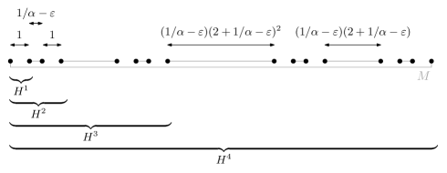
Figure 1: This extended version of the Reingold-Tarjan graph $H^{4}$ with $2^{4}$ vertices has a unique “expensive” $\alpha$-stable matching $M$. Setting the optional parameters $\alpha$ and $\varepsilon$ (that are used in the proof of the $\mathrm{PoS}$ lower bound) to $1$ and $0$, respectively, yields the original Reingold-Tarjan graph $H^{4}$.

Recall that $M^{*}(H^{k})$ matches $x_{2i-1}^{k}$ with $x_{2i}^{k}$ for every $1\leq i\leq 2^{k-1}$; since all these edges have weight $1$, it follows that $c(M^{*}(H^{k}))=2^{k-1}$. Furthermore, we argue by induction on $k$ that the matching $M(H^{k})=\{(x_{2i}^{k},x_{2i+1}^{k})\mid 1\leq i<2^{k}\}\cup\{(x_{1}^{k},x_{2^{k}}^{k})\}$ is stable; whose cost is $c(M(H^{k}))=D^{k}+(D^{k}-c(M^{*}))=2\cdot 3^{k-1}-2^{k-1}$. Therefore, $\xi_{RT}^{k}=(H^{k},M^{*}(H^{K}),M(H^{*}))$, referred to hereafter as the $k^{\text{th}}$ Reingold-Tarjan MC, is a valid weighted line MC with ratio

$$(/\xi_{RT}^{k})=\frac{c(M(H^{k}))}{c(M^{*}(H^{k}))}=\frac{2\cdot 3^{k-1}-2^{k-1}}{2^{k-1}}=\Theta\left((3/2)^{k-1}\right)=\Theta\left(n^{\log(3/2)}\right)\enspace,$$

where the last equation follows by setting $2n=2^{k}$. Combined with Lemma 3.5, we immediately conclude that $\mathrm{PoA}(2n)=\Omega(n^{\log(3/2)})$, establishing the lower bound part of Theorem 3.1. The upper bound part of the theorem is established by combining Lemmas 3.2, 3.3, 3.4, and 3.5 with the following lemma.

Lemma 3.6.

The $k^{\text{th}}$ Reingold-Tarjan MC $\xi_{RT}^{k}$ satisfies $(/\xi_{RT}^{k})\geq(/\xi)$ for any weighted line MC $\xi$ on $2^{k}$ vertices.

Proof.

By induction on $k$. The assertion holds trivially for $k=1$, so assume that it holds for $k$ and consider an arbitrary weighted line MC $\xi=(G,M^{*}(G),M(G))$ on $2^{k+1}$ vertices identified with the reals $x_{1}<\cdots<x_{2^{k+1}}$. Let $L$ and $R$ be the subgraphs of $G$ induced by the vertices $x_{1},\dots,x_{2^{k}}$ and $x_{2^{k}+1},\dots,x_{2^{k+1}}$, respectively. Let $e=(x_{2^{k}},x_{2^{k}+1})$ and let $D_{L}=x_{2^{k}}-x_{1}$ and $D_{R}=x_{2^{k+1}}-x_{2^{k}+1}$. We refer to the vertices $x_{1}$ and $x_{2^{k}}$ (respectively, $x_{2^{k}+1}$ and $x_{2^{k+1}}$) as the external vertices of $L$ (resp., $R$) and to the vertices $x_{2},\dots,x_{2^{k}-1}$ (resp., $x_{2^{k}+2},\dots,x_{2^{k+1}-1}$) as the internal vertices of $L$ (resp., $R$). Observe that $e\in M(G)$ and since $M(G)$ is a stable matching of $G$, we must have $x_{2^{k}+1}-x_{2^{k}}=w(e)\leq\min\{D_{L},D_{R}\}$ as otherwise, at least one of the edges $(x_{1},x_{2^{k}})$ or $(x_{2^{k}+1},x_{2^{k+1}})$ is unstable. Figure 2 illustrates the various notions.

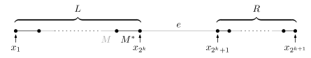
Figure 2: Any MC $\xi$ on $2^{k}$ vertices can be transformed into a Reingold-Tarjan $MC$ without decreasing the ratio $(/\xi)$. The black edges are part of the minimum-cost matching $M^{*}$ while the gray edges belong to the stable matching $M$.

We say that a $2^{k}$-vertex weighted line graph is consistent with $H^{k}$ if it can be obtained from $H^{k}$ by scaling the edge weights. Fixing the external vertices of $L$ and $R$, we argue that the internal vertices of $L$ and $R$ can be repositioned so that $L$ and $R$, respectively, become consistent with $H^{k}$ without violating the validity of $\xi$ as a weighted line MC and without decreasing the ratio $(/\xi)$. We shall establish this fact for $L$; the proof for $R$ is analogous. Note first that since $M(H^{k})$ is stable in $H^{k}$ and since $w(e)\leq D_{L}$, it follows that by repositioning the internal vertices of $L$ so that $L$ becomes consistent with $H^{K}$, we do not violate the stability of $M(G)$. Second, by the inductive hypothesis, repositioning the internal vertices of $L$ so that $L$ becomes consistent with $H^{K}$ maximizes $c(M(L))/c(M^{*}(L))$, thus $(/\xi)$ cannot decrease after this repositioning step, which establishes the argument. So, assume hereafter that both $L$ and $R$ are consistent with $H^{k}$.

Assume without loss of generality that $D_{L}\geq D_{R}$, so $w(e)=x_{2^{k}+1}-x_{2^{k}}$ is at most $D_{R}$. In fact, since $R$ is consistent with $H^{k}$, it follows that we can increase the difference $x_{2^{k}+1}-x_{2^{k}}$ until it is equal to $D_{R}$, keeping the difference $x_{i+1}-x_{i}$ unchanged for all other $i$s, without violating the validity of $\xi$ as a weighted line MC and without decreasing the ratio $(/\xi)$. So, assume hereafter that $D_{L}\geq w(e)=D_{R}$. Now, we argue that we can scale down the differences $x_{i+1}-x_{i}$ for every $1\leq i<2^{k}$, keeping $x_{i+1}-x_{i}$ unchanged for all other $i$s, until we obtain $D_{L}=w(e)=D_{R}$, without decreasing the ratio $(/\xi)$. This completes the proof since $D_{L}=w(e)=D_{R}$ implies that $G=H^{k+1}$.

Let $\ell=c(M(L))-D_{L}$, $\ell^{*}=c(M^{*}(L))$, $r=c(M(R))-D_{R}$, and $r^{*}=c(M^{*}(R))$; notice that $\ell+\ell^{*}=D_{L}$ and $r+r^{*}=D_{R}$. Since $w(e)=D_{R}$, we can express $(/\xi)$ as

$$(/\xi)=\frac{c(M(G))}{c(M^{*}(G))}=\frac{2\ell+\ell^{*}+2(r+r^{*})+2r+r^{*}}{\ell^{*}+r^{*}}=\frac{2\ell+\ell^{*}+4r+3r^{*}}{\ell^{*}+r^{*}}\enspace.$$

Recalling that $D_{L}\geq D_{R}$, we express $D_{L}$ as $D_{L}=(1+\lambda)D_{R}$ for some $\lambda\geq 0$, and so $\ell=(1+\lambda)r$ and $\ell^{*}=(1+\lambda)r^{*}$. Thus,

$$(/\xi)=\frac{2(1+\lambda)r+(1+\lambda)r^{*}+4r+3r^{*}}{(1+\lambda)r^{*}+r^{*}}=\frac{(6+2\lambda)r+(4+\lambda)r^{*}}{(2+\lambda)r^{*}}\enspace.$$

Assuming that the edge weights in $G$ (as a whole) are scaled so that $R=H^{K}$ (rather than merely being consistent with $H^{k}$), and recalling the properties of $\xi_{RT}^{k}$, we get

$$(/\xi)=\frac{(6+2\lambda)(3^{k-1}-2^{k-1})+(4+\lambda)2^{k-1}}{(2+\lambda)2^{k-1}}=\left(\frac{6+2\lambda}{2+\lambda}\right)\cdot(3/2)^{k-1}-1\enspace.$$

The lemma follows since the function $f(\lambda)=\frac{6+2\lambda}{2+\lambda}$ is monotonically decreasing for $\lambda\geq 0$. ∎

4 $\alpha$-Price of Stability

The upper bound established in Sect. 3 for the $\mathrm{PoA}$ clearly holds for the $\mathrm{PoS}$ too; the matching lower bound can be adapted to the $\mathrm{PoS}$ by slightly modifying the Reingold-Tarjan graphs so that they admit a unique stable matching (see Sect. 4.4), implying that $\mathrm{PoS}(2n)=\Theta(n^{\log(3/2)})$. So, the $\mathrm{PoS}$ does not provide much of an improvement over the $\mathrm{PoA}$. Consequently, we turn to analyze the $\mathrm{PoS}$ with respect to relaxed stable matchings, establishing the following theorem.

Theorem 4.1.

The $\alpha$-$\mathrm{PoS}$ of minimum-cost perfect matchings in metric graphs with $2n$ vertices is $\Theta(n^{\log(1+1/(2\alpha))})$. In particular, taking $\alpha=\mathcal{O}(\log n)$ guarantees a constant $\mathrm{PoS}$.

The upper bound promised by Theorem 4.1 is constructive, relying on an efficient greedy algorithm presented in Sect. 4.1. Sect. 4.2 provides a simplified version of the analysis of that greedy algorithm that holds only for the case of $\alpha=\mathcal{O}(\log n)$. A more involved analysis that covers the general case is given in Sect. 4.3. The matching $\Omega(n^{\log(1+1/(2\alpha))})$ lower bound on $\mathrm{PoS}_{\alpha}(2n)$ is established via a generalization of the Reingold-Tarjan graphs in Sect. 4.4.

4.1 Greedy Algorithm for $\alpha$-Stable Matchings

The following algorithm called Greedy transforms a minimum-cost matching $M^{*}$ in a metric graph into an $\alpha$-stable matching $M$.

Start with the minimum-cost matching $M\leftarrow M^{*}$ and iterate over all edges of $G$ by non-decreasing order of weights. If the edge $(u,v)$ currently considered is unstable with respect to the current matching $M$, set $M\leftarrow M\cup\{(u,v),\ (M(u),M(v))\}-\{(u,M(u)),\ (v,M(v))\}$ (this operation is called a flip of the edge $(u,v)$) and continue with the next edge. After having iterated over all edges, return $M$.

We assume that edge weight ties are resolved in an arbitrary but consistent manner. In the following, we denote by $M_{i}$ the matching calculated by the above algorithm at the end of iteration $i$. Moreover, $M_{0}=M^{*}$ is the initial minimum-cost matching and $M_{G}$ the final matching returned by Greedy. The following lemma shows that the algorithm terminates.

Lemma 4.2.

For any unstable edge $b$ created by the flip of an edge $e$, we have $w(b)>w(e)$.

Proof.

We consider the edge $e=(u,v)$ being flipped and we denote by $e^{\prime}=(M(u),M(v))$ the second new edge joining $M$ as a result of the flip. The two edges that are removed by the flip are denoted by $f$ and $g$. See Fig. 3 for an illustration of the situation.

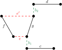
Figure 3: This figure illustrates the two different cases of Lemma 4.2.

When an edge $e$ is flipped, there are essentially two different cases for an unstable edge to be created. Either the unstable edge contains one vertex of $e$ or one vertex of $e^{\prime}$. No other vertices are involved in the flip and thus every new unstable edge has to contain at least one of the four vertices. We assume without loss of generality that a vertex of the edge $g$ is incident to the unstable edge created by the flip.

Let us first consider the case where a vertex of $e$ is incident to the new unstable edge. This case is denoted as the edge $b_{1}$ in Fig. 3. We assume that $b_{1}$ is stable before the flip and unstable thereafter. For $b_{1}$ to be unstable after the flip, we must have $\alpha\cdot w(b_{1})<w(e)$ and $\alpha\cdot w(b_{1})<w(c)$. But as $e$ is unstable before the flip, we have $\alpha\cdot w(e)<w(g)$ and thus we get $\alpha\cdot w(b_{1})<w(e)<w(g)/\alpha\leq w(g)$. This means that $b_{1}$ was already unstable before the flip, which is a contradiction to the assumption. Hence, no vertex of $e$ can be part of the new unstable edge.

Let us now consider the case, where a vertex from $e^{\prime}$ is part of the new unstable edge ($b_{2}$ in Fig. 3). Since $b_{2}$ is stable before the flip and unstable after it, we must have $w(g)\leq\alpha\cdot w(b_{2})<w(e^{\prime})$. But as $e$ is unstable before the flip, we have $\alpha\cdot w(e)<w(g)$, and thus we get $w(e)<w(g)/\alpha\leq w(b_{2})$ which completes the proof. ∎

Corollary 4.3 follows by induction on $i$.

Corollary 4.3.

Let $e_{i}$ be the edge considered in iteration $i$. Then $w(e_{i})<w(b)$ for any unstable edge $b$ in $M_{i}$.

Lemma 4.4.

Greedy transforms a minimum-cost matching into a valid $\alpha$-stable matching in time $\mathcal{O}(n^{2}\log n)$.

Proof.

The running time of the algorithm is dominated by the step of sorting the edges in $G$ according to their weight. This takes $\mathcal{O}(n^{2}\log n)$ steps. The second phase — the actual algorithm — runs in $\mathcal{O}(n^{2})$ steps since it iterates once over all edges in $V\times V$ and each iteration takes $\mathcal{O}(1)$ time.

The correctness of the algorithm is established by Corollary 4.3 since it states that in the last iteration, all unstable edges have strictly larger weight than the edge currently considered. Since this edge is already the one with the largest weight, there cannot be any unstable edges in the final matching $M_{G}$. ∎

4.2 Cost Analysis

In this section, we want to bound the cost of the $\alpha$-stable matching returned by Greedy relative to the cost of $M^{*}$. To this end, we will transcribe the changes that Greedy performs on the minimum-cost matching through a collection of logical rooted trees, referred to as the flip forest, and assign weights to the nodes of the trees in this forest that will then allow us to derive an upper bound on the cost of the $\alpha$-stable matching returned by the algorithm.

Since this section makes heavy use of rooted binary trees and their properties, we require a few definitions. In a full binary tree, each inner node has exactly two children. The depth $d(v)$ of a node $v$ in a tree $T$ is the length of the unique path from the root of $T$ to $v$ and the height $h(T)$ of a tree $T$ is defined as the maximal depth of any node in $T$. The height $h(v)$ of a node $v$ of $T$ is defined to be the height of its subtree. The leaf set $\mathcal{L}(T)$ or $\mathcal{L}(F)$ of a tree $T$ or a collection $F$ of trees is the set of all leaves in $T$ or $F$, respectively. The leaf set $\mathcal{L}(v)$ of a node $v$ in a tree is $\mathcal{L}(T_{v})$ where $T_{v}$ is the subtree rooted at $v$. Finally, two nodes with the same parent are called sibling nodes.

We begin with Lemma 4.5 stating an important property of the edges that are flipped by Greedy.

Lemma 4.5.

If an edge $e$ is flipped in iteration $i$, then $e\in M_{j}$ for all $j\geq i$ and in particular $e\in M_{G}$.

Proof.

Let us assume for the sake of contradiction that $e=(u,v)$ was flipped in iteration $i$ of the algorithm and further that $(u,v)\notin M_{j}$ for some $j>i$. According to the algorithm, we have $(u,v)\in M_{i}$. Since $(u,v)\notin M_{j}$, there has to exist an iteration $k$ with $i<k\leq j$ where $(u,v)$ is removed from $M_{k-1}$ such that $(u,v)\notin M_{k}$. For this to happen, either edge $(u,u^{\prime})$ or $(v,v^{\prime})$ for some vertex $u^{\prime}$ or $v^{\prime}$ must be flipped in iteration $k$ because it was unstable with respect to $M_{k-1}$. Without loss of generality, we assume that $(u,u^{\prime})$ is unstable with respect to $M_{k-1}$ and flipped in iteration $k>i$ and we have

$$\ignorespaces w(u,u^{\prime})~{}\leq~{}\alpha\cdot w(u,u^{\prime})<w(u,v)\enspace.$$

But this means that Greedy would have considered the edge $(u,u^{\prime})$ before considering the edge $(u,v)$, a contradiction to the assumption. ∎

Consider an iteration of Greedy where edge $(u,v)$ is flipped because it was unstable at the beginning of the iteration. Then the two edges $(u,M(u))$ and $(v,M(v))$ are replaced by $(u,v)$ and $(M(u),M(v))$. Since, according to Lemma 4.5, the edge $(u,v)$ is selected irrevocably, the edges $(u,M(u))$ and $(v,M(v))$ can never be part of $M$ again. The only edge, of the four edges involved, that may be changed again, is the edge $(M(u),M(v))$. Thus, we refer to $(M(u),M(v))$ as an active edge. We also refer to all edges in $M_{0}$ as active. Using the notion of active edges, we shall now model the changes that Greedy applies to the matching during its execution through a logical helper structure called the flip forest.

Definition (Flip Forest).

The flip forest $F=(U,K)$ for a certain execution of Greedy is a collection of rooted trees with node set $U$ and link set $K$. It contains a node $u_{e}\in U$ corresponding to each edge $e\in V\times V$ that has been active at some stage during the execution. This correspondence is denoted by $u_{e}\sim e$. For each flip of an edge $(u,v)$ in $G$, resulting in the removal of the edges $(u,M(u))$ and $(v,M(v))$ from $M$, $K$ contains a link connecting the node $y\sim(u,M(u))$ to its parent $x\sim(M(u),M(v))$ and a link connecting the node $z\sim(v,M(v))$ to its parent $x\sim(M(u),M(v))$. (Observe that by definition, all three edges $(u,M(u))$, $(v,M(v))$, and $(M(u),M(v))$ are active.) Refer to Fig. 4 for an illustration.

Figure 4: The left side shows a matching configuration with an unstable edge $(u,v)$, which will be flipped by Greedy. This flip is then represented by the flip tree segment on the right, which depicts the replacement of the two active edges $(u,M(u))\sim y$ and $(v,M(v))\sim z$ by the active edge $(M(u),M(v))\sim x$.

To avoid confusion between the basic elements of $G$ and the basic elements of $F$, we refer to the former as vertices/edges and to the latter as nodes/links.

The definition of a flip forest ensures that for each flip of the algorithm, we obtain a binary flip tree segment as depicted by Fig. 4. When we transcribe each flip operation of the complete execution of Greedy into a flip tree segment as explained above, we end up with a collection of full binary trees — a forest as depicted in Fig. 5. This is because the parent node of a tree segment may appear as a child node of the tree segment corresponding to a later iteration of the algorithm since its corresponding edge is still active and therefore may participate in another flip. Each such tree is called a flip tree hereafter. Observe that all leaves in the flip forest correspond to edges in the minimum-cost matching $M_{0}=M^{*}$.

Figure 5: All leaves and isolated nodes of the flip forest $F$ correspond to edges in the minimal-cost matching $M^{*}$. Each inner node corresponds to the active edge that resulted from the respective flip. Note that the edge that got flipped and is therefore irrevocably selected into $M_{G}$ has no corresponding node in $F$. For the purpose of illustration, we can associate such an edge with the respective node as indicated by a line below the respective inner node. These edges constitute the matching $M_{G}$ together with the edges corresponding to isolated vertices and roots, indicated by a line above the node.

We now define a function $\psi:U\mapsto\mathbb{R}$ that maps a virtual weight to each node in the flip forest $F$ as follows. For each leaf $\ell$ of a flip tree in $F$, we set $\psi(\ell)\coloneqq w(e)$, where $\ell\sim e$ and we recall that an edge corresponding to a leaf node in $F$ is part of $M^{*}$. The function $\psi$ is extended to an inner node $x$ of a flip tree with child nodes $y$ and $z$ by the recursion

$$\psi(x)\coloneqq\psi(y)+\psi(z)+(1/\alpha)\cdot\min\{\psi(y),\psi(z)\}\enspace.$$ (1)

For the ease of argumentation, we call the child with smaller (respectively, larger) value of $\psi$ as well as the link leading to its parent light (resp., heavy). We denote the light child of a node $x$ as ${x}_{{}_{\!L\!}}$ and the heavy child as ${x}_{{}_{\!H\!}}$. Then we can rewrite the recursion from Eq. 1 as

$$\ignorespaces\psi(x)\coloneqq\psi({x}_{{}_{\!H\!}})+(1+1/\alpha)\cdot\psi({x}_{{}_{\!L\!}})\enspace.$$

Lemma 4.6.

Let $x$ be a node in $F$ and $e$ an edge in $G$ with $x\sim e$. Then $w(e)\leq\psi(x)$.

Proof.

We prove the statement by induction over the height of $x$ in its flip tree. The assertion holds for every leaf $x\sim e$ in the flip forest as $\psi(x)=w(e)$ by definition. Assume that the statement holds for the two children ${x}_{{}_{\!L\!}}$ and ${x}_{{}_{\!H\!}}$ of a node $x$ that represents a flip of the edge $(u,v)$. Then $x\sim(M(u),M(v))=e$ and we assume without loss of generality that ${x}_{{}_{\!H\!}}\sim(u,M(u))=e_{u}$ and ${x}_{{}_{\!L\!}}\sim(v,M(v))=e_{v}$. Thus, $w(e_{u})\leq\psi({x}_{{}_{\!H\!}})$ and $w(e_{v})\leq\psi({x}_{{}_{\!L\!}})$. This flip tree segment represents the replacement of the edges $e_{u}$ and $e_{v}$ by $e$ and $(u,v)$, which happened because the edge $(u,v)$ was unstable with respect to $M$, that is, $\alpha\cdot w(u,v)<\min\{w(e_{v}),w(e_{u})\}$. Since $G$ is metric, we can bound $w(e)$ as

$$w(e)~{} \leq~{}w(e_{u})+w(e_{v})+w(u,v)$$

$$<~{}w(e_{u})+(1+1/\alpha)\cdot w(e_{v})$$

$$\leq~{}\psi({x}_{{}_{\!H\!}})+(1+1/\alpha)\cdot\psi({x}_{{}_{\!L\!}})$$ (inductive hypothesis)

$$=~{}\psi(x)\enspace.$$ ∎

Definition (Light Depth).

The light depth $\lambda(x)$ of a node $x$ in a flip forest $F$ is the number of light links on the direct path from $x$ to the root of the flip tree containing $x$.

Lemma 4.7.

Every node $x$ in a flip tree satisfies

$$\ignorespaces\psi(x)~{}=~{}\sum_{\ell\in\mathcal{L}(x)}(1+1/\alpha)^{\lambda(\ell)-\lambda(x)}\cdot\psi(\ell)\enspace.$$

Proof.

We prove the statement by induction over the height of $x$ in its flip tree. The statement holds for a leaf node $x$ since then we have $\mathcal{L}(x)=\{x\}$ and $\lambda(x)-\lambda(x)=0$. Assume that the statement holds for both children ${x}_{{}_{\!H\!}}$ and ${x}_{{}_{\!L\!}}$ of a node $x$. By definition, we have

$$\psi(x)~{} =~{}\psi({x}_{{}_{\!H\!}})+(1+1/\alpha)\cdot\psi({x}_{{}_{\!L\!}})$$

$$=~{}\sum_{\ell\in\mathcal{L}({x}_{{}_{\!H\!}})}(1+1/\alpha)^{\lambda(\ell)-\lambda({x}_{{}_{\!H\!}})}\cdot\psi(\ell)+(1+1/\alpha)\cdot\sum_{\ell\in\mathcal{L}({x}_{{}_{\!L\!}})}(1+1/\alpha)^{\lambda(\ell)-\lambda({x}_{{}_{\!L\!}})}\cdot\psi(\ell)$$

$$=~{}\sum_{\ell\in\mathcal{L}({x}_{{}_{\!H\!}})}(1+1/\alpha)^{\lambda(\ell)-\lambda(x)}\cdot\psi(\ell)+(1+1/\alpha)\cdot\sum_{\ell\in\mathcal{L}({x}_{{}_{\!L\!}})}(1+1/\alpha)^{\lambda(\ell)-\lambda(x)-1}\cdot\psi(\ell)$$

$$=~{}\sum_{\ell\in\mathcal{L}({x}_{{}_{\!H\!}})}(1+1/\alpha)^{\lambda(\ell)-\lambda(x)}\cdot\psi(\ell)+\sum_{\ell\in\mathcal{L}({x}_{{}_{\!L\!}})}(1+1/\alpha)^{\lambda(\ell)-\lambda(x)}\cdot\psi(\ell)$$

$$=~{}\sum_{\ell\in\mathcal{L}(x)}(1+1/\alpha)^{\lambda(\ell)-\lambda(x)}\cdot\psi(\ell)\enspace,$$

where we used $\lambda({x}_{{}_{\!L\!}})=\lambda(x)+1$ and $\lambda({x}_{{}_{\!H\!}})=\lambda(x)$. ∎

Corollary 4.8 is immediate, since $\lambda(r_{T})=0$ for the root $r_{T}$ of a flip tree $T$.

Corollary 4.8.

The root $r_{T}$ of a flip tree $T$ satisfies

$$\ignorespaces\psi(r_{T})~{}=~{}\sum_{\ell\in\mathcal{L}(r_{T})}(1+1/\alpha)^{\lambda(\ell)}\cdot\psi(\ell)\enspace.$$

The following observation stems from the fact that in each segment, the $\psi$-value of the parent is at least $(2+1/\alpha)$ times that of the light child (equality holds when both children have the same $\psi$-value).

Observation 4.9.

For any flip tree $T$ with root $r_{T}$ and any leaf $\ell$ of $T$, we have

$$\ignorespaces\psi(r_{T})~{}\geq~{}(2+1/\alpha)^{\lambda(\ell)}\cdot\psi(\ell)\enspace.$$

We now turn to bound $\psi(r_{T})$ for all trees $T\in F$ with respect to the sum of the weights of the edges that correspond to the leaves of $T$. Since all these edges are part of $M^{*}$ by construction of $F$, this will allow us to bound the cost of $M_{G}$ with respect to $M^{*}$.

Lemma 4.10.

The virtual weights in a flip tree $T$ satisfy

$$\ignorespaces\psi(r_{T})~{}=~{}\mathcal{O}\Big{(}(1+1/\alpha)^{\log n}\sum_{\ell\in\mathcal{L}(r_{T})}\psi(\ell)\Big{)}\enspace.$$

Proof.

Corollary 4.8 implies that $\psi(r_{T})=\sum_{\ell\in\mathcal{L}(r_{T})}(1+1/\alpha)^{\lambda(\ell)}\cdot\psi(\ell)$. We group the leaves according to their light depth, where $\mathcal{L}_{j}$ denotes the set of leaves $\ell$ of $T$ with $\lambda(\ell)=j$. The equation for $\psi(r_{T})$ can now be rewritten as $\psi(r_{T})=\sum_{j=0}^{n}\ \sum_{\ell\in\mathcal{L}_{j}}(1+1/\alpha)^{j}\cdot\psi(\ell)$. Let $\Psi^{>}=\sum_{j=j^{\prime}}^{n}\sum_{\ell\in\mathcal{L}_{j}}(1+1/\alpha)^{j}\cdot\psi(\ell)$ for some $j^{\prime}$ that will soon be determined. We apply Observation 4.9 and the fact that there are at most $n$ leaves in $T$ altogether to conclude

$$\Psi^{>}~{} =~{}\sum_{j=j^{\prime}}^{n}\ \sum_{\ell\in\mathcal{L}_{j}}(1+1/\alpha)^{j}\cdot\psi(\ell)$$

$$\leq~{}\sum_{j=j^{\prime}}^{n}\ \sum_{\ell\in\mathcal{L}_{j}}\left(\frac{1+1/\alpha}{2+1/\alpha}\right)^{\!\!j}\cdot\psi(r_{T})$$

$$=~{}\sum_{j=j^{\prime}}^{n}|\mathcal{L}_{j}|\left(\frac{1+1/\alpha}{2+1/\alpha}\right)^{\!\!j}\cdot\psi(r_{T})$$

$$\leq~{}n\cdot\left(\frac{1+1/\alpha}{2+1/\alpha}\right)^{\!\!j^{\prime}}\cdot\psi(r_{T})\enspace.$$

Choosing $j^{\prime}=\log_{\frac{2+1/\alpha}{1+1/\alpha}}(2n)=\mathcal{O}(\log n)$ yields $\Psi^{>}\leq\psi(r_{T})/2$. This means that the leaves with light depth at most $c\log n$ for some constant $c$ contribute at least half of $\psi(r_{T})$ and thus it suffices to consider only those leaves in order to bound $\psi(r_{T})$:

$$\psi(r_{T}) ~{}\leq~{}2\cdot\sum_{j=0}^{c\log n}\ \sum_{\ell\in\mathcal{L}_{j}}(1+1/\alpha)^{j}\cdot\psi(\ell)~{}\leq~{}2\cdot(1+1/\alpha)^{c\log n}\sum_{\ell\in\mathcal{L}(r_{T})}\psi(\ell)\enspace.$$ ∎

At this stage, we would like to relate the virtual weight $\psi(r_{T})$ of the roots $r_{T}$ in $F$ to the cost of the stable matching $M_{G}$ returned by Greedy. To that end, we observe that $M_{G}$ consists of the edges corresponding to the roots in $F$ and to the edges that have been flipped along the course of the execution; let $D$ denote the set of the latter edges.

Consider the flip of edge $(u,v)$, resulting in the insertion of edge $(M(u),M(v))\sim x$ to $M$ and the removal of edges $(u,M(u))\sim x_{L}$ and $(v,M(v))\sim x_{H}$ from $M$. Since $\psi(x)=\psi(x_{H})+(1+1/\alpha)\psi(x_{L})$, we have $\psi(x)-(\psi(x_{L})+\psi(x_{H}))=\psi(x_{L})/\alpha$. Lemma 4.6 then implies that $\psi(x)-(\psi(x_{L})+\psi(x_{H}))\geq w(u,M(u))/\alpha$, and since edge $(u,v)$ was flipped, we have $\psi(x)-(\psi(x_{L})+\psi(x_{H}))\geq w(u,v)$. Therefore,

$$\sum_{e\in D}w(e)~{}\leq~{}\sum_{\text{internal }x\in U}\left(\psi(x)-(\psi(x_{L})+\psi(x_{H}))\right)~{}=~{}\sum_{\text{flip trees T}}\Big{(}\psi(r_{T})-\sum_{\ell\in\mathcal{L}(T)}\psi(\ell)\Big{)}\enspace,$$

where the second equation holds by a telescoping argument. Corollary 4.11 follows since $c(M^{*})=\sum_{\ell\in\mathcal{L}(F)}\psi(\ell)$.

Corollary 4.11.

The matching $M_{G}$ returned by Greedy satisfies $c(M_{G})\leq 2\sum_{\text{\rm flip trees $T$}}\psi(r_{T})-c(M^{*})$.

We are now ready to establish the following lemma.

Lemma 4.12.

The cost of the matching $M_{G}$ returned by Greedy for $\alpha=\mathcal{O}(\log n)$ is an $\mathcal{O}(1)$ approximation of $c(M^{*})$.

Proof.

Employing Lemma 4.10 and setting $\alpha=\mathcal{O}(\log n)$, we get $\psi(r_{T})=\mathcal{O}\big{(}\!\sum_{\ell\in\mathcal{L}(T)}\psi(\ell)\big{)}$. Corollary 4.11 and the fact that $c(M^{*})=\sum_{\ell\in\mathcal{L}(F)}\psi(\ell)$ then imply that $c(M_{G})=\mathcal{O}(c(M^{*}))$ as desired. ∎

4.3 Tight Upper Bound

Our goal in this section is to show that when Greedy is invoked with parameter $\alpha$ for any $\alpha\geq 1$, it returns an $\alpha$-stable matching $M_{G}$ satisfying $c(M_{G})=c(M^{*})\cdot\mathcal{O}(n^{\log(1+1/(2\alpha))})$. This is performed by taking a deeper examination of the properties of our flip trees and their virtual weights. It will be convenient to ignore the relation of the flip trees to the Greedy algorithm at this stage; in other words, we consider an abstract full binary tree $T$ with a function $w:\mathcal{L}(T)\rightarrow\mathbb{R}_{\geq 0}$ that assigns non-negative weights to the leaves of $T$, which then determines the virtual weight $\psi(x)$ of each node in $T$, following the recursion of Eq. (1). Note that we allow our tree $T$ to have zero-weight leaves now (this can only make our analysis more general).

Definition (Complete Binary Tree).

A full binary tree $T$ is called complete if all leaves are at depth $h(T)$ or $h(T)-1$. Given some positive integer $n$ that will typically be the number of leaves in some tree, let

$$h(n)=\lceil\log n\rceil\quad\text{ and }\quad k(n)=2^{h(n)}-n\enspace.$$

Note that $0\leq k(n)<2^{h(n)-1}$.

Definition ($\psi$-Balanced Flip Tree).

A full binary tree $T$ is called $\psi$-balanced if for any two sibling nodes $x,y$ in $T$, we have $\psi(x)=\psi(y)$.

Consider some full binary tree $T$. Let $\Lambda(T)$ denote the sum of the virtual weights of $T$’s leaves, that is, $\Lambda(T)=\sum_{\ell\in\mathcal{L}(T)}\psi(\ell)$, and let $\Psi(T)=\psi(r_{T})$ (recall that $r_{T}$ denotes the root of $T$). The following observation is established by induction on the depth of the nodes.

Observation 4.13.

For any node $v$ of a $\psi$-balanced full binary tree $T$, we have $\psi(v)=(2+1/\alpha)^{-d(v)}\cdot\Psi(T)$.

Definition (Effect of a Flip Tree).

The effect $\eta(T)$ of a full binary tree $T$ is defined to be

$$\eta(T)~{}=~{}\begin{cases}\Psi(T)/\Lambda(T)&\text{if }\Lambda(T)>0\\ 1&\text{if }\Lambda(T)=0\end{cases}\enspace.$$

An $n$-leaf full binary tree $T$ is said to be effective if it maximizes $\eta(T)$, namely, if there does not exist any $n$-leaf full binary tree $T^{\prime}$ such that $\eta(T^{\prime})>\eta(T)$.

Intuitively speaking, if we think of $T$ as a flip tree, then its effect is a measure for the factor by which the flips represented by $T$ increase the cost of $M^{*}$ when applied to it. But, once again, we do not restrict our attention to flip trees at this stage. The effect of a full binary tree is essentially determined by its topology and by the assignment of weights to its leaves. It is important to point out that by Corollary 4.8, the effect of a full binary tree is not affected by scaling its leaf weights. Our upper bound is established by showing that the effect of an effective $n$-leaf full binary tree is $\mathcal{O}\left(n^{\log(1+1/(2\alpha))}\right)$. We begin by developing a better understanding of the topology of effective $\psi$-balanced full binary trees.

Lemma 4.14.

An effective $n$-leaf $\psi$-balanced full binary tree must be complete.

Proof.

Aiming for a contradiction, suppose that $T$ is not complete and scale the leaf weights in $T$ so that $\Psi(T)=1$. Because $T$ is not complete, it must have leaves at depth $d_{1}$ and at depth $d_{2}$, where $d_{2}>d_{1}+1$. The assertion is established by showing that an $n$-leaf full binary tree with higher effect can be obtained by a small modification to $T$’s topology, in contradiction to the assumption that $T$ is effective.

Let $y$ be a leaf at depth $d_{1}$ and $\ell_{1}$ and $\ell_{2}$ be two leaves at depth $d_{2}>d_{1}+1$ with parent node $z$. Since $T$ is $\psi$-balanced, we can employ Observation 4.13 to conclude that $\psi(\ell_{1})=\psi(\ell_{2})=(2+1/\alpha)^{-d_{2}}$ and $\psi(y)=(2+1/\alpha)^{-d_{1}}$.

Now, consider the $\psi$-balanced full binary tree $T^{\prime}$ obtained from $T$ by removing $\ell_{1}$ and $\ell_{2}$ and adding two new leaves $\ell^{\prime}_{1}$ and $\ell^{\prime}_{2}$ as children of $y$ with virtual weight $\psi(\ell^{\prime}_{1})=\psi(\ell^{\prime}_{2})=(2+1/\alpha)^{-d_{1}-1}$, keeping the virtual weight of all other nodes unchanged. By doing so, we turn $z$ — an internal node in $T$ — into a leaf (whose virtual weight remains $\psi(z)=(2+1/\alpha)^{-d_{2}+1}$). On the other hand, $y$ which is a leaf in $T$, is an internal node in $T^{\prime}$. Therefore,

$$\Lambda(T^{\prime})~{}=~{} \Lambda(T)+\psi(\ell^{\prime}_{1})+\psi(\ell^{\prime}_{2})+\psi(z)-\psi(\ell_{1})-\psi(\ell_{2})-\psi(y)$$

$$=~{} \Lambda(T)+2\cdot(2+1/\alpha)^{-d_{1}-1}+(2+1/\alpha)^{-d_{2}+1}-2\cdot(2+1/\alpha)^{-d_{2}}-(2+1/\alpha)^{-d_{1}}$$

$$=~{} \Lambda(T)+(2+1/\alpha)^{-d_{1}-1}(2-(2+1/\alpha))+(2+1/\alpha)^{-d_{2}}(2+1/\alpha-2)$$

$$=~{} \Lambda(T)+(1/\alpha)((2+1/\alpha)^{-d_{2}}-(2+1/\alpha)^{-d_{1}-1})$$

$$<~{} \Lambda(T)\enspace.$$

As $\Psi(T^{\prime})=\Psi(T)=1$, it follows that $\eta(T^{\prime})>\eta(T)$, in contradiction to the effectiveness of $T$. ∎

Next, we develop a closed-form expression for the effect of complete $\psi$-balanced full binary trees.

Lemma 4.15.

The effect of an $n$-leaf complete $\psi$-balanced full binary tree $T$ is

$$\eta(T)=\frac{(2+1/\alpha)^{h}}{2^{h}+k/\alpha}\enspace,$$

where $h=h(n)$ and $k=k(n)$.

Proof.

Again we assume without loss of generality that the weights of the leaves are scaled so that $\Psi(T)=1$. By definition, $T$ has $2^{h}-2k$ leaves at depth $h$ and $k$ leaves at depth $h-1$. Employing Observation 4.13, we conclude

$$\Lambda(T)~{}=~{} (2^{h}-2k)\cdot(2+1/\alpha)^{-h}+k\cdot(2+1/\alpha)^{-(h-1)}$$

$$=~{} (2+1/\alpha)^{-h}\cdot(2^{h}-2k+k\cdot(2+1/\alpha))$$

$$=~{} (2+1/\alpha)^{-h}\cdot(2^{h}+k/\alpha)\enspace.$$

Since $\Psi(T)=1$, we have $\eta(T)=1/\Lambda(T)$ which completes the proof. ∎

Note that the expression for the effect of an $n$-leaf complete $\psi$-balanced full binary tree given by Lemma 4.15 is monotonically increasing with $h$ and monotonically decreasing with $k$. We are now ready to show that it is essentially sufficient to consider complete $\psi$-balanced full binary trees.

Lemma 4.16.

An effective $n$-leaf full binary tree must be $\psi$-balanced.

Proof.

We prove the statement by induction on the number of leaves $n$. The base case of a tree having a single leaf (which is also the root) holds vacuously; the base case of a tree having two leaves is trivial. Assume that the assertion holds for trees with less than $n$ leaves and let $T$ be an effective $n$-leaf full binary tree. Let $T_{L}$ and $T_{H}$ be the subtrees rooted at the light and heavy, respectively, children of $r_{T}$ (break ties arbitrarily). Let $n_{L}$ and $n_{H}$ be the number of leaves in $T_{L}$ and $T_{H}$, respectively, where $n_{L}+n_{H}=n$ and $0<n_{L},n_{H}<n$. Observe that since $\eta(T)=\frac{\Psi(T_{H})+(1+1/\alpha)\cdot\Psi(T_{L})}{\Lambda(T_{H})+\Lambda(T_{L})}$, both $T_{L}$ and $T_{H}$ have to be effective as otherwise, $\eta(T)$ could be increased; more precisely, if $T_{i}\in\{T_{H},\,T_{L}\}$ is not effective, then one can increase $\Psi(T_{i})$ while keeping $\Lambda(T_{i})$ unchanged, which results in an increased $\eta(T)$. Thus, by the inductive hypothesis, we conclude that $T_{L}$ and $T_{H}$ must be $\psi$-balanced. Lemma 4.14 then guarantees that both $T_{L}$ and $T_{H}$ are complete.

Aiming for a contradiction, suppose that $T$ is not $\psi$-balanced, that is $\Psi(T_{H})>\Psi(T_{L})$. Assume without loss of generality that the leaf weights are scaled such that $\Lambda(T)=\Lambda(T_{H})+\Lambda(T_{L})=1$ and set $\Lambda(T_{L})=x$, $\Lambda(T_{H})=1-x$, for some $0\leq x\leq 1$. Let $T$ be the tree minimizing $x$ among all trees satisfying the aforementioned assumptions.

We argue that $x$ cannot be neither $0$ nor $1$. Indeed, if $x=1$, then $\Psi(T_{H})=0$, in contradiction to the assumption that $\Psi(T_{H})>\Psi(T_{L})$. On the other hand, if $x=0$, then $\Psi(T)=\Psi(T_{H})$ and $\Lambda(T)=\Lambda(T_{H})$, hence $\eta(T)=\eta(T_{H})$. But since $T_{H}$ has $n_{H}<n$ leaves, Lemma 4.15 guarantees that its effect is smaller than that of an $n$-leaf complete $\psi$-balanced full binary tree, in contradiction to the assumption that $T$ is effective.

So, we may subsequently assume that $0<x<1$. Employing Lemma 4.15, we can express $\Psi(T)$ as

$$\Psi(T)~{}=~{}\Psi(T_{H})+(1+1/\alpha)\cdot\Psi(T_{L})~{}=~{}\frac{(2+1/\alpha)^{h_{H}}}{2^{h_{H}}+k_{H}/\alpha}\cdot(1-x)+(1+1/\alpha)\cdot\frac{(2+1/\alpha)^{h_{L}}}{2^{h_{L}}+k_{L}/\alpha}\cdot x\enspace,$$

where $h_{H}=h(n_{H})$, $k_{H}=k(n_{H})$, $h_{L}=h(n_{L})$, and $k_{L}=k(n_{L})$. Using this expression, we can formulate $\eta(T)$ as a function $f=f(x)$, setting

$$f(x)~{}=~{}\frac{(2+1/\alpha)^{h_{H}}}{2^{h_{H}}+k_{H}/\alpha}\cdot(1-x)+(1+1/\alpha)\cdot\frac{(2+1/\alpha)^{h_{L}}}{2^{h_{L}}+k_{L}/\alpha}\cdot x\enspace.$$ (2)

The crucial observation now is that $f(x)$ is linear in $x$, thus $\frac{\mathrm{d}f}{\mathrm{d}x}(x)$ is independent of $x$. Moreover, since $T$ is not $\psi$-balanced, it follows that $f$ is well defined — that is, Eq. (2) remains valid — in a neighborhood of $x=\Lambda(T_{L})$. Therefore, if, $\frac{\mathrm{d}f}{\mathrm{d}x}(x)>0$, then $f(x)=\eta(T)$ can be increased by increasing $x$ (shifting weight from the leaves of $T_{H}$ to the leaves of $T_{L}$), in contradiction to the effectiveness of $T$. On the other hand, if $\frac{\mathrm{d}f}{\mathrm{d}x}(x)\leq 0$, then we can decrease $x$ (shifting weight from the leaves of $T_{L}$ to the leaves of $T_{H}$) without decreasing $f(x)=\eta(T)$, contradicting the assumption that $x$ is minimum. The assertion follows. ∎

Recalling that $h=h(n)$ and $k=k(n)$, we observe that

$$\frac{(2+1/\alpha)^{h}}{2^{h}+k/\alpha}~{}=~{}\Theta\!\left((1+1/(2\alpha))^{h}\right)~{}=~{}\Theta\!\left(n^{\log(1+1/(2\alpha))}\right)\enspace.$$

Combined with Lemmas 4.14, 4.15, and 4.16, we get the following corollary.

Corollary 4.17.

The effect of an $n$-leaf full binary tree is $\mathcal{O}\!\left(n^{\log(1+1/(2\alpha))}\right)$.

Now, let us return the focus to our flip forest. Recalling that $\sum_{\text{flip trees }T}\sum_{\ell\in\mathcal{L}(T)}\psi(\ell)=c(M^{*})$, and using Corollary 4.11, we conclude that

$$\frac{c(M_{G})}{c(M^{*})}~{}=~{}\mathcal{O}\!\left(\frac{\sum_{\text{flip trees }T}\Psi(T)}{\sum_{\text{flip trees }T}\Lambda(T)}\right)~{}=~{}\mathcal{O}\!\left(\max_{\text{flip trees }T}\frac{\Psi(T)}{\Lambda(T)}\right)~{}=~{}\mathcal{O}\!\left(\max_{\text{flip trees }T}\eta(T)\right)\enspace.$$

The desired upper bound then follows from Corollary 4.17.

4.4 Lower Bound

Our goal in this section is to establish the lower bound of Theorem 4.1. The graph construction that lies at the heart of this lower bound, denoted $H^{k}_{\alpha}$, is a direct generalization of the Reingold-Tarjan graph $H^{k}$ presented in Sect. 3 for arbitrary values of $\alpha$. Specifically, the $2$-vertex graph $H^{1}_{\alpha}$ is identical to $H^{1}$; and the $2^{k+1}$-vertex graph $H^{k+1}_{\alpha}$ is constructed recursively by placing $2$ disjoint instances of $H^{k}_{\alpha}$, each of diameter $D^{k}_{\alpha}$, on the real line, only that this time, the spacing between them is set to $S^{k+1}_{\alpha}=(1/\alpha-\varepsilon)D^{k}_{\alpha}$, for some sufficiently small $\varepsilon>0$ that will be determined later on. This implies that $D^{k}_{\alpha}=(2+1/\alpha-\varepsilon)^{k-1}$ and $S^{k+1}_{\alpha}=(1/\alpha-\varepsilon)(2+1/\alpha-\varepsilon)^{k-1}$.

Now let $M$ be an $\alpha$-stable matching in $H^{k}_{\alpha}$. We argue that $M$ has to contain each edge $e=(x,y)$ with $w(e)=1/\alpha-\varepsilon$. Indeed, if $e\notin M$, then $e$ is $\alpha$-unstable with respect to $M$ since $w(e)<\alpha\cdot\min\{w(x,x^{\prime}),w(y,y^{\prime})\}$ for all other vertices $x^{\prime},y^{\prime}$. Given that all vertices with distance $1/\alpha-\varepsilon$ are therefore already matched, we can apply the same argument for each edge connecting two adjacent vertices with edge weight $(1/\alpha-\varepsilon)(2+1/\alpha-\varepsilon)$ and thereby conclude that these edges have to be in $M$ as well. By repeating this argument, we end up with the unique $\alpha$-stable matching $M$ that has to contain the edge $(x^{k}_{1},x^{k}_{2^{k}})$ whose weight is $D^{k}_{\alpha}$ and and all other edges whose weight differs from $1$. Thus, $c(M)\geq D^{k}_{\alpha}=(2+1/\alpha-\varepsilon)^{k-1}$.

On the other hand, the cost of the minimum-cost matching $M^{*}$ is not larger than that of the matching using all weight $1$ edges, thus we can bound the cost of $M^{*}$ as $c(M^{*})\leq 2^{k-1}$. Together, we conclude that

$$\mathrm{PoS}_{\alpha}(H^{k}_{\alpha})~{}\geq~{} \frac{c(M)}{c(M^{*})}$$

$$\geq~{} \frac{(2+1/\alpha-\varepsilon)^{k-1}}{2^{k-1}}$$

$$=~{} \Omega\left(1+\frac{1}{2\alpha}\right)^{k-1}$$ (3)

$$=~{} \Omega\left(n^{\log\left(1+\frac{1}{2\alpha}\right)}\right)\enspace,$$ (4)

where (3) holds by taking a sufficiently small $\varepsilon$ and (4) follows by recalling that $H^{k}_{\alpha}$ has $2n=2^{k}$ vertices.

References

- [1] S. Albers, S. Eilts, E. Even-Dar, Y. Mansour, and L. Roditty. On nash equilibria for a network creation game. In Proceedings of the seventeenth annual ACM-SIAM symposium on Discrete algorithm, SODA ’06, pages 89–98, New York, NY, USA, 2006. ACM.
- [2] H. Alt, N. Blum, K. Mehlhorn, and M. Paul. Computing a maximum cardinality matching in a bipartite graph in time . Information Processing Letters, 37(4):237–240, 1991.
- [3] N. Andelman, M. Feldman, and Y. Mansour. Strong price of anarchy. In Proceedings of the eighteenth annual ACM-SIAM symposium on Discrete algorithms, SODA ’07, pages 189–198, Philadelphia, PA, USA, 2007. Society for Industrial and Applied Mathematics.
- [4] E. Anshelevich, A. Dasgupta, J. M. Kleinberg, É. Tardos, T. Wexler, and T. Roughgarden. The price of stability for network design with fair cost allocation. SIAM Journal on Computing (SICOMP), 38(4):1602–1623, 2008.
- [5] E. Anshelevich, A. Dasgupta, E. Tardos, and T. Wexler. Near-optimal network design with selfish agents. In Proceedings of the thirty-fifth annual ACM symposium on Theory of computing, STOC ’03, pages 511–520, New York, NY, USA, 2003. ACM.
- [6] E. M. Arkin, S. W. Bae, A. Efrat, K. Okamoto, J. S. B. Mitchell, and V. Polishchuk. Geometric stable roommates. Information Processing Letters, 109(4):219–224, 2009.
- [7] B. Awerbuch, Y. Azar, and A. Epstein. The price of routing unsplittable flow. In Proceedings of the thirty-seventh annual ACM symposium on Theory of computing, STOC ’05, pages 57–66, New York, NY, USA, 2005. ACM.
- [8] B. Awerbuch, Y. Azar, Y. Richter, and D. Tsur. Tradeoffs in worst-case equilibria. Theor. Comput. Sci., 361(2):200–209, Sept. 2006.
- [9] H.-L. Chen and T. Roughgarden. Network design with weighted players. In Proceedings of the eighteenth annual ACM symposium on Parallelism in algorithms and architectures, SPAA ’06, pages 29–38, New York, NY, USA, 2006. ACM.
- [10] G. Christodoulou and E. Koutsoupias. On the price of anarchy and stability of correlated equilibria of linear congestion games. In Proceedings of the 13th annual European conference on Algorithms, ESA’05, pages 59–70, Berlin, Heidelberg, 2005. Springer-Verlag.
- [11] G. Christodoulou and E. Koutsoupias. The price of anarchy of finite congestion games. In Proceedings of the thirty-seventh annual ACM symposium on Theory of computing, STOC ’05, pages 67–73, New York, NY, USA, 2005. ACM.
- [12] A. Czumaj and B. Vöcking. Tight bounds for worst-case equilibria. In Proceedings of the thirteenth annual ACM-SIAM symposium on Discrete algorithms, SODA ’02, pages 413–420, Philadelphia, PA, USA, 2002. Society for Industrial and Applied Mathematics.
- [13] J. Edmonds. Maximum matching and a polyhedron with vertices. Journal of Research of the National Bureau of Standards, 69 B:125–130, 1965.
- [14] J. Edmonds. Paths, trees, and flowers. Canadian Journal of Mathematics, 17:449–467, 1965.
- [15] T. Feder. A new fixed point approach for stable networks and stable marriages. Journal of Computer and System Sciences, 45:233–284, 1992.
- [16] H. N. Gabow and R. E. Tarjan. Faster scaling algorithms for general graph matching problems. Journal of the ACM (JACM), 38(4):815–853, October 1991.
- [17] D. Gale and L. S. Shapley. College admissions and the stability of marriage. The American Mathematical Monthly, 69(1):9–14, 1962.
- [18] D. Gusfield and R. W. Irving. The stable marriage problem: structure and algorithms. MIT Press, Cambridge, MA, USA, 1989.
- [19] J. E. Hopcroft and R. M. Karp. An algorithm for maximum matchings in bipartite graphs. SIAM Journal on Computing (SICOMP), 2(4):224–231, 1973.
- [20] R. W. Irving, P. Leather, and D. Gusfield. An efficient algorithm for the ”optimal” stable marriage. Journal of the ACM (JACM), 34(3):532–543, July 1987.
- [21] R. W. Irving, D. F. Manlove, and S. Scott. The stable marriage problem with master preference lists. Discrete Applied Mathematics, 156:2959–2977, August 2008.
- [22] R. Johari and J. N. Tsitsiklis. Efficiency loss in a network resource allocation game. Math. Oper. Res., 29(3):407–435, Aug. 2004.
- [23] D. E. Knuth. Marriages stables et leurs relations avec d’autres problèmes combinatoires. Les Presses de l’Université de Montréal, 1976.
- [24] E. Koutsoupias, M. Mavronicolas, and P. G. Spirakis. Approximate equilibria and ball fusion. Theory Comput. Syst., pages 683–693, 2003.
- [25] E. Koutsoupias and C. Papadimitriou. Worst-case equilibria. Computer Science Review, 3(2):65 – 69, 2009.
- [26] S. Micali and V. V. Vazirani. An algorithm for finding maximum matching in general graphs. In Proceedings of the 21st IEEE Symposium on Foundations of Computer Science (FOCS), pages 17–27, 1980.
- [27] R. Motwani. Average-case analysis of algorithms for matchings and related problems. Journal of the ACM (JACM), 41(6):1329–1356, 1994.
- [28] M. Mucha and P. Sankowski. Maximum matchings via gaussian elimination. In Proceedings of the 45th IEEE Symposium on Foundations of Computer Science (FOCS), pages 248–255, 2004.
- [29] C. Ng and D. S. Hirschberg. Three-dimensional stable matching problems. SIAM Journal on Discrete Mathematics, 4:245–252, March 1991.
- [30] N. Nisan and A. Ronen. Algorithmic mechanism design. Games and Economic Behavior, 35(1-2):166–196, April 2001.
- [31] C. Papadimitriou. Algorithms, games, and the internet. In Proceedings of the thirty-third annual ACM symposium on Theory of computing, STOC ’01, pages 749–753, New York, NY, USA, 2001. ACM.
- [32] E. M. Reingold and R. E. Tarjan. On a greedy heuristic for complete matching. SIAM Journal on Computing (SICOMP), 10:676–681, 1981.
- [33] A. E. Roth. The economics of matching: stability and incentives. Mathematics of Operations Research, 7:617–628, 1982.
- [34] A. E. Roth and M. A. O. Sotomayor. Two-sided matching: a study in game-theoretic modeling and analysis. Cambridge University Press, 1990.
- [35] T. Roughgarden. The price of anarchy is independent of the network topology. J. Comput. Syst. Sci., 67(2):341–364, Sept. 2003.
- [36] T. Roughgarden. Potential functions and the inefficiency of equilibria. Proceedings of the International Congress of Mathematicians (ICM), 3:1071–1094, 2006.
- [37] T. Roughgarden and E. Tardos. How bad is selfish routing? J. ACM, 49(2):236–259, Mar. 2002.
- [38] A. S. Schulz and N. E. Stier Moses. On the performance of user equilibria in traffic networks. In SODA, pages 86–87, 2003.
- [39] S. Suri, C. D. Tóth, and Y. Zhou. Selfish load balancing and atomic congestion games. Algorithmica, 47(1):79–96, 2007.
- [40] A. Vetta. Nash equilibria in competitive societies, with applications to facility location, traffic routing and auctions. In Proceedings of the 43rd Symposium on Foundations of Computer Science, FOCS ’02, pages 416–, Washington, DC, USA, 2002. IEEE Computer Society.