Exotic spectroscopy and decays: prospects for colliders

Abstract

In addition to well-motivated scenarios like supersymmetric particles, the so-called exotic matter (quirky matter, hidden valley models, etc.) can show up at the LHC and ILC, by exploring the spectroscopy of high mass levels and decay rates. In this paper we use QCD-inspired potential models, though without resorting to any particular one, to calculate level spacings of bound states and decay rates of the aforementioned exotic matter in order to design discovery strategies. We mainly focus on quirky matter, but our conclusions can be extended to other similar scenarios.

I Introduction

Since the beginning of accelerator physics, mass spectroscopy has been playing a leading role in the discovery of particle and resonance states, and understanding of the fundamental interactions in the Standard Model (SM). For example, the first signals of charm and bottom quarks were in fact detected through the formation of $J/\psi$ and $\Upsilon$ bound states.

On the other hand, current colliders like the LHC, or the ILC in a farther future, will likely continue this discovery program beyond the SM. It is conceivable that new (super) heavy bound states can be formed and, contrary to e.g. the toponium system, their basic constituents are prevented from decaying before the binding is effective. The goal of this paper is to perfom a prospective study of the spectroscopy of such exotic massive states, by making several reasonable assumptions about the interacting potential among the new-physics constituents which may differ from standard QCD. Furthermore, we will estimate leptonic decay widths of very heavy bound states by making specific assumptions on the quantum numbers of constituents, although not in a comprehensive way.

I.1 Exotic scenarios

During the last years, minimal extensions of the SM containing additional heavy particles charged under a new unbroken non-Abelian gauge group $G_{v}$ with fermions Q,$\bar{Q}$ have been proposed under the general name of $``$hidden valley” models Strassler:2006im , which is a very general scenario containing such heavy particles but as well new sectors of lightweight particles to be observed. In these models all SM particles would be neutral under such the new $G_{v}$ group, while new particles charged under $G_{v}$ but neutral under the SM group would show up if large energy scales are probed. Higher dimension operators, induced e.g. by a $Z^{\prime}$ or a loop involving heavy particles carrying both $G_{SM}$ and $G_{v}$ charges, should connect both SM and new physics sectors through rather weak interactions.

In particular, if the $G_{v}$ group corresponds to $SU(3)$, the fermions in the fundamental representation have been recently named as $``$quirks" Luty or iquarks cheung . comm1 Actually this theory can be viewed as a certain limit of QCD where light quarks are removed and the typical scale $\Lambda$ where the new interaction becomes strong is much smaller than the heavy flavor masses. More generally, such kind of scenario can be put in correspondence with a class of $``$hidden valley” models as pointed out in Strassler:2006im . In these models, quirks are defined to be new massive fermions transforming under both $G_{SM}$ and a general ( not only $SU(3)\$) non-abelian gauge group $G_{v}$.

It has been considered so far in the literature that $\Lambda$ is smaller than $\Lambda_{QCD}$, but as well the particular case of hidden valleys with quirks in which $\Lambda$ is greater than $\Lambda_{QCD}$ has been studied in the literature Strassler:2006im ,Juknevich ,Martin . The name of infracolour is used to design of the new gluonic degrees of freedom when $\Lambda$ is much smaller than the quirk mass; in this work we will refer to it as i-colour (i-QCD) in correspondence with the name quirk.

I.2 Exotic long-lived bound states

In this section we will focus on the bound states of quirks. The phenomenology of such bound states has first studied in Luty , and later an analysis on the spectroscopy of these systems was done by the authors of kribs .

It is well-known that the large mass of the top quark in the SM prevents toponium to be formed since the constituents quarks would decay away too fast. A criterion for existence of such bound states is that the binding energy should be larger than the total decay width. For heavy onia states beyond the SM, however, the situation could be different. In particular, in the case of quirks Luty ,okun ,kribs , its decay is prevented from the conservation of a quantum number. Regarding the dynamics of these quirks, according to Luty , one can distinguish among three possible energy scales: the first one is the $100\ \mathrm{eV}\ \lesssim\ \Lambda\lesssim\ \mathrm{keV}$ range, where the quirk strings are macroscopic; the mesoscopic strings can be find at the range $\mathrm{keV}\ \lesssim\ \Lambda\lesssim\ \mathrm{MeV}$ (which is large compared to the atomic scales); and finally we find the microscopic scale at $\mathrm{MeV}\ \lesssim\ \Lambda\ \lesssim\ m_{Q}$.

On the other hand, assuming that the scale of i-colour is below the weak scale, bound states of the new sector are kinematically accessible to present and future collider experiments. However, since the SM particles are uncharged under i-colour, (quirk) loops would be required to couple both sectors leading to highly supressed production rates. Moreover, from reference Luty , quirks are defined to be charged under (some) gauge groups of the SM (for example, charged under the electroweak interaction) quirks could be pair produced through electroweak processes.

Likewise, in Ref.cheung quirks are considered as vectors with respect to the electroweak gauge group without carrying QCD colour, but carrying i-colour charge. Therefore notice that there is no Yukawa coupling between the Higgs boson and quirks. Thus we discard the possible binding force which has been postulated for ultraheavy quarkonium taking over gluon-exchange. At this point, for the sake of clarity, it must be stressed that, taking simple assumptions, through this work we will focus on the case of uncoloured quirks.

In this scenario, quirks can be copiously pair-produced at the LHC not through QCD interactions but via electromagnetic and electroweak interactions. As quirks would be long-lived particles as compared to the collider/detection time scale, different detection strategies can be undertaken according to the possible aforementioned micro, meso or macroscopic regimes.

Finally, notice that possible quirky signals of folded supersymmetry in colliders have been studied in Burdman:2008ek , focusing on the scalar quirks (squirks). Contrary to usual supersymmetric partners of quarks, squirks (choosing a simple scenario) are expected to be uncolored, but instead charged under a new confining group, equivalent to i-QCD as introduced above. The study of spectroscopy performed in this paper is actually not sensitive to possible scalar nature of new fermions, and the main lines could be applicable to squirkonium as well.

I.3 Exotic phenomenology

According to Martin , when the quirk pair is produced an excited bound state can be formed with invariant mass given approximately by the total center of momentum energy of the hard partonic scattering giving raise to the pair. In the microscopic regime this bound state would loose energy by emitting i-glueballs and bremsstrahlung towards low-lying states. Once they loose most of their kinetic energy these bound states (to be dubbed Quirkonium) could decay via electroweak interaction. However, it is also possible other scenario in which the neutral and colourless quirk pair might have a prompt annihilation before they can loose energy enough to form the low lying quirkonium state. However, due to the non perturvative nature of the mechanisms it is difficult to estimate in advance the proportion of the events falling in each scenario,and therefore the possibility to detect these low lying states can not be discarded. Through this work, in particular we will focus on neutral bound states which can decay, e.g. to final-state dileptons, providing a clean signature even admits a huge hadronic background as at the LHC experiments.

New particles with a mass of up to several hundred GeV can be pair copiously produced at the LHC. One expects that quirks will be in general produced with kinetic energy quite larger than $\Lambda$. A significant fraction of this energy should be lost by emission of photons and i-glueballs prior to pair-annihilation.

The two quirks will fly off back-to-back, developing a i-QCD string or flux tube. In usual QCD with light matter the string is broken up promptly by creating light quark-antiquark pair; in i-QCD this mechanism is practically absent. The two heavy ends of the string would continue to move apart, eventually stopping once all the kinetic energy was stored in the string. The quirks would be then pulled together by the string beginning an oscillatory motion.

Most examples of late-decaying particles that have been addressed in the literature yield missing energy, while quirks would annihilate into visible energy in most modes. Besides, as explained in Luty and okun , only i-colour singlet states could be observed.

As commented before, in a optimistic scenario, the excited bound state will emit i-glueballs and bremsstrahlung, towards low-lying states; then they would annihilate into a hard final state: di-lepton, di-jet, or di-photon.

If we want to investigate whether or not it is possible to disentangle different state levels under the assumption of a given (large) quirk mass and a specific form of new i-colour interaction, then we could focus on a dimuon signal from the annihilation of a narrow resonance, since it is the most promising channel Martin ; it then becomes crucial if the level spacing of different $S$-wave states is enough to the foreseen mass resolution based on invariant mass reconstruction from a dimuon system.

According to the reference Martin the detection of bound states at hadron colliders is reliable because the signal production is strong and peaked in invariant mass, and the dominant background is electroweak and diffuse. On the other hand, dimuon backgrounds from sources other than Drell-Yan can be suppressed by requiring no extra hard jets or missing energy. Besides, at the LHC, trigger and detector efficiencies are expected to be very high for high-mass dimuon events.

Concerning other channels, it is expected that Quirkonium annihilation into a electron pair could be also a useful signal since the invariant mass peak is expected to yield a similar peak to dimuon but smaller and wider due to detector effects.

On the other hand, in the squirkonium case, according to the reference Harnik the radiative decay (by soft radiation) from the highly excited states to the ground state can be ultimately detected by means of unclustered soft fotons in the uncolored case. Also, in ref. Burdman:2008ek it is pointed out the possibility to use the invariant mass peak of $W+$photon, since this channel dominates the squirkonium annhilation at or near the ground state. If necessary, all these signals could aid to distinguish among different states.

Focusing again on the dimuon signal, as it can be seen from ATLAS and CMS reports ATLAS:1999fq ,CMS one can consider a $2\%$ accuracy for the transverse momentum of muons even at high momentum. Since the dimuon invariant mass should coincide to a good approximation, for small (pseudo)rapidities, with the transverse momentum error, $\delta(M_{\mu\mu})\ \simeq\ 0.02\ \times\ M_{Q\bar{Q}}$ (since $p_{t}\ \simeq\ M_{Q\bar{Q}}/2$); letting $M_{Q\bar{Q}}$ vary along the range $[100,1000]$ GeV, the mass resolution should roughly take the values along the interval $[2,20]$ GeV.

I.4 Model settings

Hereafter we restrict our analysis to the range of $\Lambda$ given by $\Lambda<<m_{Q}$ but in the microscopic regime, namely

$$\mathrm{few}\ \mathrm{MeV}\ \lesssim\ \Lambda\ \lesssim\ \mathrm{few}\ \mathrm{GeV}$$ (1)

As is well-known long ago, a non-relativistic treatment of the potential for conventional heavy quarkonium has proved to be suitable on account of the asymptotic freedom of QCD. Moreover, one distinguishes between short- and long-distance dynamics of constituents in the bound state leading to an effective (static) potential of the type:

$$V(r)\ =\ V_{S}(r)\ +\ V_{L}(r)$$ (2)

In particular we will write

$$V(r)=\ -\ \frac{A}{r^{\mu}}\ +\ B\ r^{\nu}$$ (3)

where the first term with $\mu=1$ would correspond to a Coulombic interaction, and the second one with $\nu=1$ to a linear confining interaction.

In this work we will consider firstly a Coulomb plus Linear potential (CpL) with $\mu=1$ and $\nu=1$; later we will use a more general Coulomb plus Power Law potential (CpP) with $\mu=1$ and $\nu=0.5,1.5$ as tentative possibilities. The motivation for the insertion of these power law potentials comes up from the clasical studies of Quarkonia (see Refs. flamm , Rosner , Eichten .) in which are considered Coulomb like, linear and Cornell potentials, but as well the power law potentials are taken into account in order to cover possible deviations from them. In this way and focusing on the case of Quirkonium, in reference Luty a pure linear potential is taken into account, in reference kribs a Coulomb-like potential were considered. Therefore tracking the same philosophy than in the Quarkonia case possible deviations are also considered within this study.

Moreover, the interaction accounting for the above static potential can be parameterized by the fermion (quirk) mass $m_{Q}$, where $100\ \mathrm{GeV}\lesssim m_{Q}\lesssim\mathrm{TeV}$ and an additional $SU(N_{IC})$ gauge coupling ($N_{IC}$ stands for the i-colour number) which can be related with a i-colour scale $\Lambda$.

In this work we will specify $V(r)$ in Eq.(3) as

$$V(r)=\sigma\ r^{\nu}-\frac{C\ \alpha^{\prime}}{r}$$ (4)

to be interpreted as CpL ($\nu=1$) and CpP ($\nu=0.5,1.5$) potentials. Here $\sigma$ corresponds to the i-color string tension and we have introduced a i-color coupling $\alpha^{\prime}$, alongside a group theory factor $C$, in close analogy to QCD potential models; hence, making a simple assumption, such group factor is taken as a mirror from QCD potentials ($C=4/3$) and included into the infracolour coupling: i.e., in calculations we set $\alpha_{Icolour}=C\alpha^{\prime}$. Of course, other numerical choices for $C$ can be done, but $\alpha^{\prime}$ depends on the $\Lambda$ scale which is actually uncertain as we shall discuss later.

On the other hand, in analogy to conventional QCD-inspired potential models, the i-colour string tension can be interpreted as a linear energy density ($E/L$), where $E\sim\Lambda$ and $L\sim\Lambda^{-1}$. Hence the relation $\sigma\sim\Lambda^{2}$ is expected to remain (approximately) valid, likewise the equivalent QCD expression $\sigma_{s}\sim\Lambda_{QCD}^{2}$ (also derived from lattice calculations donahue ), and finally

$$\sigma\propto\ \biggl{[}\frac{\Lambda}{\Lambda_{QCD}}\ \biggr{]}^{2}\ \sigma_{s}$$ (5)

In other words, a proportionality depending on the respective $\Lambda$ and $\Lambda_{QCD}$ between both string tensions could be expected from the above arguments. Basically, Eq.(5) implies that $\sigma$ and $\Lambda$ parameters are not independent of each other. For the sake of simplicity, the unknown proportionality factor will be set equal to unity, so that by fixing $\Lambda$ one gets $\sigma$ (for given $\Lambda_{QCD}$ and $\sigma_{s}$ values).

Focusing on the $\Lambda$ scale, in this work in principle it corresponds to the microscopic $\Lambda^{\prime}$ scale depicted in Ref.cheung . Numerically speaking, as it will be seen, the values of $\Lambda$ were taken below and above of the QCD scale in a bandwidth; i.e. $\Lambda=k\Lambda_{QCD}$ with $k=(0.1,0.4,1,10)$ to take into account the uncertainity about this quantity. In this way, the equation(5) can be regarded as a comparison between the strength of the linear potential in both sectors $SU(3)_{QCD}$ and the new gauge group $SU(3)_{Icolour}$, and it is intended to be an ansatz or a hint to determine numerically a proportionality between $\sigma_{s}$ and $\sigma$, in which subsequently the numerical uncertainity about the proportionality factor is diluted, taking into account the lack of knowledge about $\Lambda$. Besides, this comparison between diferent theories can be viewed to some extent in a similar way than in classical physics, in which the strength of gravitational and the electrostatic forces are compared.

Concerning the i-colour coupling constant, $\alpha^{\prime}$, it would be related with $\Lambda$; as we are dealing with a non-Abelian i-colour binding force it implies $\alpha^{\prime}$ is scale dependent. We will compute $\alpha^{\prime}$ value at the running scale $Q=2m_{Q}$ according to cheung :

$$\alpha^{\prime}(Q)=\frac{12\ \pi}{(11\ N_{IC}-2n_{Q})\ \ln{\biggl{(}\frac{Q^{2}}{\Lambda^{2}}\biggr{)}}}$$ (6)

where $N_{IC}$ is the i-colour number, and $n_{Q}$ the number of quirk generation at the running scale. From Eq.(5) and Eq.(6), one can see that both parameters $\sigma$ and $\alpha^{\prime}$ are depending on $\Lambda$, so that they are not independent quantities. Nonetheless, all those constraints have to be taken with a grain of salt and one should consider as well values deviating from those given in Eqs. (5 - 6), as we will see later.

In case of more quirk generations, additional active quirk should be taken into account at different energy scale thresholds. Nevertheless, for the sake of simplicity, and in view of still many unknowns in the different models, we will assume $N_{IC}=3$ and $n_{Q}=1$ throughout this work.

As previously mentioned, we consider that the quirk mass lies in the range $100\ \mathrm{GeV}\lesssim\ m_{Q}\lesssim\ \mathrm{TeV}$. Therefore one can reasonably expect that the bound system indeed meets a truly non-relativistic regime, i.e. the relative quirk velocity $v$ in the center of mass frame being substantially smaller than the value for bottomonium ($v^{2}\simeq 10^{-1}$). Focusing on quirkonium, a formal derivation of such non-relativistic limit from the relativistic degrees of freedom can be found in kribs ; besides according to Reference Luty and Harnik , the bound state is formed in a highly excited state then it decays to the lower states loosing the main part of its kinetic energy. Therefore it is expected that in the lower levels near to the ground state this kinetic energy could be low enough to assume a non-relativistic aproximation. Also, as we shall see later, the numerical results obtained for the expected quirk velocity $<v^{2}>$ in the CoM frame justify this approximation.

II Prospective spectroscopy of exotic states

Since we are interested to perform spectroscopy for very heavy non-relativistic bound states, the Schrödinger radial equation must be solved: in a analytical way it could be done by means of a expansion of the quirkonium wave function in a complete basis; nevertheless here we will choose to solve it numerically, and therefore one should expect that the method to get the resulting mass spectroscopy followed in the QQ-onia package JL based on the resolution of the Schrödinger radial equation using the Numerov $\textit{0}(h^{6})$ technique, should work appropriately for our analysis of Quirkonium. However, we are confronted here to the lack of experimental data to set the ground state of quirkonium, in sharp contrast with, e.g., the bottomonium or charmonium systems. Nevertheless, let us stress that in this work we are here mainly interested in estimating the mass spacing between different state levels rather than their absolute values.

As commented in the Introduction, new interactions and particles can form very massive bound states. In this section we show the results for quirk $(Q\bar{Q})$ bound state system by sweeping through the scale range, $few\ \mathrm{MeV}\ \lesssim\ \Lambda\ \lesssim\ few\ GeV$ characterizing the i-colour force.

First we will look at the results using a Coulomb plus Linear potential (CpL) (with $\mu=1$ and $\nu=1$); later using a Coulomb plus Power Law potential (CpP) (with $\mu=1$ and $\nu=0.5,1.5$). Concerning the quirk mass, first we use $m_{Q}=100$ GeV, and later $m_{Q}=500$ GeV as representative values (nevertheless in some calculations we will take additional values). The energy levels, $E_{n}$ shown in Tables correspond to $M_{nl}=\ 2m_{Q}+E_{nl}$ where $M_{nl}$ (or $M$) is the quirkonium mass level. In all cases, we set the ground state to be $E_{1S}=0$. Besides as relevant calculations we will display also the squared radial wave function at the origin (WFO) (or their derivatives), the size of each quirkonium level, and the mean value of the relative quirk velocity $v$ in their center of mass frame, since it is used in some calculations Luty ; besides, the obtained velocities will check the non-relativistic approximation.

II.1 CpL potential

Let us start by considering the CpL potential. All Tables cited in this and successive sections can be found in Appendix.

II.1.1 $m_{Q}=100\ \mathrm{GeV}$

Results for the quirkonium spectrum with $m_{Q}=100$ GeV and $\Lambda=\ 0.1\ \Lambda_{QCD}=25$ MeV are shown in Table 1. The corresponding parameters are $\sigma=0.0018\ \mathrm{GeV}^{2}$ and $\alpha^{\prime}(Q=2m_{Q})=0.068$. Concerning the mean radius, for the ground state we find a size similar to the Bohr radius $r_{B}\sim(m\alpha^{\prime})^{-1}$, and increases for higher states as expected up to $\sim 1fm$; moreover, with these parameters we can found ($8S$) states with sizes beyond $2fm$, which is in accordance with $\sim\Lambda^{-1}$. The quirk velocity in the CoM frame $\langle v^{2}\rangle\approx 10^{-4}$ slowly increasing with the $n$ and $l$ quantum numbers; these low $v$ values plainly justify the non relativistic regime resulting from the QQ-onia package.

We provide the squared WFO and derivatives divided by powers of the quirk mass obtained in our calculations, following the same behaviour with $n$ and $l$ as found in standard quarkonium (see for instance JL and references therein). From the ground state WFO value we realize that $1S$ state follows mainly a Coulombic behaviour comm2 . This is not the case for higher resonances, for the P states case we find that a Coulombic (derivative) WFO underestimates the numerical value obtained from this potential.

Let us stress that the energy level spacing (notably between S-wave resonances, of order of tens of MeV) would not permit the experimental discrimination by using the dimuon annihilation channel (and likely any other else).

Table 2 shows the results for $\Lambda=\ 0.4\cdot\Lambda_{QCD}=100\ \mathrm{MeV}$ ($\sigma=0.029\ \mathrm{GeV}^{2}$ and $\alpha^{\prime}(Q=2m_{Q})=0.08$). The $Q\bar{Q}$ level spacings turn out to be somewhat larger than in the previous case but still not enough to permit experimental discrimination. Something similar can be expected for $\Lambda=\Lambda_{QCD}=250$ MeV as can be seen from Table 3, with ($\sigma=0.18\ \mathrm{GeV}^{2}$ and $\alpha^{\prime}(Q=2m_{Q})=0.091$). Here we find lower values for sizes of resonances with respect to previous case (as expected since $\Lambda$ increases). Besides, we observe a WFO value for the ground state somewhat greater than the expected for a Coulombic behaviour.

The results shown in Table 4 (appendix ) corresponds to the microscopic scale $\Lambda=\ 10\ \Lambda_{QCD}$. Here $\alpha^{\prime}(Q=2m_{Q})=\ 0.139$, and $\sigma=18\ \mathrm{GeV}^{2}$. The string tension turns to be much stronger than in the QCD case. The energy levels reach the GeV scale and the WFO grow to the $\sim 10^{3}$ GeV³ values; according with previous trend the corresponding derivatives are growing also. The WFO value for the lowest state is $\sim 3$ times greater than the expected for a Coulombic behaviour. Concerning the level spacing this case is interesting since values among $S$-wave states turns out to be of order of $\sim 2$ GeV, likely enough to be disentangled.

II.1.2 $m_{Q}=500\ GeV$

We now set the quirk mass equal to 500 GeV, so quirkonium mass is of order of the TeV scale. In Table 5 the $Q\bar{Q}$ spectrum is shown for $\Lambda=\ \Lambda_{QCD}$ ($\sigma=0.18$ GeV ² and $\alpha^{\prime}(Q=2m_{Q})=0.073$). In Table 6 we show the results for $\Lambda=\ 10\ \Lambda_{QCD}$. Here $\alpha^{\prime}(Q=2m_{Q})=\ 0.102$, and $\sigma=18$ GeV ². Again, as in the $m_{Q}=100$ GeV case at this scale, the level spacing among $S$-wave states could be enough to distinguish experimentally these levels.

II.2 CpP potential.

Let us now give $\nu$ values in the long-range term of Eq.(4) different from unity. As in QCD, a larger (smaller) $\nu$ leads to stronger (weaker) long-distance interaction. The general trends are similar to the CpL case seen in the previous section.

II.2.1 $\nu=0.5$

Tables 7 and 8 show the $Q\bar{Q}$ spectrum for $m_{Q}=100\ \mathrm{GeV}$ and $m_{Q}=500\ \mathrm{GeV}$ respectively for $\Lambda=\Lambda_{QCD}$. As we can see the sizes of bound states are similar to the bottomonium case JL ,Kinoshita . Tables 9 and 10 (appendix) provides again the corresponding $Q\bar{Q}$ spectrum for $m_{Q}=100\ GeV$ and $m_{Q}=500\ GeV$, but this time having set $\Lambda=\ 10\cdot\Lambda_{QCD}$. Here we observe values of WFO for the ground state similar to the ones expected for a Coulombic behaviour; however higher resonances do not behave in this manner.

II.2.2 $\nu=1.5$

To cover possible deviations from linear behaviour of the long distance part of the potential we analyze the CpP potential setting $\nu=1.5$. Tables 11 and 12 (appendix) show the $Q\bar{Q}$ spectrum for with $\Lambda=\ \Lambda_{QCD}$ for $m_{Q}=100$ GeV and $m_{Q}=500$ GeV respectively. Tables 13 and 14 display the corresponding results for the $Q\bar{Q}$ spectrum for $m_{Q}=100$ GeV and $m_{Q}=500$ GeV with $\Lambda=\ 10\ \Lambda_{QCD}$.

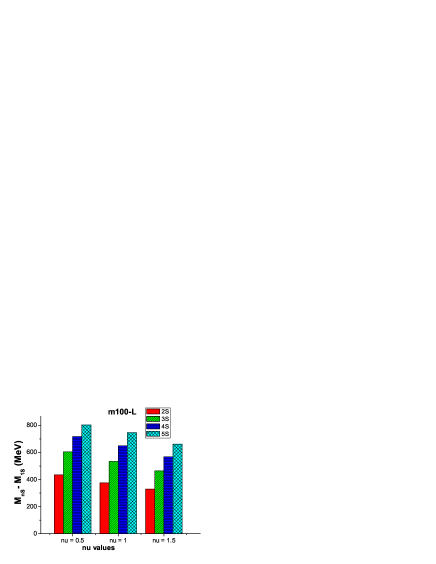
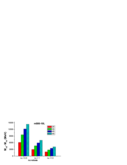
Figure 1: Comparative plot of the $nS$ energy levels w.r.t. the $1S$ state, taken as the ground level, found with the CpL and CpP potentials ($\nu=1,0.5,1.5$ respectively) for different $m_{Q}$ and $\Lambda$ values: m100 and m500 stands for the quirk mass value. L, 10L denotes $\Lambda=(1,10)\ \Lambda_{QCD}$, respectively.

In order to compare the effect of the above mentioned potentials, in Figure 1 we plot the $nS$ level spacings $\Delta_{nS-1S}=M(nS)-M(1S)$ of quirkonium found with the CpL and CpP potentials ($\nu=1,0.5,1.5$ respectively) for different $m_{Q}$ and $\Lambda$ values. As far as we are interested in disentangling peaks of $S$-wave resonances, it becomes apparent that this would be only possible in some cases (i.e. $\Lambda=\ 10\ \Lambda_{QCD}$) where the level spacing is ${\cal O}(1)$ GeV or larger.

II.3 Other possible contributions from short distance potential

Finally, to take into account other contributions which could be entangled in the short distance part of the potential, we consider higher (non perturbative) $\bar{\alpha^{\prime}}$ effective values. In order to consider this scenario, we do not use the Eq.(6) for $\alpha^{\prime}$ but we take it as a free parameter. On the other hand we keep the explicit dependence of $\Lambda$ ( Eq.(5) ) in $\sigma$. In this case we also increase the $\Lambda$ values from $\Lambda=\ 10\cdot\Lambda_{QCD}$ up to $\Lambda=\ 40\cdot\Lambda_{QCD}$.

By using QQ-onia code we find the results with $m_{Q}=500$ GeV for the mass level spacing $\Delta_{2S-1S}=M(2S)-M(1S)$ which are shown in Table 15 (Appendix). As we can see from these situations, we find separation between levels tens of GeV, thus, in principle, we should be able to discriminate at least between these resonances.

II.4 WFO vs. quirk masses.

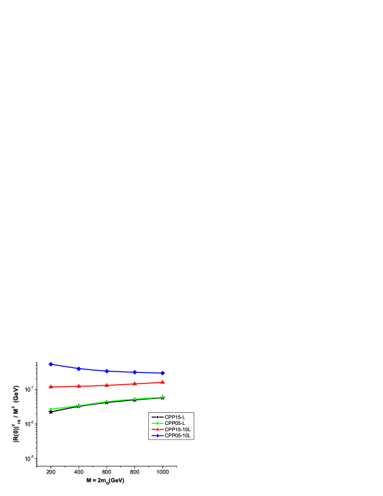
Figure 2: Values of $|R_{1S}(0)|^{2}/M^{2}$ (in $GeV$) corresponding to the $1S$ level vs. $M=2m_{Q}$ (in $GeV$) using CpP potentials with $\nu=0.5;1.5$ (labeled as CPP05, CPP15 respectively). L, 10L denote $\Lambda=(1,10)\ \Lambda_{QCD}$, respectively. The curve corresponding to $\nu=1$ lies in between.

Next let us analyze the WFO dependence w.r.t. the quirk mass using the above explained CpP potentials. Here we focus on the $1S$ ground level, by taking quirk mass values from $m_{Q}=100\ GeV$ up to $500\ GeV$. Again we will take $\Lambda=\ \Lambda_{QCD},\ 10\ \Lambda_{QCD}$ for each potential. For intermediate $m_{Q}$ values $\sigma$ does not change w.r.t. the mass values, However here $\alpha^{\prime}(Q=2m_{Q})$ changes for each case according to Eq.(6). Figure 2 displays the obtained results.

III Quirkonium decay

Once computed the squared WFO, we can evaluate numerically the partial decay widths of neutral (${}^{3}S_{1}$) quirkonium ($\psi_{Q\bar{Q}}$) to different final states. All of them are proportional to the ratio $|R_{S}(0)|^{2}/M^{2}$, where $M$ is the quirkonium mass. Subsequently we make estimates of the respective branching ratios ($BR$).

We will follow a similar treatment as the authors of cheung ,barger who considered the following $\psi_{Q\bar{Q}}$ decay modes:

• Decay to Standard Model fermion pairs ($f\bar{f}\equiv$leptons and quarks)

  $$\Gamma(\psi_{Q\bar{Q}}\longrightarrow f\bar{f})=F^{f\bar{f}}_{1}(N_{IC},R_{i},e_{Q},SM)\frac{|R_{S}(0)|^{2}}{M^{2}}$$ (7)

  where $F^{f\bar{f}}_{1}(N_{IC},R_{i},e_{Q},SM)$ stands for functions containing the i-colour number, squared mass ratios $R_{i}=M^{2}_{i}/M^{2}(i=f,Z)$ , the quirk electric charge $e_{Q}$. The $SM$ label means that those SM parameters involved in this calculation parameters are included.

• Decay to a $W^{\pm}$ pair

  $$\Gamma(\psi_{Q\bar{Q}}\longrightarrow W^{+}W^{-})=F_{2}(N_{IC},R_{i},SM)\frac{|R_{S}(0)|^{2}}{M^{2}}$$ (8)

  Where $F_{2}(N_{IC},R_{i},e_{Q},SM)$ stands for a function entangling the i-colour number, squared mass ratios $R_{i}=M^{2}_{i}/M^{2}(i=W,\ Z,\ m_{Q})$, and $SM$ parameters.

• Decay to i-gluons ($g^{\prime}$). Quirks couple to the i-gluon field of the $SU(N_{IC})$ with coupling strength $g_{s}^{\prime}=\sqrt{4\pi\alpha_{s}^{\prime}}$, where $\alpha_{s}^{\prime}(Q^{2})$ is given by Eq.(6).

  $$\Gamma(\psi_{Q\bar{Q}}\longrightarrow g^{\prime}g^{\prime}g^{\prime})=F_{3}(N^{2}_{IC},\alpha^{\prime 3})\frac{|R_{S}(0)|^{2}}{M^{2}}$$ (9)

  Here, $F_{3}(N^{2}_{IC},\alpha^{\prime 3})$ is a function of the i-colour number and the i-colour $\alpha^{\prime}$ coupling.

  $$\Gamma(\psi_{Q\bar{Q}}\longrightarrow\gamma\ g^{\prime}g^{\prime})=F_{4}(N_{IC},e^{2}_{Q},\alpha^{\prime 2})\frac{|R_{S}(0)|^{2}}{M^{2}}$$ (10)

  $$\Gamma(\psi_{Q\bar{Q}}\longrightarrow Z\ g^{\prime}g^{\prime})=F_{5}(N_{IC},e^{2}_{Q},\alpha^{\prime 2},SM)\frac{|R_{S}(0)|^{2}}{M^{2}}$$ (11)

To make the reading easy, the explicit form of $F_{i}(i=1,...,5)$ coefficients can be found in references cheung ,barger .

III.1 Numerical results

Once set the numerical values of parameters in the above expressions, the $|R_{S}(0)|^{2}$ values from Tables 1 to 14 (appendix) allow one to compute the decay widths of $\psi_{Q\bar{Q}}(1S)$ to $SM$ quarks ($q\bar{q}\equiv\ u\bar{u},\ d\bar{d},\ s\bar{s},\ c\bar{c},\ b\bar{b}$, [$t\bar{t}$ if above the threshold]), leptons ($\ell\bar{\ell}\equiv e^{\pm},\ \mu^{\pm},\ \tau^{\pm}$), and other boson decays ($W^{\pm},\ 3g^{\prime},\ \gamma 2g^{\prime},\ Z2g^{\prime}$). The results are shown in Table 16 for CpL and CpP (with $\nu=0.5,1.5$) potential using $m_{Q}=100\ GeV$ and $m_{Q}=500\ GeV$ at the above considered scales.

In all cases the decay mode to $SM$ quarks is the dominant channel. Decay to leptons shares roughly with a $33\%$ for electron, muon and $\tau$ pair respectively. As we can see, for $\Lambda=\Lambda_{QCD}$ case if we take into account only the $1S$ decay, the total width is quite narrow $\sim$KeV, but we find similar values than in the heavy quarkonia case pdg . For $\Lambda=10\Lambda_{QCD}$ case the total width increases roughly one order of magnitude. Nevertheless, if necessary, this analysis could be improved by adding upper $nS$ levels contributions: for instance if we compute the whole $nS$ contribution using the $m_{q}=500GeV;\ \Lambda=10\Lambda_{QCD}$ case, with a CpL potential we find a total width $\approx 1.7$ times the $1S$ total width; using CpP $\nu=1.5$ and $\nu=0.5$ potentials we find a factor $\approx 1.5$ and $\approx 2.$ respectively.

Concerning $P$-wave resonances ($l\neq 0$), the corresponding widths satisfy

$$\Gamma_{nP}\propto\frac{|R^{\prime}_{S}(0)|^{2}}{M^{4}}$$ (12)

so that, those contributions are suppressed with respect to the $nS$ decays by a (D) factor

$$\textsl{D}=\frac{1}{M^{2}}\ \frac{|R^{\prime}_{P}(0)|^{2}}{|R_{S}(0)|^{2}}$$

Taking $n=1$ values in the CpL case from Tables , we find $\textsl{D}\sim[10^{-5},10^{-4}]$ in the $m_{Q}=100\ GeV$ case and $\textsl{D}\sim[10^{-6},10^{-5}]$ for $m_{Q}=500\ GeV$. Regarding the dependence of the BRs on the quirk mass ($BR$ are independent of the ratio $|R_{S}(0)|^{2}/M^{2}$, but $M$ enters also thorugh the functions $F_{i}$): in the range of interest $100\leq m_{Q}\leq 500GeV$ we find variations on the different $BR$ less than a $1\%$.

We can also check the $BR$ variations with the i-colour number $N_{IC}$: by replacing for instance in the above expressions $N_{IC}=6\leftrightarrow N_{IC}=3\leftrightarrow N_{IC}=1$, the $BR$ to bosons varies mainly $33\%\leftrightarrow 17\%\leftrightarrow 5\%$ and the corresponding $BR$ to $SM$ quarks $55\%\leftrightarrow 68\%\leftrightarrow 78\%$ ($BR$ to leptons $12\%\leftrightarrow 15\%\leftrightarrow 17\%$ respectively).

IV Conclusions

Spectroscopy of exotic states might play a fundamental role in the discovery strategy of new physics at the LHC and ILC. In this paper we have focused on a simple extension of the SM, when a new $SU(N_{i})$ gauge group is added to the SM. The new interaction and new associated fermions have been dubbed i-color, quirks respectively. We assume that quirks are colorless, but otherwise carry SM quantum numbers, thereby coupling to gauge $W^{\pm},Z$ and $\gamma$ bosons.

Quirks can bind forming very peculiar structures reminding. In this work we have focused on neutral $Q\bar{Q}$ states called quirkonium, when the states are microscopic. We have performed a prospective study of quirkonium spectroscopy by employing a Coulomb plus Linear and Coulomb plus Power Law potentials as representative possibilities with parameters according to i-QCD requirements, as well as other effective contributions to analyze their impact.

Taking into account the wide range where the $Q\bar{Q}$ bound state might be found, we have chosen the scale range, MeV $\lesssim\Lambda\lesssim$ GeV with different i-colour $\Lambda$ scales and quirk masses, finding sizes of several $Q\bar{Q}_{nl}$ resonances and their squared WFO values of states (or derivatives for $l\neq 0$). We also extracted the level spacing among resonances using different $\Lambda$ scenarios to determine whether or not it would be possible to discriminate different state levels. We also have computed total and partial decay widths.

V Appendix: Tables

Table 1: Mass level spacings with respect to the ground state: $\Delta_{nl-1S}=M(nl)-M(1S)$ (MeV), using a Coulomb plus linear potential with $m_{Q}=100$ GeV; $\Lambda=0.1\cdot\Lambda_{QCD}=25$ MeV; $|R_{nl}^{(l)}(0)|^{2}/M^{(2+2l)}$ (in GeV), and mean square radius (in fm).

$Q\bar{Q}$ LEVEL	$\Delta_{nl-1S}$ (MeV)	$|R_{nl}^{(l)}(0)|^{2}/M^{(2+2l)}$	$\sqrt{\langle r^{2}\rangle}$
$(1S)$	$0$	$0.0092$	$0.06$
$(1P)$	$153$	$5.2\ 10^{-8}$	$0.23$
$(2S)$	$154$	$0.0012$	$0.28$
$(1D)$	$183$	$5.9\ 10^{-12}$	$0.45$
$(2P)$	$184$	$2.1\ 10^{-8}$	$0.54$
$(3S)$	$185$	$4.1\ 10^{-4}$	$0.58$
$(4S)$	$198$	$2.2\ 10^{-4}$	$0.93$
$(5S)$	$206$	$1.6\ 10^{-4}$	$1.27$

$\langle v^{2}\rangle\approx 10^{-4}$

Table 2: The same as in Table 1 for a CpL potential with $m_{Q}=100$ GeV; $\Lambda=0.4\cdot\Lambda_{QCD}=100$ MeV.

$Q\bar{Q}$ LEVEL	$\Delta_{nl-1S}$ (MeV)	$|R_{nl}^{l}(0)|^{2}/M^{(2+2l)}$	$\sqrt{\langle r^{2}\rangle}$
$(1S)$	$0$	$0.016$	$0.05$
$(1P)$	$229$	$1.7\ 10^{-7}$	$0.17$
$(2S)$	$234$	$0.0025$	$0.21$
$(1D)$	$288$	$8.3\ 10^{-11}$	$0.28$
$(2P)$	$297$	$1.1\ 10^{-7}$	$0.34$
$(3S)$	$302$	$0.0013$	$0.37$
$(4S)$	$344$	$9.5\ 10^{-4}$	$0.52$
$(5S)$	$377$	$7.9\ 10^{-4}$	$0.65$

$\langle v^{2}\rangle\approx[10^{-4},10^{-3}]$

Table 3: The same as in Table 1 for a CpL potential with $m_{Q}=100$ GeV; $\Lambda=\Lambda_{QCD}=250\ MeV$.

$Q\bar{Q}$ LEVEL	$\Delta_{nl-1S}$ (MeV)	$|R_{nl}^{l}(0)|^{2}/M^{(2+2l)}$	$\sqrt{\langle r^{2}\rangle}$
$(1S)$	$0$	$0.025$	$0.04$
$(1P)$	$348$	$6.6\ 10^{-7}$	$0.12$
$(2S)$	$375$	$0.0059$	$0.15$
$(1D)$	$473$	$7.0\ 10^{-10}$	$0.18$
$(2P)$	$508$	$6.0\ 10^{-7}$	$0.21$
$(3S)$	$533$	$0.0038$	$0.24$
$(4S)$	$649$	$0.0031$	$0.32$
$(5S)$	$746$	$0.0027$	$0.38$

$\langle v^{2}\rangle\approx 10^{-3}$

Table 4: The same as Table 1 for a CpL potential with $m_{Q}=100$ GeV; $\Lambda=\ 10\cdot\Lambda_{QCD}=2.5$ GeV.

$Q\bar{Q}$ LEVEL	$\Delta_{nl-1S}$ (GeV)	$|R_{nl}^{l}(0)|^{2}/M^{(2+2l)}$	$\sqrt{\langle r^{2}\rangle}$
$(1S)$	$0$	$0.218$	$0.02$
$(1P)$	$2.51$	$1.5\ 10^{-4}$	$0.03$
$(2S)$	$3.42$	$0.129$	$0.04$
$(1D)$	$4.15$	$3.1\ 10^{-7}$	$0.045$
$(2P)$	$5.03$	$2.1\ 10^{-4}$	$0.05$
$(3S)$	$5.84$	$0.109$	$0.06$
$(4S)$	$7.88$	$0.099$	$0.08$
$(5S)$	$9.70$	$0.092$	$0.09$

$\langle v^{2}\rangle\approx 10^{-2}$

Table 5: The same as in Table 1 for a CpL potential with $m_{Q}=500$ GeV; $\Lambda=\ \Lambda_{QCD}=250$ MeV.

$Q\bar{Q}$ LEVEL	$\Delta_{nl-1S}$ (MeV)	$|R_{nl}^{l}(0)|^{2}/M^{(2+2l)}$	$\sqrt{\langle r^{2}\rangle}$
$(1S)$	$0$	$0.058$	$0.008$
$(1P)$	$831$	$4.5\ 10^{-7}$	$0.04$
$(2S)$	$850$	$0.0063$	$0.05$
$(1D)$	$1028$	$2.0\ 10^{-11}$	$0.07$
$(2P)$	$1042$	$2.3\ 10^{-7}$	$0.09$
$(3S)$	$1054$	$0.0026$	$0.1$
$(4S)$	$1162$	$0.0017$	$0.15$
$(5S)$	$1239$	$0.0013$	$0.19$

$\langle v^{2}\rangle\approx 10^{-4}$

Table 6: The same as in Table 1 for a CpL potential with $m_{Q}=500$ GeV, $\Lambda=\ 10\cdot\Lambda_{QCD}=2.5$ GeV.

$Q\bar{Q}$ LEVEL	$\Delta_{nl-1S}$ (GeV)	$|R_{nl}^{l}(0)|^{2}/M^{(2+2l)}$	$\sqrt{\langle r^{2}\rangle}$
$(1S)$	$0$	$0.187$	$0.007$
$(1P)$	$2.44$	$1.0\ 10^{-5}$	$0.017$
$(2S)$	$2.98$	$0.048$	$0.022$
$(1D)$	$3.71$	$2.0\ 10^{-9}$	$0.024$
$(2P)$	$4.18$	$2.0\ 10^{-5}$	$0.029$
$(3S)$	$4.64$	$0.0350$	$0.033$
$(4S)$	$5.96$	$0.030$	$0.042$
$(5S)$	$7.11$	$0.027$	$0.051$

$\langle v^{2}\rangle\approx 10^{-3}$

Table 7: The same as in table 1 for Coulomb plus power law potential with $\nu=0.5$, $m_{Q}=100$ GeV; $\Lambda=\ \Lambda_{QCD}=250$ MeV.

$Q\bar{Q}$ LEVEL	$\Delta_{nl-1S}$ (MeV)	$|R_{nl}^{l}(0)|^{2}/M^{(2+2l)}$	$\sqrt{\langle r^{2}\rangle}$
$(1S)$	$0$	$0.027$	$0.05$
$(1P)$	$400$	$9.6\ 10^{-7}$	$0.11$
$(2S)$	$434$	$0.0068$	$0.14$
$(1D)$	$545$	$6.7\ 10^{-11}$	$0.17$
$(2P)$	$579$	$7.6\ 10^{-7}$	$0.21$
$(3S)$	$604$	$0.0039$	$0.23$
$(4S)$	$717$	$0.0029$	$0.32$
$(5S)$	$803$	$0.0023$	$0.41$

$\langle v^{2}\rangle\approx 10^{-3}$

Table 8: The same as in Table 1 for a CpP potential with $\nu=0.5$, $m_{Q}=500$ GeV; $\Lambda=\ \Lambda_{QCD}=250$ MeV.

$Q\bar{Q}$ LEVEL	$\Delta_{nl-1S}$ (MeV)	$|R_{nl}^{l}(0)|^{2}/M^{(2+2l)}$	$\sqrt{\langle r^{2}\rangle}$
$(1S)$	$0$	$0.060$	$0.01$
$(1P)$	$880$	$5.6\ 10^{-7}$	$0.04$
$(2S)$	$911$	$0.0072$	$0.05$
$(1D)$	$1112$	$6.0\ 10^{-12}$	$0.07$
$(2P)$	$1132$	$3.0\ 10^{-7}$	$0.08$
$(3S)$	$1150$	$0.0031$	$0.09$
$(4S)$	$1276$	$0.0020$	$0.14$
$(5S)$	$1363$	$0.0015$	$0.18$

$\langle v^{2}\rangle\approx 10^{-4}$

Table 9: The same as in Table 1 for a CpP potential with $\nu=0.5$, $m_{Q}=100$ GeV; $\Lambda=\ 10\cdot\Lambda_{QCD}=2.5$ GeV.

$Q\bar{Q}$ LEVEL	$\Delta_{nl-1S}$ (GeV)	$|R_{nl}^{l}(0)|^{2}/M^{(2+2l)}$	$\sqrt{\langle r^{2}\rangle}$
$(1S)$	$0$	$0.539$	$0.014$
$(1P)$	$5.09$	$6.3\ 10^{-4}$	$0.024$
$(2S)$	$6.94$	$0.298$	$0.031$
$(1D)$	$8.36$	$3.1\ 10^{-6}$	$0.032$
$(2P)$	$9.84$	$0.0013$	$0.040$
$(3S)$	$11.28$	$0.227$	$0.046$
$(4S)$	$14.63$	$0.190$	$0.060$
$(5S)$	$17.42$	$0.167$	$0.073$

$\langle v^{2}\rangle\approx 10^{-2}$

Table 10: The same as in Table 1 for a CpP potential with $\nu=0.5$, $m_{Q}=500$ GeV; $\Lambda=\ 10\cdot\Lambda_{QCD}=2.5$ GeV.

$Q\bar{Q}$ LEVEL	$\Delta_{nl-1S}$ (GeV)	$|R_{nl}^{l}(0)|^{2}/M^{(2+2l)}$	$\sqrt{\langle r^{2}\rangle}$
$(1S)$	$0$	$0.298$	$0.007$
$(1P)$	$4.60$	$9.0\ 10^{-5}$	$0.012$
$(2S)$	$6.14$	$0.107$	$0.015$
$(1D)$	$7.39$	$5.0\ 10^{-8}$	$0.016$
$(2P)$	$8.44$	$1.0\ 10^{-4}$	$0.020$
$(3S)$	$9.61$	$0.075$	$0.023$
$(4S)$	$12.21$	$0.061$	$0.031$
$(5S)$	$14.33$	$0.052$	$0.038$

$\langle v^{2}\rangle\approx 10^{-3}$

Table 11: The same as in Table 1 for a CpP potential with $\nu=1.5$, $m_{Q}=100$ GeV; $\Lambda=\ \Lambda_{QCD}=250$ MeV.

$Q\bar{Q}$ LEVEL	$\Delta_{nl-1S}$ (MeV)	$|R_{nl}^{l}(0)|^{2}/M^{(2+2l)}$	$\sqrt{\langle r^{2}\rangle}$
$(1S)$	$0$	$0.022$	$0.05$
$(1P)$	$313$	$4.6\ 10^{-7}$	$0.13$
$(2S)$	$329$	$0.0049$	$0.16$
$(1D)$	$416$	$1.5\ 10^{-11}$	$0.20$
$(2P)$	$445$	$4.4\ 10^{-7}$	$0.23$
$(3S)$	$464$	$0.0034$	$0.25$
$(4S)$	$568$	$0.0029$	$0.33$
$(5S)$	$662$	$0.0027$	$0.39$

$\langle v^{2}\rangle\approx 10^{-3}$

Table 12: The same as in Table 1 for a CpP potential $\nu=1.5$, $m_{Q}=500$ GeV; $\Lambda=\ \Lambda_{QCD}=250$ MeV.

$Q\bar{Q}$ LEVEL	$\Delta_{nl-1S}$ (MeV)	$|R_{nl}^{l}(0)|^{2}/M^{(2+2l)}$	$\sqrt{\langle r^{2}\rangle}$
$(1S)$	$0$	$0.058$	$0.01$
$(1P)$	$813$	$3.7\ 10^{-7}$	$0.04$
$(2S)$	$827$	$0.0058$	$0.05$
$(1D)$	$991$	$2.0\ 10^{-12}$	$0.08$
$(2P)$	$998$	$1.8\ 10^{-7}$	$0.10$
$(3S)$	$1005$	$0.0022$	$0.11$
$(4S)$	$1094$	$0.0015$	$0.16$
$(5S)$	$1198$	$0.0011$	$0.20$

$\langle v^{2}\rangle\approx 10^{-4}$

Table 13: The same as in Table 1 for a CpP potential with $\nu=1.5$, $m_{Q}=100$ GeV; $\Lambda=\ 10\cdot\Lambda_{QCD}=2.5$ GeV.

$Q\bar{Q}$ LEVEL	$\Delta_{nl-1S}$ (GeV)	$|R_{nl}^{l}(0)|^{2}/M^{(2+2l)}$	$\sqrt{\langle r^{2}\rangle}$
$(1S)$	$0$	$0.118$	$0.027$
$(1P)$	$1.12$	$4.1\ 10^{-5}$	$0.041$
$(2S)$	$1.88$	$0.067$	$0.057$
$(1D)$	$2.33$	$3.1\ 10^{-8}$	$0.060$
$(2P)$	$2.83$	$5.8\ 10^{-5}$	$0.070$
$(3S)$	$3.27$	$0.059$	$0.079$
$(4S)$	$4.52$	$0.056$	$0.097$
$(5S)$	$5.69$	$0.054$	$0.112$

$\langle v^{2}\rangle\approx 10^{-2}$

Table 14: The same as in Table 1 for a CpP potential with $\nu=1.5$, $m_{Q}=500$ GeV; $\Lambda=\ 10\cdot\Lambda_{QCD}=2.5$ GeV.

$Q\bar{Q}$ LEVEL	$\Delta_{nl-1S}$ (GeV)	$|R_{nl}^{l}(0)|^{2}/M^{(2+2l)}$	$\sqrt{\langle r^{2}\rangle}$
$(1S)$	$0$	$0.160$	$0.008$
$(1P)$	$1.73$	$5.0\ 10^{-6}$	$0.023$
$(2S)$	$1.91$	$0.026$	$0.029$
$(1D)$	$2.04$	$8.0\ 10^{-10}$	$0.031$
$(2P)$	$2.62$	$5.0\ 10^{-6}$	$0.040$
$(3S)$	$2.80$	$0.019$	$0.044$
$(4S)$	$3.51$	$0.016$	$0.057$
$(5S)$	$4.15$	$0.015$	$0.067$

$\langle v^{2}\rangle\approx 10^{-3}$

Table 15: Mass level spacing $\Delta_{2S-1S}=M(2S)-M(1S)$ (with $m_{Q}=500$ GeV) using $\Lambda=(10,20,40)\cdot\Lambda_{QCD}$ and different $\bar{\alpha^{\prime}}$ values.

$\Lambda$	$\bar{\alpha^{\prime}}$	$\Delta_{2S-1S}$ (GeV)
$10\cdot\Lambda_{QCD}$	$0.3$	$\approx 10$
$20\cdot\Lambda_{QCD}$	$0.3$	$\approx 12$
$40\cdot\Lambda_{QCD}$	$0.6$	$\approx 30$

Table 16: Branching Ratios of $\psi_{Q\bar{Q}}(1S)\ (M=\ 2m_{Q}=\ 200\ GeV)$ and $\psi_{Q\bar{Q}}(1S)\ (M=1000\ GeV)$ to $SM$ quarks ($q\bar{q}$),leptons ($l\bar{l}$), and other boson decays. $\Gamma$(CpL,CpP15,CpP05) stands for the total decay width (in $KeV$) using each potential.

$\psi_{Q\bar{Q}}(1S)\ (M=200\ GeV)$
$\Lambda(MeV)$	$\Gamma$(CpL,CpP15,CpP05)$(KeV)$	$BR(l\bar{l})(\%)$	$BR(q\bar{q})(\%)$	$BR(Boson)(\%)$
$25$	$(31,--,--)$	$17$	$76$	$7$
$100$	$(54,--,--)$	$16$	$76$	$8$
$250$	$(86,\ 78,\ 94)$	$16$	$75$	$9$
$2500$	$(833,451,2060)$	$15$	$68$	$17$
$\psi_{Q\bar{Q}}(1S)\ (M=1000\ GeV)$
$\Lambda(MeV)$	$\Gamma$(CpL,CpP15,CpP05)$(KeV)$	$BR(l\bar{l})(\%)$	$BR(q\bar{q})(\%)$	$BR(Boson)(\%)$
$250$	$(165,164,169)$	$16$	$80$	$4$
$2500$	$(555,474,882)$	$16$	$76$	$8$