Dynamics of the the dihedral four-body problem

Abstract

Consider four point particles with equal masses in the euclidean space, subject to the following symmetry constraint: at each instant they are symmetric with respect to the dihedral group $D_{2}$, that is the group generated by two rotations of angle $\pi$ around two orthogonal axes. Under a homogeneous potential of degree $-\alpha$ for $0<\alpha<2$, this is a subproblem of the four-body problem, in which all orbits have zero angular momentum and the configuration space is three-dimensional. In this paper we study the flow in McGehee coordinates on the collision manifold, and discuss the qualitative behavior of orbits which reach or come close to a total collision.

MSC Subject Class: Primary 70F10; Secondary 37C80. Keywords: Dihedral $4$-body problem, McGehee coordinates, heteroclinics.

1 Introduction

The goal of this paper is to investigate the qualitative behavior of solutions of the dihedral symmetric $4$-body problem in space under the action of a homogeneous potential of degree $-\alpha$. For the Newtonian potential this problem is a kind of generalization of Devaney planar isosceles three body problem [Dev80, Dev81], following Moeckel’s approach to the study of the three body problem in space [Moe81, Moe83]. The dihedral four-body problem is a subproblem of the full four-body problem which reduces to a three-dimensional configuration space. Briefly, one takes $n=4$ equal masses whose initial position and velocity are symmetric with respect to the $2$-dihedral group (which is isomorphic to the Klein group $\mathbb{Z}_{2}\times\mathbb{Z}_{2}$) $D_{2}\subset SO(3)$. So the masses form a (possibly planar, degenerate and non-regular) tetrahedron in space. Because of the symmetry of the problem, the masses will remain in such a configuration for all time. Hence we have a system with only three degrees of freedom.

We will use McGehee coordinates [McG74] in order to study the dynamics of the dihedral four body problem for a general homogeneous potential of degree $-\alpha$ and with a slight change: we consider McGehee coordinates not only for studying the behavior of solutions passing close to a total collision, but also for parabolic orbits connecting central configurations, projecting the full phase space to a codimension $1$ subspace. We replace the singularity due to total collapse with an invariant immersed manifold in the full phase space usually called total collision manifold which is the immersion of the parabolic manifold of the projected phase space. By studying this flow we are able to establish some global results on the behavior of solutions. We discuss the qualitative behavior of orbits which reach or come close to the total collision and the behavior of orbits which start from total collapse, which implies chaotic behavior. Such of problem includes a some of other subsystems with one or two degrees of freedom studied in the past years. We also observe that the behavior of the bodies is the same for all values of the parameters $\alpha\in(0,2)$ and not only for the Newtonian case $\alpha=1$.

The literature on this problem is quite broad and for this we quote just few papers in which similar studies were carried over. In particular some properties of the behavior of the flow on the total collision manifold has been established for the planar case in [SL82]. Moreover, in the spatial case in a series of papers Delgado and Vidal in [DV99, Vid99] studied the so-called tetrahedral four body problem without and with rotation. We observe that the potential in this case (up to a multiplicative constant depending on the normalization of the masses) coincides with a subcase of the dihedral four body problem.

The main results are presented in the first part of the article, in sections 2, 3 and 4, where we introduce the parabolic flow on the collision manifold for the 2-dihedral four-body problem, we prove the existence or non-existence of parabolic trajectories connecting rest points or singular sets, and then analyze the consequences on orbits close to total collision via topological transversality. Many tedious computations are postponed to the appendix.

2 Blow up, regularization and total collision manifold

We set ${\bf n}:=\{1,\dots,n\}$. Let $V:=\mathbb{R}^{d}$ denote the Euclidean space of dimension $d$ and $n\geq 2$ an integer, and denote with $\bm{0}$ the origin in $\mathbb{R}^{d}$. Given $n$ point mass particles in $V$ $P_{k}$, $k\in{\bf n}$ with positions ${\bm{q}}_{k}$, momenta ${\bm{p}}_{k}$ and masses $m_{k}\in\mathbb{R}^{+}$, let ${\bm{q}},{\bm{p}}\in V^{n}$ be the vectors $({\bm{q}}_{1},\dots,{\bm{q}}_{n})$, $({\bm{p}}_{1},\dots\bm{p}_{n})$. Let $\alpha>0$ be a given positive real number. We consider the potential function (the opposite of the potential energy) defined by

$$\sum_{i<j}\dfrac{m_{i}m_{j}}{|{\bm{q}}_{i}-{\bm{q}}_{j}|^{\alpha}}.$$

If $M$ denotes the mass matrix namely the diagonal $nd\times nd$ matrix given by

$$M:=\mathrm{diag}(\underbrace{m_{1},\dots,m_{1}}_{\textrm{$d$ times}},\dots,\overbrace{m_{n}\dots m_{n}}_{\textrm{$d$ times}})$$

then Newton equations

$$M\ddot{\bm{q}}=\dfrac{\partial U}{\partial{\bm{q}}}$$

can be written in Hamiltonian form as

(1) $$\left\{\begin{aligned} M\dot{\bm{q}}&={\bm{p}}\\ \dot{\bm{p}}&=\dfrac{\partial U}{\partial{\bm{q}}},\end{aligned}\right.$$

where the Hamiltonian (i.e. the energy) is $H=H({\bm{q}},{\bm{p}})=\langle\dfrac{1}{2}M^{-1}{\bm{p}},{\bm{p}}\rangle-U({\bm{q}})$. Here we denoted by

$$\dfrac{\partial}{\partial{\bm{q}}}:=\left(\dfrac{\partial}{\partial{\bm{q}}_{1}},\dots,\dfrac{\partial}{\partial{\bm{q}}_{n}}\right),\qquad\dfrac{\partial}{\partial{\bm{q}}_{j}}:=\left(\dfrac{\partial}{\partial{\bm{q}}_{j}^{1}},\dots,\dfrac{\partial}{\partial{\bm{q}}_{j}^{n}}\right).$$

We will assume that the center of mass and the linear momentum remains at the origin and we define

$${\bm{Q}}=\{{\bm{q}}=({\bm{q}}_{1},\dots,{\bm{q}}_{n})\in V^{n}|\sum_{i=1}^{n}m_{i}{\bm{q}}_{i}=\bm{0}\},\ \ {\bm{P}}=\{{\bm{p}}=({\bm{p}}_{1},\dots,{\bm{p}}_{n})\in V^{n}|\sum_{i=1}^{n}{\bm{p}}_{i}=\bm{0}\}.$$

For each pair of indexes $i,j\in{\bf n}$ let $\Delta_{i,j}$ denote the collision set of the $i$-th and $j$-th particles $\Delta_{i,j}=\{{\bm{q}}\in{\bm{Q}}|{\bm{q}}_{i}={\bm{q}}_{j}\}$. For $i\neq j$, let $\Delta=\bigcup_{i,j}\Delta_{i,j}$ be the collision set in ${\bm{Q}}$. The set of collision-free configurations is denoted by $\hat{\bm{Q}}={\bm{Q}}\backslash\Delta$. The differential equations (1) then determine a vectorfield with singularities on $V^{n}\times V^{n}$, or a real analytic vectorfield without singularities on $(V^{n}\setminus\Delta)\times V^{n}$. The vectorfield given by (1) is everywhere tangent to ${\bm{Q}}\times{\bm{P}}$ and so this $2d(n-1)$ dimensional linear subspace is invariant under the flow. We henceforth restrict our attention to the flow on the phase space ${\bm{Q}}\times{\bm{P}}$. Consequently, $H$ is an integral of the system. This means that the level sets $\Sigma_{e}:=H^{-1}(e)\cap({\bm{Q}}\times{\bm{P}})$ are also invariant under the flow (1). We observe that $\Sigma_{e}$ is a real analytic submanifold of $({\bm{Q}}-\Delta)\times{\bm{P}}$ having dimension $2d(n-1)-1$ and the flow is not complete, however. In fact certain solutions run off in finite time; this happens exactly in correspondence to certain initial conditions leading to a collision between two or more particles and the corresponding solution curve meet $\Delta$ in finite time. Since we are interested primarily in solution curves leading to total collapse and since the center of mass is fixed at the origin, this must occur at the origin of ${\bm{Q}}$.

2.1 McGehee coordinates

The aim of this section is to recall McGehee coordinates as given in [FP08] in order to fix notations. Our basic reference will be [FP08] and references therein.

The equations (1) can be written in polar coordinates by setting the mass norm in $V^{n}$ defined for every ${\bm{q}}\in V^{n}$ as

$$\left\|{\bm{q}}\right\|^{2}=\langle M{\bm{q}},{\bm{q}}\rangle$$

and suitably rescaling the momentum as follows

$$\rho=\left\|{\bm{q}}\right\|,\ {\bm{s}}=\dfrac{{\bm{q}}}{\rho},\ {\bm{z}}=\rho^{\beta}{\bm{p}}\qquad\qquad\text{with $\alpha=2\beta$.}$$

In these coordinates equations (1) can be read as

(2) $$\left\{\begin{aligned} \rho^{\prime}&=\langle{\bm{z}},{\bm{s}}\rangle\rho\\ {\bm{s}}^{\prime}&=M^{-1}{\bm{z}}-\langle{\bm{z}},{\bm{s}}\rangle{\bm{s}}\\ {\bm{z}}^{\prime}&=\beta\langle{\bm{z}},{\bm{s}}\rangle{\bm{z}}+\dfrac{\partial U}{\partial{\bm{q}}}({\bm{s}}),\end{aligned}\right.$$

where the time has been rescaled by $dt=\rho^{1+\beta}d\tau$ (that is, $\dfrac{d}{d\tau}=\rho^{1+\beta}\dfrac{d}{dt}$); now the energy can be written as

(3) $$H=\dfrac{1}{2}\rho^{-\alpha}\langle M^{-1}{\bm{z}},{\bm{z}}\rangle-\rho^{-\alpha}U({\bm{s}})=\rho^{-\alpha}\left(\dfrac{1}{2}\langle M^{-1}{\bm{z}},{\bm{z}}\rangle-U({\bm{s}})\right).$$

Let $k:=d(n-1)$ and let us consider the projection $({\bm{q}},{\bm{p}})\mapsto({\bm{s}},{\bm{z}})$ from the full phase space ${\bm{Q}}\times{\bm{P}}$ to the reduced space $S^{k-1}\times{\bm{P}}$ (which is the trivial $\mathbb{R}^{k}$-bundle on the shape sphere $S^{k-1}$)

$${\bm{Q}}\times{\bm{P}}\to S^{k-1}\times{\bm{P}}.$$

We define the parabolic manifold as the projection of all zero-energy orbits (or, equivalently, of the zero-energy submanifold of ${\bm{Q}}\times{\bm{P}}$) in $S\times{\bm{P}}$, where $\mathbb{S}=S^{k-1}$, that is

$${\mathscr{P}}=\{({\bm{s}},{\bm{z}})\in S\times{\bm{P}}:\dfrac{1}{2}\langle M^{-1}{\bm{z}},{\bm{z}}\rangle=U(s)\}\subset S^{k-1}\times{\bm{P}}.$$

The next change of coordinates, due to McGehee [McG74], is needed for defining the Sundman–Lyapunov coordinate $v$ and for the regularization of the parabolic manifold ${\mathscr{P}}$. Let $v,{\bm{w}}$ be defined by

$$\begin{cases}v&=\langle{\bm{z}},{\bm{s}}\rangle\\ {\bm{w}}&=M^{-1}{\bm{z}}-\langle{\bm{z}},{\bm{s}}\rangle{\bm{s}}.\end{cases}$$

Then ${\bm{z}}=vM{\bm{s}}+M{\bm{w}}$ and $\langle{\bm{w}},M{\bm{s}}\rangle=0$ (so that ${\bm{w}}$ is also tangent to $S$), and (2) can be replaced by

(4) $$\left\{\begin{aligned} \rho^{\prime}&=\rho v\\ v^{\prime}&=\left\|{\bm{w}}\right\|^{2}+\beta v^{2}-\alpha U({\bm{s}})\\ {\bm{s}}^{\prime}&={\bm{w}}\\ {\bm{w}}^{\prime}&=-\left\|{\bm{w}}\right\|^{2}{\bm{s}}+(\beta-1)v{\bm{w}}+M^{-1}\nabla_{{\bm{s}}}U({\bm{s}}),\end{aligned}\right.$$

where $\nabla_{{\bm{s}}}$ denotes covariant derivative associated to the Levi-Civita connection induced by the Riemannian metric $\langle\cdot,\cdot\rangle_{M}:=\langle M\cdot,\cdot\rangle$, i.e. the component of the gradient tangent to the inertia ellipsoid $\left\|{\bm{q}}\right\|=1$, i.e.

$$\nabla_{\bm{s}}U=\dfrac{\partial U}{\partial{\bm{q}}}({\bm{s}})+\alpha U({\bm{s}})M{\bm{s}}.$$

In fact

$$\langle M^{-1}\nabla_{\bm{s}}U({\bm{s}}),{\bm{v}}\rangle =\langle\dfrac{\partial U}{\partial{\bm{q}}}({\bm{s}}),{\bm{v}}\rangle+\alpha U({\bm{s}})\langle M{\bm{s}},{\bm{v}}\rangle=$$

$$=\langle\dfrac{\partial U}{\partial{\bm{q}}}({\bm{s}}),{\bm{v}}\rangle=dU({\bm{s}})[{\bm{v}}]=\langle M^{-1}\nabla_{\bm{s}}U({\bm{s}}),v\rangle_{M}$$

The energy relation becomes

$$2\rho^{\alpha}H=\|{\bm{w}}\|^{2}+\|v\|^{2}-2U({\bm{s}})$$

while the parabolic manifold ${\mathscr{P}}$ is then defined by the equation

$$v^{2}+\left\|{\bm{w}}\right\|^{2}=2U({\bm{s}}).$$

We observe that differential equation (4) gives a real analytic vectorfield with singularities on the manifold with boundary $\Omega:=(0,\infty)\times\mathbb{R}\times TS$; equivalently it defines a real analytic vectorfield without singularities on $[0,\infty)\times\mathbb{R}\times T(S\setminus\Delta)$.

In these coordinates the assumption about the center of mass gives:

(5) $${\bm{S}}=\{{\bm{s}}=({\bm{s}}_{1},\dots,{\bm{s}}_{n})\in V^{n}|\sum_{i=1}^{n}m_{i}{\bm{s}}_{i}=\bm{0}\},\ \ {\bm{W}}=\{{\bm{w}}=({\bm{w}}_{1},\dots,{\bm{w}}_{n})\in V^{n}|\sum_{i=1}^{n}m_{i}{\bm{w}}_{i}=\bm{0}\}.$$

Let ${\bm{M}}(h)$ denote the subset of $(\rho,{\bm{s}},{\bm{w}})$ defined as follows:

(6) $${\bm{M}}(h):=\left\{{(\rho,{\bm{s}},{\bm{w}})\in[0,\infty)\times\mathbb{S}\times{\bm{W}}}\mid{\eqref{eq:energy}-\eqref{eq:centerofmass}\ \textrm{hold}}\right\}.$$

Let ${\bm{M}}_{+}(h)$ and ${\bm{M}}_{0}$ denote the subsets satisfying $\rho>0$ and $\rho=0$ respectively. All three are invariant submanifolds for the vectorfield (2). Note ${\bm{M}}_{0}$ is independent of $h$. We shall refer to ${\bm{M}}_{0}$ as McGehee total collision manifold. We observe also that the parabolic manifold ${\mathscr{P}}$ introduced above actually is the projection of McGehee total collision manifold (see [McG74, Dev80, Moe81, Moe83]); the manifold of $({\bm{s}},{\bm{w}})$ here is not considered as embedded in the space of $(\rho,{\bm{s}},{\bm{w}})$ with $\rho=0$.

Remark 2.1

As already remarked by several authors the effect of these transformations and of the time scaling has the effect of gluing a boundary given by $\rho=0$ onto the phase space. Since $\rho^{\prime}=0$ when $\rho=0$, this boundary is invariant under the flow generated by (4).

By the second equation in (4) can be deduced the well-known fact that for $0<\alpha<2$, $v$ is a Lyapunov function on the flow in the parabolic manifold, and therefore the flow is dissipative (gradient-like). Moreover, the equilibrium points in (4) are the projections of the equilibrium points of (2) (and the projection is one-to-one in the parabolic manifold), which can be found as solutions of

(7) $$\left\{\begin{aligned} v^{2}&=2U({\bm{s}})\\ \nabla_{{\bm{s}}}U({\bm{s}})&=\bm{0}\\ {\bm{w}}&=\bm{0}.\end{aligned}\right.$$

Hence all equilibrium points belong to the parabolic manifold ${\mathscr{P}}$.

2.2 The linearized flow

As already observed in section before the vectorfield (4) has the equilibrium points given in (7); moreover as already observed all these points lie on the total collision manifold. We now turn our attention to the calculation of the characteristic exponents of the various equilibrium points in ${\bm{M}}_{0}$. Accordingly, let $\bar{\bm{s}}$ be a central configuration and let $\bar{v}=\sqrt{2U(\bar{\bm{s}})}$. Then using

(8) $$\left\{\begin{aligned} \rho^{\prime}&=\rho v\\ {\bm{s}}^{\prime}&={\bm{w}}\\ {\bm{w}}^{\prime}&=-\left\|{\bm{w}}\right\|^{2}{\bm{s}}+(\beta-1)v{\bm{w}}+M^{-1}\nabla_{{\bm{s}}}U({\bm{s}}),\end{aligned}\right.$$

one computes the characteristic exponents for the flow in ${\bm{M}}(h)$. To study the eigenvalues of the linearized vectorfield at a restpoint $\bar{\gamma}=(0,\bar{\bm{s}},0)$, we introduce coordinates $(\zeta_{\rho},\zeta_{\bm{s}},\zeta_{\bm{w}})$ in the tangent space to $\mathbb{R}^{2nd+1}$. Let ${\bm{g}}$ be the Riemannian manifold induced by $\mathbb{R}^{2nd+1}$ on the $[2d(n-1)-1]$-dimensional manifold ${\bm{M}}_{0}$, $D$ and $\dfrac{D}{dt}$ be respectively the Levi-Civita connection and the covariant derivative associated to the Riemannian metric ${\bm{g}}$. The linearization along an orbit $\gamma_{0}$ is represented in local chart by the linear autonomous system

(9) $$\frac{D}{dt}{\bm{\zeta}}(t)\,=\,{\bm{C}}\,{\bm{\zeta}}(t),\qquad\forall\,t\in\mathbb{R}$$

where ${\bm{\zeta}}\in\bar{\gamma}^{*}\big{(}T{\bm{M}}(h)\big{)}$ is the vector field along the curve $\bar{\gamma}$ and where the variational matrix $A$ is the block matrix represented by

(10) $${\bm{C}}:=\begin{pmatrix}\bar{v}&0&0\\ &&\\ 0&0&I\\ &&\\ 0&M^{-1}D\nabla_{\bm{s}}U(\bar{\bm{s}})&(\beta-1)\bar{v}\end{pmatrix}.$$

Devaney has observed that one can guess eigenvector for problem of this type. In fact, given the matrix below

(11) $${\bm{B}}=\begin{pmatrix}0&I\\ &\\ M^{-1}D\nabla_{\bm{s}}U(\bar{\bm{s}})&(\beta-1)\bar{v}\end{pmatrix}$$

and assuming that ${\bm{\xi}}$ is a $[d(n-1)-1]$-eigenvector of the matrix ${\bm{A}}:=M^{-1}D\nabla_{\bm{s}}U(\bar{\bm{s}})$ (the Hessian $D^{2}U({\bm{s}})$)associated to the eigenvalue $\lambda$, then the $[2d(n-1)-1]$-dimensional vector $\tilde{\bm{\xi}}=({\bm{\xi}},\mu{\bm{\xi}})^{T}$ satisfies the following:

$$\begin{pmatrix}0&I\\ &\\ {\bm{A}}&(\beta-1)\bar{v}\end{pmatrix}\begin{pmatrix}{\bm{\xi}}\\ &\\ \mu{\bm{\xi}}\end{pmatrix}=\begin{pmatrix}\mu\,{\bm{\xi}}\\ &\\ \lambda\,{\bm{\xi}}+(\beta-1)\bar{v}\mu\,{\bm{\xi}}\end{pmatrix}$$

By a straightforward calculation it follows that $\mu$ is an eigenvalue of ${\bm{B}}$ if

$$\mu^{2}+(1-\beta)\bar{v}\mu=\lambda,$$

namely

$$\mu_{1,2}=\dfrac{(\beta-1)\bar{v}\pm\sqrt{(\beta-1)^{2}\bar{v}^{2}+4\lambda}}{2}.$$

We observe that, in the Newtonian case corresponding to $\beta=1/2$ this formula agrees with that of [DV99]. By this we have the following result.

Proposition 2.2

All equilibrium points are hyperbolic.

Proof.  For the proof of this result, see [FP08, Proposition 3.8] $\Box\\$

Proposition 2.3

The dimension of the stable (unstable) manifold of $(\overline{v},\overline{\bm{s}},\bm{0})$ with $\overline{v}=\sqrt{2U(\overline{\bm{s}})}>0$ is 3 (2) if $\overline{\bm{s}}$ is a rectangle; it is 2 (3) if $\overline{\bm{s}}$ is a tetrahedron. The dimension of the stable (unstable) manifold of the point $(-\overline{v},\overline{\bm{s}},\bm{0})$ with $\overline{v}=\sqrt{2U(\overline{\bm{s}})}>0$ is equal to the dimension of the unstable (stable) manifold of $(\overline{v},\overline{\bm{s}},\bm{0})$. The intersection of the stable (unstable) manifold of $(\overline{v},\overline{\bm{s}},\bm{0})$ with the parabolic manifold ${\mathscr{P}}$ has codimension 0 (1) in ${\mathscr{P}}$ if $\overline{v}>0$. It has codimension 1 (0) in ${\mathscr{P}}$ if $\overline{v}<0$.

Proof.  For the proof of this result, see [FP08, Proposition 3.9] $\Box\\$

2.3 McGehee coordinates for the (anisotropic) Kepler problem

Consider the classical anisotropic Kepler problem, in which $S\subset\mathbb{R}^{2}$ is a $1$-dimensional manifold. Let $(0,2\pi)\to S$ be a (maybe partially defined) local parametrisation, which we will denote by $\theta\mapsto{\bm{s}}(\theta)$, where ${\bm{s}}(\theta)=(m_{1}^{-1/2}\cos\theta,m_{2}^{-1/2}\sin\theta)$, if $m_{1}$ and $m_{2}$ are the diagonal entries of $M$. If we introduce the vector $\hat{\bm{s}}=(-m_{1}^{-1/2}\sin\theta,m_{2}^{-1/2}\cos\theta)$ and the scalar $w$ such that ${\bm{w}}=w\hat{\bm{s}}$, then equations (4) turn out to become

(12) $$\left\{\begin{aligned} v^{\prime}&=w^{2}+\beta\left(v^{2}-2U(\theta)\right)\\ \theta^{\prime}&=w\\ w^{\prime}&=(\beta-1)vw+U^{\prime}(\theta),\end{aligned}\right.$$

where we use the primes for denoting the differentiation with respect to $\tau$ except in the potential; moreover the parabolic manifold ${\mathscr{P}}$ defined by the equation

$$v^{2}+w^{2}=2U(\theta).$$

Now consider the flow in part of the parabolic manifold ${\mathscr{P}}$ contained in the half-space $w>0$: by eliminating the term $w^{2}$ in the equations of $v^{\prime}$ and $\theta^{\prime}$, the projection of the flow on the $(\theta,v)$-plane is contained in the region $\{(\theta,v):v^{2}<2U(\theta)\}$ and is given by the system

(13) $$\left\{\begin{aligned} \theta^{\prime}&=\sqrt{2U(\theta)-v^{2}}\\ v^{\prime}&=(1-\beta)(2U(\theta)-v^{2}),\end{aligned}\right.$$

which can be written also as

(14) $$\dfrac{dv}{d\theta}=(1-\beta)\sqrt{2U(\theta)-v^{2}}.$$

For the projection of the part in $w<0$, the first equation of (13) has to be changed in $\theta^{\prime}=-\sqrt{2U(\theta)-v^{2}}$. If $U(\theta)\equiv U$ is constant, that is if the problem is rotationally symmetric, then the parabolic manifold ${\mathscr{P}}$ is the cylinder of equation $v^{2}+w^{2}=2U$ and the flow in ${\mathscr{P}}$ (which is invariant up to translation in $\theta$) is given by curves leaving the line $v=-\sqrt{2U}$, $w=0$ of equilibrium points at $\theta_{0}$ and reaching the equilibrium line $v=\sqrt{2U}$, $w=0$ at $\theta_{1}=\theta_{0}+\dfrac{\pi}{1-\beta}$, since

$$(1-\beta)(\theta_{1}-\theta_{0})=\int_{-\sqrt{2U}}^{\sqrt{2U}}(2U-v^{2})^{-1/2}\,dv=\pi.$$

Thus a “bouncing” trajectory on a collision can be seen as a solution of the regularized problem only for $1-\beta=\dfrac{1}{2}$ implies that $\alpha=1$ (this is the reason the Levi–Civita regularization might work only in the case $\alpha=1$). Nonetheless, the Sundman–McGehee regularization can be applied for every $\alpha$ (yielding a less natural regularization).

2.4 The dihedral $4$-body problem

Let $\mathbb{R}^{3}\cong\mathbb{C}\times\mathbb{R}$ be endowed with coordinates $(z,y)$, $z\in\mathbb{C}$, $y\in\mathbb{R}$. For $l\geq 1$, let $\zeta_{l}$ denote the primitive root of unity $\zeta_{l}=e^{2\pi i/l}$; the dihedral group $D_{l}\subset SO(3)$ is the group of order $2l$ generated by the rotations

$$\zeta_{l}\colon(z,y)\mapsto(\zeta_{l}z,y)\text{\ and \ }\kappa\colon(z,y)\mapsto(\overline{z},-y),$$

where $\overline{z}$ is the complex conjugate of $z$. The non-trivial elements of $D_{l}=\langle\zeta_{l},\kappa\rangle$ are the $l-1$ rotations around the $l$-gonal axis $\zeta_{l}^{j}$, $j=1,\ldots,l-1$ and the $l$ rotations of angle $\pi$ around the $l$ digonal axes orthogonal to the $l$-gonal axis The Newtonian potential for the $n$-body problem, homogeneous with degree $-\alpha$ induces by restriction on the fixed subspace $\left(\mathbb{R}^{6l}\right)^{D_{l}}\cong\mathbb{R}^{3}$ a homogeneous potential defined for each ${\bm{q}}\in\mathbb{R}^{3}$ by

(15) $$U({\bm{q}})=\sum_{g\in D_{l}\smallsetminus\{1\}}\left|{\bm{q}}-g{\bm{q}}\right|^{-\alpha},$$

provided we assume (without loss of generality) all masses $m_{i}^{2}=1/l$. Now, the potential $U$ in (15) can be re-written in terms of coordinates ${\bm{q}}=(z,y)\in\mathbb{C}\times\mathbb{R}$ as follows.

On the unit sphere $S\subset\mathbb{R}^{3}$ (of equation $|z|^{2}+y^{2}=1$), parameterized by $(\varphi,\theta)\in(-\pi/2,\pi/2)\times[0,2\pi)$ with $y=\sin\varphi$ and $z=\cos\varphi e^{i\theta}$, the (reduced to the $2$-sphere) potential reads

(16) $${U}(\theta,\varphi)\!=\!(2\cos\varphi)^{-\alpha}\left[1+\dfrac{1}{(\cos^{2}\theta+\tan^{2}\varphi)^{\alpha/2}}+\dfrac{1}{(\sin^{2}\theta+\tan^{2}\varphi)^{\alpha/2}}\right].$$

(See [FP08] for the potential in the general case). In spherical coordinates, the symmetry reflections of $U$ are (up to conjugacy)

1. the reflection on the horizontal plane: $h_{\varphi}\colon(\theta,\varphi)\mapsto(\theta,-\varphi)$,

2. the reflection on the vertical plane $h_{\theta}\colon(\theta,\varphi)\mapsto(-\theta,\varphi)$

3. and the reflection on the plane containing the digonal axis and the point $(e^{\pi i/2},0)$, defined as $h^{\prime}_{\theta}\colon(\theta,\varphi)\mapsto(\pi/2-\theta,\varphi)$.

Thus we can study $U$ only in the left-upper area of the $D_{2}$-fundamental domain on $S^{2}\subset\mathbb{R}^{3}$, i.e. in the geodesic triangle of the shape sphere parameterized by $(\varphi,\theta)\in[0,\pi/2]\times[0,\pi/2]$. Since in the four body case both the reflections $h_{\varphi},h_{\theta}$ give arise the same potential we only distinguish two cases.

1. (Planar case) $h_{\varphi}$-reflection (resp. $h_{\theta}$-reflection):

   (17) $$U_{\mathrm{Pl}}(\theta)=\dfrac{1}{2^{\alpha}}\left\{1+\dfrac{1}{\sin^{\alpha}\theta}+\dfrac{1}{\cos^{\alpha}\theta}\right\}\quad(\textrm{resp.}\ \ U_{\mathrm{Pl}}(\varphi)=\dfrac{1}{2^{\alpha}}\left\{1+\dfrac{1}{\sin^{\alpha}\varphi}+\dfrac{1}{\cos^{\alpha}\varphi}\right\}).$$

2. (Tetrahedral case) $(\theta=\pi/4)$

   (18) $$U_{\mathrm{Tet}}(\varphi)=\dfrac{1}{(2\cos\varphi)^{\alpha}}+\dfrac{2^{1-\alpha/2}}{(1+\sin^{2}\varphi)^{\alpha/2}}.$$

Remark 2.4

We observe that the potential in the planar Newtonian case with $l=2$ is $1/4$ the potential of the problem studied by the authors in [SL82]; moreover the potential in the anti-prism Newtonian case with $l=2$ is $1/4$ the potential of the problem studied by the authors in [DV99]. This comes from the fact that we normalized all masses with the value $1/l$.

2.5 Central configurations of the dihedral four body problem with homogeneous potential

As particular case of the results proven in [FP08], we recall that in this case we have $20$ central configurations; in particular $12$ of all of these are rectangular and the remaining eight are tetrahedral.

Lemma 2.5 (Planar central configurations)

For any $\alpha\in(0,2)$ there are exactly

• $4$ central configurations which are $h_{\varphi}$-symmetric, and they are on the vertices $(e^{(2k+1)\pi i/4},0)$ of the regular rectangle, for $k\in{\bf 3}$.

• $8$ central configurations which are $h_{\theta}$-symmetric (up to conjugacy), and they are precisely on the vertices of a prism: $(1/\sqrt{2}e^{k\pi i/2},\pm 1/\sqrt{2})$.

It is left to compute critical points for $\theta=(2k+1)\pi/4$, that is, to find $h^{\prime}_{\theta}$-symmetric central configurations.

Lemma 2.6 (Tetrahedral central configurations)

For any $\alpha\in(0,2)$ there are exactly $8$ central configurations which are $h^{\prime}_{\theta}$ symmetric (up to conjugacy). They are on the vertices of a prism:

$$(\cos\hat{\varphi}e^{(2k+1)\pi i/4},\pm\sin\hat{\varphi}).$$

Since there are no other central configurations, we can summarize the results in the following proposition.

Proposition 2.7

All central configurations in the dihedral $4$-body problem are symmetric for one of the three types of reflections $h_{\varphi}$, $h_{\theta}$ (cfr. Lemma 2.5) or $h^{\prime}_{\theta}$ (cfr. Lemma 2.6).

2.6 The linearized flow

As already observed in section before the vectorfield (4) has the equilibrium points given in (7) and all these points lie on the total collision manifold. Moreover we

We now turn our attention to the calculation of the characteristic exponents of the various equilibrium points in ${\bm{M}}_{0}$. Accordingly, let $\bar{\bm{s}}$ be a central configuration and let $\bar{v}=\sqrt{2U(\bar{\bm{s}})}$. Then using (4) one computes the characteristic exponents for the flow in ${\bm{M}}(h)$. In fact ,

	$\overline{v}$	$\dim W^{s}$	$\dim W^{u}$	$\dim W^{s}\cap{\mathscr{P}}$	$\dim W^{u}\cap{\mathscr{P}}$
rectangular	$>0$	3	2	3	1
	$<0$	2	3	1	3
tethraedral	$>0$	2	3	2	2
	$<0$	3	2	2	2

Table 1: Dimensions of stable and unstable manifolds.

Now we use the above results to describe the set of orbits which begin or end in quadruple collision. Orbits which begin at collision are called ejection orbits; orbits which end at triple collision are called collision orbits; and orbits which do both are known as ejection-collision orbits. It is well-known result that any such orbit must be asymptotic to one of the equilibria associated to a central configuration. That is, they lie on the stable and unstable manifolds of these equilibria. We denote by ${\bm{E}}(c.c)$ and ${\bm{C}}(c.c)$ the set of ejection and collision orbits at the central configuration $c.c.$. As a direct consequences of the dimension of the stable and unstable manifolds, we have the following:

Proposition 2.8

In any energy level $H=h$, both ${\bm{C}}$ and ${\bm{E}}$ consist of union of twenty submanifolds, where twelve (corresponding to the planar configurations) are bi-dimensional and the others are three-dimensional (the ones corresponding to tetrahedral central configurations). All ejection orbits emanate from the equilibria $v>0$ , whereas all collision orbits are asymptotic to the equilibria with $v<0$.

2.7 Regularization of double collisions

It is not know if a $\mathscr{C}^{1}$-regularization of simultaneous binary collision is possible in general, but in this problem, due to the symmetry, simultaneous double collisions can be regularized using the type of transformation used by Devaney in [Dev80]. The aim of this section is to provide the regularization of double singularities both in the planar and tetrahedral cases.

Regularization in the planar case

We define in the planar and prism case the regularized potential as follows

$$W_{\mathrm{Pl}}(\theta):=\sin^{\alpha}(2\theta)\,U_{\mathrm{Pl}}(\theta)$$

and we consider the new variables

$$u:=\dfrac{\sin^{\alpha}(2\theta)}{\sqrt{W_{\mathrm{Pl}}(\theta)}}\,w,\qquad\dfrac{d}{d\sigma}:=\dfrac{\sin^{\alpha}(2\theta)}{\sqrt{W_{\mathrm{Pl}}(\theta)}}\dfrac{d}{d\tau}.$$

Then the equation of motions become

(19) $$\left\{\begin{aligned} \rho^{\prime}&=\dfrac{\sin^{\alpha}(2\theta)\rho v}{\sqrt{W_{\mathrm{Pl}}(\theta)}}\\ v^{\prime}&=\dfrac{\sin^{\alpha}(2\theta)}{\sqrt{W_{\mathrm{Pl}}(\theta)}}\left[\dfrac{W_{\mathrm{Pl}}(\theta)u^{2}}{\sin^{2\alpha}(2\theta)}+\beta\left(v^{2}-2\dfrac{W_{\mathrm{Pl}}(\theta)}{\sin^{\alpha}(2\theta)}\right)\right]\\ \theta^{\prime}&=u\\ u^{\prime}&=\dfrac{\sin^{\alpha}(2\theta)(\beta-1)vu}{\sqrt{W_{\mathrm{Pl}}(\theta)}}+\dfrac{W^{\prime}_{\mathrm{Pl}}(\theta}{2W_{\mathrm{Pl}}(\theta)}(2\sin^{\alpha}(2\theta)-u^{2})-\dfrac{2\alpha}{\tan(2\theta)}(\sin^{\alpha}(2\theta)-u^{2}),\end{aligned}\right.$$

where we still use the primes for denoting differentiation with respect to $\sigma$ except in $W_{\mathrm{Pl}}^{\prime}(\theta)$. Moreover in these new coordinates the energy relation becomes

(20) $$u^{2}+(v^{2}-2\rho^{\alpha}H)\dfrac{\sin^{2\alpha}(2\theta)}{W_{\mathrm{Pl}}(\theta)}=2\sin^{\alpha}(2\theta),$$

and by taking into account of the energy relation, the equation of motions could be written as follows

(21) $$\left\{\begin{aligned} \rho^{\prime}&=\dfrac{\sin^{\alpha}(2\theta)\rho v}{\sqrt{W_{\mathrm{Pl}}(\theta)}}\\ v^{\prime}&=\sqrt{W_{\mathrm{Pl}}(\theta)}\left[2(1-\beta)+\dfrac{(\beta-1)v^{2}+2\rho^{\alpha}H}{W_{\mathrm{Pl}}(\theta)}\sin^{\alpha}(2\theta)\right]\\ \theta^{\prime}&=u\\ u^{\prime}&=\dfrac{\sin^{\alpha}(2\theta)(\beta-1)vu}{\sqrt{W_{\mathrm{Pl}}(\theta)}}+\dfrac{W^{\prime}_{\mathrm{Pl}}(\theta}{2W_{\mathrm{Pl}}(\theta)}(2\sin^{\alpha}(2\theta)-u^{2})+\dfrac{2\alpha}{\tan(2\theta)}\left[1+\dfrac{(2\rho^{\alpha}H-v^{2})\sin^{\alpha}(2\theta)}{W_{\mathrm{Pl}}(\theta)}\right],\end{aligned}\right.$$

(We recall that the Newtonian case corresponds to $\alpha=1$). Explicitly

$$W_{\mathrm{Pl}}(\theta)=\sin^{\alpha}\theta\cos^{\alpha}\theta+\sin^{\alpha}\theta+\cos^{\alpha}\theta,\qquad W^{\prime}_{\mathrm{Pl}}(\theta)=\alpha\left(\dfrac{\sin^{\alpha}(2\theta)}{\tan(2\theta)}+\dfrac{\sin^{\alpha}\theta}{\tan\theta}-\cos^{\alpha}\theta\tan\theta\right).$$

Remark 2.9

There is a strict analogy between these equation of motions and the differential system given in [Dev80, Eqn.(1.12)] and in [DV99, Eqn. (2.3)]. We also observe that the above regularization holds equally well for the parabolic manifold. In fact, the variable $\rho$ is not essential neither to regularize the total collision manifold nor to investigate the flow on the total collision manifold.

By taking into account the energy relation and by putting $\rho=0$, it follows

(22) $$u^{2}+v^{2}\dfrac{\sin^{2\alpha}(2\theta)}{W_{\mathrm{Pl}}(\theta)}=2\sin^{\alpha}(2\theta),$$

Regularization in the tetrahedral case

We define in the tetrahedral case the regularized potential as follows

$$W_{\mathrm{Tet}}(\varphi):=(2\cos\varphi)^{\alpha}\,U_{\mathrm{Tet}}(\varphi),$$

and we consider the new variables

$$u:=\dfrac{(2\cos\varphi)^{\alpha}}{\sqrt{W_{\mathrm{Tet}}(\varphi)}}\,w,\qquad\dfrac{d}{d\sigma}:=\dfrac{(2\cos\varphi)^{\alpha}}{\sqrt{W_{\mathrm{Tet}}(\varphi)}}\dfrac{d}{d\tau}.$$

Then the equation of motions become

(23) $$\left\{\begin{aligned} \rho^{\prime}&=\dfrac{(2\cos\varphi)^{\alpha}\rho v}{\sqrt{W_{\mathrm{Tet}}(\varphi)}}\\ v^{\prime}&=\dfrac{(2\cos\varphi)^{\alpha}}{\sqrt{W_{\mathrm{Tet}}(\varphi)}}\left[\dfrac{W_{\mathrm{Tet}}(\varphi)u^{2}}{(2\cos\varphi)^{2\alpha}}+\beta\left(v^{2}-2\dfrac{W_{\mathrm{Tet}}(\varphi)}{(2\cos\varphi)^{\alpha}}\right)\right]\\ \varphi^{\prime}&=u\\ u^{\prime}&=\dfrac{(2\cos\varphi)^{\alpha}(\beta-1)vu}{\sqrt{W_{\mathrm{Tet}}(\varphi)}}+\dfrac{W^{\prime}_{\mathrm{Tet}}(\varphi}{2W_{\mathrm{Tet}}(\varphi)}[2(2\cos\varphi)^{\alpha}-u^{2}]+\alpha\tan\varphi[(2\cos\varphi)^{\alpha}-u^{2}],\end{aligned}\right.$$

where we still use the primes for denoting differentiation with respect to $\sigma$ except in $W^{\prime}_{\mathrm{Tet}}(\varphi)$. Moreover in these new coordinates the energy relation becomes

(24) $$u^{2}+(v^{2}-2\rho^{\alpha}H)\dfrac{(2\cos\varphi)^{2\alpha}}{W_{\mathrm{Tet}}(\varphi)}=2(2\cos\varphi)^{\alpha},$$

and by taking into account of the energy relation, the equation of motions could be written as follows

(25) $$\left\{\begin{aligned} \rho^{\prime}&=\dfrac{(2\cos\varphi)^{\alpha}\rho v}{\sqrt{W_{\mathrm{Tet}}(\varphi)}}\\ v^{\prime}&=\sqrt{W_{\mathrm{Tet}}(\varphi)}\left[2(1-\beta)+\dfrac{(\beta-1)v^{2}+2\rho^{\alpha}H}{W_{\mathrm{Tet}}(\varphi)}(2\cos\varphi)^{\alpha}\right]\\ \varphi^{\prime}&=u\\ u^{\prime}&=\dfrac{(2\cos\varphi)^{\alpha}(\beta-1)vu}{\sqrt{W_{\mathrm{Tet}}(\varphi)}}+\dfrac{W^{\prime}_{\mathrm{Tet}}(\varphi}{2W_{\mathrm{Tet}}(\varphi)}[2(2\cos\varphi)^{\alpha}-u^{2}]+\\ &-\alpha\tan\varphi(2\cos\varphi)^{\alpha}\left[1+\dfrac{(2\rho^{\alpha}H-v^{2}))(2\cos\varphi)^{\alpha}}{W_{\mathrm{Tet}}(\varphi)}\right],\end{aligned}\right.$$

Explicitly

$$W_{\mathrm{Tet}}(\varphi)=1+\dfrac{2^{1+\beta}\cos^{\alpha}\varphi}{(1+\sin^{2}\varphi)^{\beta}},\qquad W^{\prime}_{\mathrm{Tet}}=-\dfrac{2^{2+\beta}\,\alpha\,\sin\varphi\,\cos^{\alpha-1}\varphi}{(1+\sin^{2}\varphi)^{\beta+1}}.$$

Remark 2.10

There is a strict analogy between these equation of motions and the differential system given in [Dev80, Eqn.(1.12)] and in [DV99, Eqn. (2.3)]. We also observe that the above regularization holds equally well for the parabolic manifold. In fact, the variable $\rho$ is not essential neither to regularize the total collision manifold nor to investigate the flow on the total collision manifold.

By taking into account the energy relation (24), the regularized total collision manifold reduces to

(26) $$u^{2}+v^{2}\dfrac{(2\cos\varphi)^{2\alpha}}{W_{\mathrm{Tet}}(\varphi)}=2(2\cos\varphi)^{\alpha},$$

We shall discuss the properties of this flow in the next section.

3 Colliding and non-colliding parabolic connections

The object of this section is to describe in details the flow generated by the differential system (19) and (25) on the total collision manifold in the planar and tetrahedral case, respectively. A direct consequence of this study is the proof of the existence of connecting orbits on the invariant subset of the ${\mathscr{P}}$ fixed by the the reflections $h_{\theta},h_{\varphi},h^{\prime}_{\theta}$. The idea to perform our analysis is based upon a study of the intersection between the stable and unstable manifold of the equilibria on the parabolic manifold ${\mathscr{P}}$.

Due to the gradient-like character of the (regularised) flow on ${\mathscr{P}}$, each orbit in $\subset{\mathscr{P}}$ either tends to a rest-point or $v\to+\infty$ as $t\to+\infty$. Moreover by taking into account the inequality $v^{2}\leq 2U({\bm{s}}),$ it is clear that if $v\to+\infty$ then $U({\bm{s}})\to+\infty$ and so two or more particles have to collide. Thus if ${\bm{s}}$ is parameterized in cartesian coordinates by $(s_{1},s_{2},s_{3})$, this means that one of the distance $s_{i}^{2}+s_{j}^{2}\to 0$ for $1\leq i<j\leq 3$, that is the particles tend to have a binary configuration. Therefore, by following [Vid99, Section 6], we can define the stable binary escape sets as follows:

(27) $$\mathscr{B}_{j}^{s,\pm}:=\left\{(v,{\bm{s}},{\bm{w}})\in{\mathscr{P}}\colon\ v\to+\infty\ \ \textrm{and}\ \ s_{j}\to\pm 1\ \ \textrm{for}\ \ t\to+\infty\right\},$$

for $j\in{\bf 3}$. In an analogous way we define

(28) $$\mathscr{B}_{j}^{u,\pm}:=\left\{(v,{\bm{s}},{\bm{w}})\in{\mathscr{P}}\colon\ v\to-\infty\ \ \textrm{and}\ \ s_{j}\to\pm 1\ \ \textrm{for}\ \ t\to+\infty\right\}.$$

The binary sets together with the $40$ critical points are the only possible asymptotic alpha and omega limits for an orbit on ${\mathscr{P}}$.

Notation 3.1

If $X$ and $Y$ are two equilibrium points or even two binary escape sets on ${\mathscr{P}}$ we shall write $X\leadsto Y$ in order to indicate the existence of an orbit in ${\mathscr{P}}$ with asymptotic behavior $X$ for $t\to-\infty$ and $Y$ as $t\to+\infty$ i.e. if there exists an orbit on the total collision manifold which lies in $W^{u}(X)\cap W^{s}(Y)$. Since at each central configuration corresponds two value of the function $v$, we introduce the following convention. We denote with superscript $+$ (resp. $-$), central configurations corresponding to the positive (resp. negative) value of the coordinate $v$.

Remark 3.2

In order to simplify the study of the connecting orbits between critical points of the function $v$ some remarks are in order.

1. At first we observe that the presence of the symmetry of the vector field (4), namely

   $$(v,{\bm{s}},{\bm{w}})\mapsto(-v,{\bm{s}},-{\bm{w}})$$

   implies that for each connection $X^{+}\leadsto Y^{+}$ there is a symmetric one $Y^{-}\leadsto X^{-}$ which will be term dual connection. Moreover this transformation sends the stable and unstable manifold of the point $X^{+}$ respectively on the unstable and stable manifold of the point $X^{-}$.

   In conclusion the transformation $({\bm{s}},{\bm{w}})\mapsto({\bm{s}},-{\bm{w}})$, together with a time reversal $t\mapsto-t$, takes orbits into orbits. This transformation carries $\mathscr{B}_{j}^{s,\pm}$ to $\mathscr{B}_{j}^{u,\pm}$ and viceversa.

2. The second observation is that the increasing character of the function $v$ imposes some restriction about the existence of connecting orbits between central configurations. In fact, since $v$ is non-decreasing and strictly increasing away from the central configurations, connecting orbits between $X$ and $Y$ cannot occur if $v(Y)\leq v(X)$. Denoting by $\mathrm{Pl},\mathrm{Tet}$ respectively the planar and tetrahedral type central configurations, as already observed, we have

   $$v(\mathrm{Pl})\geq v(\mathrm{Tet})>0.$$

   In fact, in the Newtonian case ($\alpha=1$) the inequality above, readily follows since

   $$v^{+}(\mathrm{Pl}):=\sqrt{1+2\sqrt{2}}>\dfrac{\sqrt{6\sqrt{6}}}{2}:=v^{+}(\mathrm{Tet}).$$

   However in the homogeneous case, it is enough to observe that the function ${\bm{l}}:[0,2)\to\mathbb{R}$ defined by

   $${\bm{l}}(\alpha):=v^{+}(\mathrm{Pl})-v^{+}(\mathrm{Tet})=\sqrt{2^{1-\alpha}+2^{2-\alpha/2}}-\sqrt{2^{1-\alpha}3^{\alpha}6^{-\alpha/2}+4^{1-\alpha}3^{\alpha/2}2^{\alpha/2}},$$

   is a non-negative increasing function such that ${\bm{l}}(0)=0$; thus it is strictly positive for $\alpha\neq 0$.

In order to study the possible connections in the dihedral four body problem for any homogenous potential of degree $-\alpha$, for $\alpha\in(0,2)$ we shall analyze two cases that it contains as subproblems.

• The Planar problem. This particular case appears when we consider the invariant set $\{\varphi^{\prime}=\varphi=0\}$ (or $\{\theta=0,\theta^{\prime}=0\}$) which corresponds to the subset ${\mathscr{P}}^{\mathrm{Pl}}$ of the parabolic manifold fixed by the symmetry $h_{\varphi}$. In this case the parabolic manifold is two-dimensional and in the Newtonian case $\alpha=1$ it was studied by [SL82]; in Figure 1 it is given a qualitative description of the flow on the covering of the regularized component.

• The Tetrahedral problem. This particular case appears when we consider the invariant set $\{\theta=\pi/4,\theta^{\prime}=0\}$. Also in this case the parabolic manifold is also two-dimensional. This problem in the Newtonian case was studied by Delgado & Vidal in [DV99], and the flow on the covering of the regularized component is qualitative depicted in Figure 2.

The main goals of this section is to completely study the flow in the above two cases. In Theorem 3.11 are described all connecting orbits corresponding to the planar section and in Theorem 3.13 and Theorem 3.16 are described all connecting orbits corresponding to the tetrahedral section.
Before proceeding further with the description of the flow on the parabolic manifold some comments are in order. First of all in figure 1 it is represented the flow obtained by integrating the corresponding $1$-dimensional Cauchy problem for different values of the initial conditions. This flow is represented on the covering over each piece of $1$-sphere between the binary collision and the binary collision. Figure 1 actually represents the flow on the regularized component of the parabolic manifold over the $1$-sphere corresponding to the planar section. Figure 2 represents the flow on the covering of a regularized component of the parabolic manifold for the tetrahedral section. In this case the situation is more complicated due to the presence of two different types of central configurations. By changing coordinates, locally in the neighborhood of binary collisions, the regularized component of the parabolic manifold in the planar section resemble that studied by McGehee in [McG74] for the collinear three body problem, while the regularized component of the parabolic manifold in the tetrahedral resemble that studied by Devaney in [Dev80] in the isosceles three body problem.

3.1 Flow on the parabolic equation: the planar case

The projection of the equation of motions on the parabolic manifold are

(29) $$\left\{\begin{aligned} v^{\prime}&=(1-\beta)\sqrt{W_{\mathrm{Pl}}(\theta)}\left[2-\dfrac{v^{2}\sin^{\alpha}(2\theta)}{W_{\mathrm{Pl}}(\theta)}\right]\\ \theta^{\prime}&=u\\ u^{\prime}&=\dfrac{\sin^{\alpha}(2\theta)(\beta-1)vu}{\sqrt{W_{\mathrm{Pl}}(\theta)}}+\dfrac{W^{\prime}_{\mathrm{Pl}}(\theta}{2W_{\mathrm{Pl}}(\theta)}(2\sin^{\alpha}(2\theta)-u^{2})+\dfrac{2\alpha}{\tan(2\theta)}\left[1-\dfrac{v^{2}\sin^{\alpha}(2\theta)}{W_{\mathrm{Pl}}(\theta)}\right],\end{aligned}\right.$$

where the regularized parabolic manifold ${\mathscr{P}}$ is given by

(30) $$u^{2}+v^{2}\dfrac{\sin^{2\alpha}(2\theta)}{W_{\mathrm{Pl}}(\theta)}=2\sin^{\alpha}(2\theta),$$

Now consider the flow in part of the parabolic manifold ${\mathscr{P}}$ contained in the half-space $u>0$: the projection of the flow on the $(\theta,v)$-plane is contained in the region $\{(\theta,v):v^{2}<2U_{\mathrm{Pl}}(\theta)\}$ and is given by the system

(31) $$\left\{\begin{aligned} \theta^{\prime}&=\sqrt{2U_{\mathrm{Pl}}(\theta)-v^{2}}\\ v^{\prime}&=(1-\beta)(2U_{\mathrm{Pl}}(\theta)-v^{2}),\end{aligned}\right.$$

which can be written also as

(32) $$\dfrac{dv}{d\theta}=(1-\beta)\sqrt{2U_{\mathrm{Pl}}(\theta)-v^{2}}.$$

For the projection of the part in $u<0$, the first equation of (13) has to be changed in $\theta^{\prime}=-\sqrt{2U(\theta)-v^{2}}$.

Notation 3.3

In order to give the complete description of the flow on the parabolic manifold ${\mathscr{P}}$ including orbits that run out along the arms of binary collisions, we use the following convention. Let $W^{s}(\pi/2)$ ($W^{u}(\pi/2)$) denote the set of points on ${\mathscr{P}}$ whose forward (backward) orbit run out along the upper (lower) arm at $\theta=\pi/2$. Similar definitions for $W^{s}(-\pi/2)$ ($W^{u}(-\pi/2)$ and $W^{s}(0)$ ($W^{u}(0)$).

Before stating the main result of this section, we remark that the projected differential system (36) has the following symmetries:

(33) $$\mathscr{R}_{1} :(\theta,v,u,\sigma)\longmapsto(\theta,-v,-u,-\sigma)$$

$$\mathscr{R}_{2} :(\theta,v,u,\sigma)\longmapsto(\pi/2-\theta,v,-u,\sigma)$$

and the composition of both.

Proposition 3.4

For any $\alpha\in(0,1]$, the global flow in the parabolic manifold for the dihedral planar four body problem is described by the following relationship among the stable and unstable manifolds on ${\mathscr{P}}$:

1. $W^{u}({\bm{c}}_{-})\subset W^{s}(0)\cup W^{s}(\pi/2)$.

2. $W^{u}(\epsilon\pi/2)\cap W^{s}(\sigma\pi/2)$ is an open set for $\epsilon,\sigma\in\{0,1\}$,

where we denoted by ${\bm{c}}_{-}$ the planar central configuration corresponding to the negative value of $v$.

Proof.  The proof of this proposition is deferred to the Appendix A. $\Box\\$

Remark 3.5

Proposition 3.4 implies that there are no saddle connections on ${\mathscr{P}}$, thus preventing regularizability of the total collision.

In our case item 1 in Proposition 3.4 says that orbits passing close to the planar homothetic orbit escape from a neighborhood of total collapse with successive binary collisions; item 2 says that any combination of orbits running from one arm of binary collision to another can occur, and there is an open set of initial conditions in ${\mathscr{P}}$ whose orbit have this property. In particular no saddle connections on ${\mathscr{P}}$, thus preventing regularizability of the total collision.

Proposition 3.6

For any $\alpha\in(1,2)$, the global flow in the parabolic manifold for the dihedral planar four body problem is described by the following relationship among the stable and unstable manifolds on ${\mathscr{P}}$. There exist $\alpha_{0*},\alpha_{*}\in(1,2)$ with $1<\alpha_{0*}<\alpha_{*}<2$, such that

1. $W^{u}({\bm{c}}_{-})\subset W^{s}(0)\cup W^{s}(\pi/2)$, for any $\alpha\in(1,2)\setminus\{\alpha_{0*},\alpha_{*}\}$.

2. For $\alpha=\alpha_{0*}$ the right-hand branch of $W^{u}({\bm{c}}_{-})$ coincides with the right-hand one of $W^{s}({\bm{c}}_{+})$.

3. For $\alpha=\alpha_{*}$ the right-hand branch of $W^{u}({\bm{c}}_{-})$ coincides with the left-hand one of $W^{s}({\bm{c}}_{+})$.

4. $W^{u}(\epsilon\pi/2)\cap W^{s}(\sigma\pi/2)$ is an open set for $\epsilon,\sigma\in\{0,1\}$,

where as before we denoted by ${\bm{c}}_{-}(resp.{\bm{c}}_{+})$ the planar central configuration corresponding to the negative (resp. positive) value of $v$.

Proof.  The proof of this proposition is deferred to the Appendix A. $\Box\\$

Figure 1: The flow on the covering of a regularised component of the parabolic manifold for the planar section.

3.2 Flow on the parabolic equation: the tetrahedral case

The projection of the equation of motions on the parabolic manifold and in the tetrahedral case are given by

(34) $$\left\{\begin{aligned} v^{\prime}&=(1-\beta)\sqrt{W_{\mathrm{Tet}}(\varphi)}\left[2-\dfrac{v^{2}(2\cos\varphi)^{\alpha}}{W_{\mathrm{Tet}}(\varphi)}\right]\\ \varphi^{\prime}&=u\\ u^{\prime}&=\dfrac{(2\cos\varphi)^{\alpha}(\beta-1)vu}{\sqrt{W_{\mathrm{Tet}}(\varphi)}}+\dfrac{W^{\prime}_{\mathrm{Tet}}(\varphi}{2W_{\mathrm{Tet}}(\varphi)}[2(2\cos\varphi)^{\alpha}-u^{2}]-\alpha\tan\varphi(2\cos\varphi)^{\alpha}\left[1-\dfrac{v^{2}(2\cos\varphi)^{\alpha}}{W_{\mathrm{Tet}}(\varphi)}\right],\end{aligned}\right.$$

and the regularized parabolic manifold takes the form

(35) $$u^{2}+v^{2}\dfrac{(2\cos\varphi)^{2\alpha}}{W_{\mathrm{Tet}}(\varphi)}=2(2\cos\varphi)^{\alpha}.$$

Now consider the flow in part of the parabolic manifold ${\mathscr{P}}$ contained in the half-space $u>0$: the projection of the flow on the $(\theta,v)$-plane is contained in the region $\{(\theta,v):v^{2}<2U_{\mathrm{Pl}}(\theta)\}$ and is given by the system

(36) $$\left\{\begin{aligned} \varphi^{\prime}&=\sqrt{2U_{\mathrm{Tet}}(\varphi)-v^{2}}\\ v^{\prime}&=(1-\beta)(2U_{\mathrm{Tet}}(\varphi)-v^{2}),\end{aligned}\right.$$

which can be written also as

(37) $$\dfrac{dv}{d\varphi}=(1-\beta)\sqrt{2U_{\mathrm{Tet}}(\varphi)-v^{2}}.$$

For the projection of the part in $u<0$, the first equation of (13) has to be changed in $\varphi^{\prime}=-\sqrt{2U_{\mathrm{Tet}}(\varphi)-v^{2}}$.

The differential system (36) has the following symmetries:

(38) $$\mathscr{S}_{1} :(\varphi,v,u,\sigma)\longmapsto(\varphi,-v,-u,-\sigma)$$

$$\mathscr{S}_{2} :(\varphi,v,u,\sigma)\longmapsto(-\varphi,v,-u,\sigma)$$

and the composition of both. The first symmetry comes from the reversibility while the second comes from the reflection with respect to the horizontal plane.

Proposition 3.7

The global flow in the parabolic manifold for the dihedral planar four body problem is described by the following relationship among the stable and unstable manifolds on ${\mathscr{P}}$:

1. $W^{u}({\bm{c}}_{-})\subset W^{s}(-\pi/2)\cup W^{s}(\pi/2)$.

2. $W^{u}(\epsilon\pi/2)\cap W^{s}(\sigma\pi/2)$ is an open set for $\epsilon,\sigma\in\{0,1\}$.

3. $W^{s}({\bm{r}}_{-})\subset W^{u}({\bm{c}}_{-})\cup W^{u}(\pi/2)$

where we denoted by ${\bm{c}}_{-}$ the planar central configuration corresponding to the negative value of $v$ and ${\bm{r}}_{-}$ is the tetrahedral central configuration.

Proof.  The proof of this proposition is deferred to the Appendix B. $\Box\\$

Remark 3.8

In our case item 1 in Proposition 3.7 says that orbits passing close to the planar homothetic orbit escape from a neighborhood of total collapse with successive binary collisions; item 2 says that any combination of orbits running from one arm of binary collision to another can occur, and there is an open set of initial conditions in ${\mathscr{P}}$ whose orbit have this property. The last item says that the stable branch of ${\bm{r}}_{-}$ die in ${\bm{c}}_{-}$ and in the the lower arm of a double collision at $\theta=\pi/2$.

Proposition 3.9

For any $\alpha\in(1,2)$, the global flow in the parabolic manifold for the dihedral planar four body problem is described by the following relationship among the stable and unstable manifolds on ${\mathscr{P}}$. There exist $\alpha_{0*},\alpha_{*}\in(1,2)$ with $1<\alpha_{0*}<\alpha_{*}<2$, such that

1. $W^{u}({\bm{c}}_{-})\subset W^{s}(-\pi/2)\cup W^{s}(\pi/2)$, for any $\alpha\in(1,2)\setminus\{\alpha_{0*},\alpha_{*}\}$.

2. For $\alpha=\alpha_{0*}$ the right-hand branch of $W^{u}({\bm{r}}_{-})$ coincides with the right-hand one of $W^{s}({\bm{l}}_{+})$.

3. For $\alpha=\alpha_{*}$ the right-hand branch of $W^{u}({\bm{r}}_{-})$ coincides with the left-hand one of $W^{s}({\bm{r}}_{+})$.

4. $W^{u}(\epsilon\pi/2)\cap W^{s}(\sigma\pi/2)$ is an open set for $\epsilon,\sigma\in\{-1,1\}$,

where as before we denoted by ${\bm{c}}_{-}(resp.{\bm{c}}_{+})$ the planar central configuration corresponding to the negative (resp. positive) value of $v$, ${\bm{r}}_{-}(resp.{\bm{r}}_{+})$ the tetrahedral central configuration corresponding to the negative (resp. positive) value of $v$ for $\varphi>0$ and finally ${\bm{l}}_{-}(resp.{\bm{l}}_{+})$ the tetrahedral central configuration corresponding to the negative (resp. positive) value of $v$ for $\varphi<0$.

Proof.  The proof of this proposition is deferred to the Appendix B. $\Box\\$

Figure 2: The flow on the covering of a regularised component of the parabolic manifold for the tetrahedral section.

Notation 3.10

We denote the central configurations in the first octant of the shape sphere corresponding to the fundamental domain by:

1. (tetrahedral c.c.): ${\bm{e}}_{k1}:=(k\pi/4,\theta_{c}),{\bm{e}}_{k2}:=(k\pi/4,-\theta_{c})$

2. (planar c.c.): ${\bm{p}}_{1k}:=(k\pi/4,0)$, ${\bm{p}}_{2k}:=(\pi/2,\pi/4)$, ${\bm{p}}_{3k}:=(0,\pi/4)$

where $\theta_{c}:=\arctan(1/\sqrt{2})$ and $k\in{\bf 3}$.

Theorem 3.11

There exist $\alpha_{0,*},\alpha_{*}\in(1,2)$ with $\alpha_{0*}<\alpha_{*}$ such that on the parabolic manifold ${\mathscr{P}}$ the following connections and their dual ones occur:

1. for $\alpha\in(0,\alpha)\setminus\{\alpha_{0*}\}$

   • ${\bm{p}}_{11}^{+}\leadsto\mathscr{B}^{s,+}_{1};$

   • ${\bm{p}}_{11}^{+}\leadsto\mathscr{B}^{s,+}_{2};$

   • $\mathscr{B}^{u,+}_{1}\leadsto{\bm{p}}_{11}^{+};$

   • $\mathscr{B}^{u,+}_{2}\leadsto{\bm{p}}_{11}^{+}.$

   • There is no saddle connections between two planar central configurations $\mathrm{Pl}^{\pm}.$

   Moreover in the case (P4) and (P5) the last binary collision occur for a positive value of $v$.

2. for $\alpha=\alpha_{0*}$ there are saddle connections ${\bm{p}}_{11}^{-}\leadsto{\bm{p}}_{11}^{+}$ and ${\bm{p}}_{11}^{-}\leadsto{\bm{p}}_{12}^{+}$ passing through one binary collision.

3. For $\alpha=\alpha_{*}$ there are saddle connections ${\bm{p}}_{11}^{-}\leadsto{\bm{p}}_{11}^{+}$, ${\bm{p}}_{11}^{-}\leadsto{\bm{p}}_{12}^{+}$ and finally ${\bm{p}}_{11}^{-}\leadsto{\bm{p}}_{13}^{+}$ passing through two binary collisions.

4. For $\alpha\in(\alpha_{*},2)$

   • $\mathscr{B}^{u,+}_{1}\leadsto{\bm{p}}_{11}^{+};$

   • $\mathscr{B}^{u,+}_{2}\leadsto{\bm{p}}_{11}^{+}.$

   However in this last two cases the last binary collision occur for a negative value of $v$.

Remark 3.12

We observe that analogous connections and saddle connections occur between the remaining central configurations and (or) central configurations/binary escape sets.

Proof.   The proof of this result immediately follows by the discussion at the beginning of this section as well as Proposition 3.4 and Proposition 3.6.

Theorem 3.13

There exist $\gamma_{0,*},\gamma_{*}\in(1,2)$ with $\gamma_{0*}<\gamma_{*}$ such that on the parabolic manifold ${\mathscr{P}}$ the following connections and their dual ones occur:

1. for $\gamma\in(0,\gamma_{*})\setminus\{\gamma_{0*}\}$

   • ${\bm{e}}_{11}^{+}\leadsto{\bm{p}}_{11}^{+},{\bm{e}}_{12}^{+}\leadsto{\bm{p}}_{11}^{+}$ (non-colliding parabolic orbit);

   • ${\bm{e}}_{11}^{+}\leadsto\mathscr{B}_{3}^{s,+},{\bm{e}}_{12}^{+}\leadsto\mathscr{B}_{3}^{s,-};$

   • $\mathscr{B}^{u,-}_{3}\leadsto{\bm{e}}_{11}^{+},\mathscr{B}^{u,-}_{3}\leadsto{\bm{e}}_{12}^{+};$

   • $\mathscr{B}^{u,-}_{3}\leadsto{\bm{e}}_{11}^{+}.$

   • There is no saddle connections between two central configurations.

2. for $\gamma=\gamma_{0*}$ there are saddle connections ${\bm{e}}_{11}^{-}\leadsto{\bm{e}}_{12}^{+}$, ${\bm{e}}_{11}^{-}\leadsto{\bm{e}}_{21}^{+}$ and finally ${\bm{e}}_{11}^{-}\leadsto{\bm{e}}_{31}^{+}$ passing through two binary collision.

3. For $\gamma=\gamma_{*}$ there are saddle connections ${\bm{e}}_{11}^{-}\leadsto{\bm{e}}_{11}^{+}$ and ${\bm{e}}_{11}^{-}\leadsto{\bm{e}}_{21}^{+}$ passing through one binary collision.

4. For $\alpha\in(\gamma_{*},2)$

   • $\mathscr{B}^{u,-}_{3}\leadsto{\bm{e}}_{11}^{+},\mathscr{B}^{u,-}_{3}\leadsto{\bm{e}}_{12}^{+};$

   • $\mathscr{B}^{u,-}_{3}\leadsto{\bm{e}}_{11}^{+}.$

   However in this last two cases the last binary collision occur for a negative value of $v$.

Proof.  The proof of this result immediately follows by the discussion at the beginning of this section as well as Proposition 3.7 and Proposition 3.9. $\Box\\$

Remark 3.14

Analogous connections holds between the remaining six tetrahedral type central configurations and the remaining three planar central configurations located on the equator $\varphi=0$ of the shape sphere.

3.3 Non-colliding parabolic connections

The scope of this section is to prove the existence of non-colliding parabolic connections. This will be achieved by using topological arguments similar to those used in [Moe83]. Before, we recall some basic definitions about topological transversality.

Given two submanifolds ${\bm{P}},{\bm{Q}}$ of the manifold ${\bm{N}}$, we say that their are transverse at ${\bm{p}}$ if ${\bm{p}}\in{\bm{P}}\cap{\bm{Q}}$ and if $T_{\bm{p}}{\bm{P}}+T_{\bm{p}}{\bm{Q}}=T{\bm{N}}$. Of course by the rank theorem it follows that the sum of the dimension of ${\bm{P}}$ and of ${\bm{Q}}$ can be greater than or equal to the dimension of the manifold ${\bm{N}}$. Moreover we say that ${\bm{P}}$ meets ${\bm{Q}}$ transversely if either ${\bm{P}}\cap{\bm{Q}}=\emptyset$ or else ${\bm{P}}$ is transverse to ${\bm{Q}}$ at each ${\bm{p}}\in{\bm{P}}\cap{\bm{Q}}$. The important fact is that the transverse intersection cannot be removed by a $\mathscr{C}^{1}$- small change; thus in other words, two submanifolds which meet transversely do so stably. This statement can be easily proven since the transversality is an open condition.

Let ${\bm{P}}$ be a ${\bm{p}}$-dimensional submanifold of the ${\bm{n}}$-dimensional manifold ${\bm{N}}$ and let us denote by $D^{k}$ the $k$-dimensional disk. Given a continuous map of pairs $\sigma\colon(D^{n-p},D^{n-p}\backslash\{0\})\to({\bm{N}},{\bm{N}}\backslash{\bm{P}})$ such that $\sigma(0)={\bm{p}}\in{\bm{P}}$, we will say that it is a $(n-p)$-complementary cell at ${\bm{p}}$ to ${\bm{P}}$ if in a small enough neighborhood $U$ of the point ${\bm{p}}$ we have $H_{n-p}\big{(}{\bm{U}},{\bm{U}}\backslash({\bm{U}}\cap{\bm{P}})\big{)}\cong\mathbb{Z}$ and $\sigma$ is a generator of the $(n-p)$-dimensional relative homology group. Now we are in position to state the following useful definition.

Definition 3.15

Let ${\bm{P}},{\bm{Q}}$ be a ${\bm{p}}$ and ${\bm{q}}$-dimensional submanifold respectively of the $n$-dimensional manifold ${\bm{N}}$. We say that they are topologically transverse at the point ${\bm{p}}\in{\bm{P}}\cap{\bm{Q}}$ and we write ${\bm{P}}\pitchfork{\bm{Q}}$ if there exists a $(n-p)$-complementary cell at ${\bm{p}}$ to ${\bm{P}}$ in $({\bm{Q}},{\bm{Q}}\backslash{\bm{Q}}\cap{\bm{P}})$ and a $(n-q)$-complementary cell at ${\bm{p}}$ to ${\bm{Q}}$ in $({\bm{P}},{\bm{P}}\backslash{\bm{Q}}\cap{\bm{P}})$.

Theorem 3.16

The following non-colliding connections and their dual ones occur on the parabolic manifold ${\mathscr{P}}$:

1. ${\bm{e}}_{11}^{+}\leadsto{\bm{p}}_{11}^{+},{\bm{e}}_{11}^{+}\leadsto{\bm{p}}_{21}^{+},{\bm{e}}_{11}^{+}\leadsto{\bm{p}}_{31}^{+}$;

2. ${\bm{e}}_{11}^{+}\leadsto\mathscr{B}_{1}^{s,+},{\bm{e}}_{11}^{+}\leadsto\mathscr{B}_{2}^{s,+},{\bm{e}}_{11}^{+}\leadsto\mathscr{B}_{3}^{s,+}$.

Furthermore for each of these connections the intersection between the stable and unstable manifold is topologically transverse.

Remark 3.17

We observe that analogous connections occur between the remaining central configurations. Item (Q1) was already proved in Theorem 3.13 Item (T1) in complete different ways.

Proof.  We shall denote by the symbol ${\mathscr{P}}_{\lambda}$ the level set of $v$, namely

$${\mathscr{P}}_{\lambda}\,:=\,\{(v,{\bm{s}},{\bm{w}})\in{\mathscr{P}};\ \ v\geq\lambda\}.$$

Clearly since $v$ is gradient-like, it follows that for all $\lambda\in\mathbb{R}$ each of these sets are invariant for the flow induced by the function $v$.

Let ${\bm{p}}\colon{\mathscr{P}}\longrightarrow\mathscr{D}$ (defined by $(v,{\bm{s}},{\bm{w}})\mapsto{\bm{s}}$) be the canonical projection onto the fundamental domain of the action of $D_{2}$ on the shape sphere and we let $S_{\lambda}:={\bm{p}}({\mathscr{P}}_{\lambda})$. Taking into account the inequality $v^{2}\leq 2U({\bm{s}})$ it follows that

$$\mathscr{D}_{\lambda}=\,\{{\bm{s}}\in\mathscr{D}\colon U({\bm{s}})\geq\lambda^{2}/2\}.$$

Denoting by $c:=v({\bm{e}}_{11}^{+})$ the level set of the function $v$ at the tetrahedral type central configuration then for all positive $\varepsilon$ the set given by:

$$\overline{\mathscr{D}}_{c+\varepsilon}\,:=\,\big{\{}s\in\mathscr{D}\colon\ \ U({\bm{s}})\geq(c+\varepsilon)^{2}/2\big{\}}$$

is just the fundamental domain with a small disks about ${\bm{e}}_{11}$ removed. The proof of this result is completed by using the following lemma.

Lemma 3.18

Let $\alpha\colon S^{1}\to{\mathscr{P}}_{c+\varepsilon}$ be an analytic closed curve such that ${\bm{p}}\circ\alpha\colon S^{1}\to\mathscr{D}_{c+\varepsilon}$ is not contractible in $\overline{\mathscr{D}}_{c+\varepsilon}$. Then $\alpha$ intersects $\mathscr{B}^{s,+}_{j}$ and contains one-cells complementary to $W^{s}({\bm{p}}_{i1}^{+})\cap{\mathscr{P}}$ for each $i\in{\bf 3}$.

Proof.  The proof of this result follows, up to trivial adaptation, the proof of by [Moe83, Lemma 4.5 ]. $\Box\\$

Remark 3.19

Another way to proceed in order to prove the existence of the heteroclinic connections predicted in item (Q1) (up to transversality) is to argue as in the proof of [Vid99, Theorem 3].

Figure 3: All colliding and non-colliding connecting orbits on the parabolic manifold with their dual ones between the central configurations contained in the fundamental domain and the alpha and omega limit sets.

4 Behavior of orbits close to quadruple collision

In this section we show how to use the connecting orbits on the ${\mathscr{P}}$ in order to establish the motion of the dihedral four-body problem. We briefly recall the classical Palis inclination’s lemma.

Lemma 4.1

Let $p$ be a hyperbolic rest-point of a flow on a manifold $N$. If a positively invariant manifold $P$ has a non-empty topologically transverse intersection with $W^{s}(p)$, then $W^{u}(p)\subset\overline{P}$.

The following result stated by Moeckel in the case of the three body problem, (cfr. [Moe83, Proposition] and references therein) has an analogous in the situation we are dealing with.

Proposition 4.2

Let $r,h$ be given constants, with $r>0$. Then there is a constant $c(r,h)$ such that any orbit of energy $h$ beginning in the region where $\rho\leq r$ and $v\geq c(r,h)$ is of the following type: two opposite sides of the rectangle formed by the four bodies are always the shortest and remains bounded while $\rho$ tends monotonically to infinity.

Proof.  The proof of this result follows by the planar and tetrahedral energy relations (20) and (26) respectively and by the fact that at each instant the bodies form an orbit of the dihedral group $D_{2}$. In fact, for large values of $v$ the conservation of the energy forces a small value of the multiplicative factor of $\sin^{2\alpha}(2\theta)/W_{\mathrm{Pl}}(\theta)$ in the planar case and of $(2\cos\varphi)^{2\alpha}/W_{\mathrm{Tet}}(\varphi)$. In each of these case this condition correspond to the fact that the configuration in which two particles are close together. Now, by taking into account the symmetry of the problem, also the remaining two are to be closed, and this conclude the proof. $\Box\\$

Proposition 4.3

For any $j\in{\bf 3}$, the following inclusions between invariant manifolds hold.

1. $W^{s}({\bm{p}}^{-}_{j1})\subset\overline{W^{s}({\bm{e}}^{-}_{11})}$;

2. $W^{u}({\bm{p}}^{+}_{j1})\subset\overline{W^{u}({\bm{e}}^{+}_{11})}$.

Proof.  We observe that, by symmetry, it is suffices to show that $W^{u}({\bm{p}}^{+}_{j1})\subset\overline{W^{u}({\bm{e}}^{+}_{11})}$, and this will follow from $W^{u}({\bm{p}}^{+}_{j1})\cap{\mathscr{P}}\subset\overline{W^{u}({\bm{e}}^{+}_{11})\cap{\mathscr{P}}}$, since the subset of the full phase space in McGehee coordinates corresponding to $\{r>0\}$ is open. By arguing as in the proof of [Moe83, Proposition 5.1], the result follows by using Lemma 4.1 and Theorem 3.16. $\Box\\$

Corollary 4.4

Arbitrarily close to every planar ${\bm{p}}^{-}_{j1}$ type collision orbit there are tetrahedral ${\bm{e}}^{-}_{11}$ type collision orbits. Moreover, arbitrarily close to every tetrahedral ${\bm{e}}^{+}_{11}$ type ejection orbit there are planar ${\bm{p}}^{+}_{j1}$ type ejection orbits.

To investigate the behavior of orbits which do not actually collide we consider the connections between an asymptotic set for a negative value of $v$ and one for a positive value of $v$.

Proposition 4.5

Suppose the following connection occur $\mathscr{B}_{i}^{u,+}\leadsto\mathscr{B}_{j}^{s,+}$ for $i,j\in{\bf 3}$. Then there is an open set of orbits with the following behavior: $r(t)\to\infty$ as $t\to\pm\infty$, but as $t\to-\infty$ two opposite edges of the rectangle remains bounded (and the remaining ones become unbounded) while for $t\to+\infty$ the behavior of the opposite edges interchange.

Proof.  Any orbit in ${\bm{M}}_{+}(h)$ passing close to an orbit in ${\bm{M}}_{0}$ connecting $\mathscr{B}_{i}^{u,+}$ to $\mathscr{B}_{j}^{u,+}$ enters the domain of applicability of Proposition 4.2 in forward and backward time. The conclusion easily follows. $\Box\\$

Proposition 4.6

Suppose ${\bm{t}}^{-}\leadsto\mathscr{B}_{j}^{s,\pm}$ where ${\bm{t}}^{-}$ is any rectangular or central configuration. Then arbitrarily close to every ${\bm{t}}^{-}$ collision orbit in $\{r>0\}$, there are orbits with the following behavior: after reaching a minimum, $r(t)$ tends monotonically to infinity while in a rectangular type configuration in which two edges become bounded and the others longer and longer.

Proof.  Let $\mathscr{U}$ be any neighborhood of a point $p$ on a ${\bm{t}}^{-}$ collision orbit and let us consider the forward orbits of the points in $\mathscr{U}$, namely $\mathscr{U}\cdot[0,\infty)$, the union of the forward orbits of the points on $\mathscr{U}$. Since $\mathscr{U}\cdot[0,\infty)$ is topologically transverse to $W^{s}({\bm{t}}^{-})$ and positively invariant, by using Lemma 4.1 we conclude that $W^{u}({\bm{t}}^{-})\subset\overline{\mathscr{U}\cdot[0,\infty)}$ and therefore there are points in $\mathscr{U}$ which pass arbitrarily close to a ${\bm{t}}^{-}\leadsto\mathscr{B}_{j}^{s,\pm}$ connecting orbit. But to any orbit passing close enough to such an orbit it is possible to apply Proposition 4.2 and the conclusion easily follows. $\Box\\$

We turn now to a consideration of the more delicate phenomena associated to a topologically transverse connections between a central configuration corresponding to a negative value of $v$ and one corresponding to a positive value.

Proposition 4.7

Suppose that the topologically transverse connection ${\bm{t}}^{-}\leadsto{\bm{u}}^{+}$ on the parabolic manifold ${\mathscr{P}}$ occurs. Let ${\bm{p}}\in W^{s}({\bm{t}}^{-})$ and ${\bm{q}}\in W^{u}({\bm{u}}^{+})$ and let $\mathscr{U}_{\bm{p}}$ and $\mathscr{U}_{\bm{q}}$ be any neighborhoods of these points in ${\bm{M}}_{+}(h)$. Then there is an orbit segments in ${\bm{M}}_{+}(h)$ which begins in $\mathscr{U}_{\bm{p}}$, passes close to a triple collision, and ends in $\mathscr{U}_{\bm{q}}$.

Proof.  Since the dimension of the stable and unstable manifolds are as in the case of the spatial three body problem, the proof of this result is a trivial adaptation of [Moe83, Proposition 5.5]. $\Box\\$

Remark 4.8

Some remarks are in order. First of all we observe that all these results reveal in a certain sense a chaotic behavior of the total collision orbits in the sense that all these orbits are extremely sensitive to small changes in initial conditions. For instance in the first result of this section we proved that after passing close to a planar type configuration, the system emerges with arbitrarily large kinetic energy. In particular in every neighborhood of every planar type collision orbit there are tetrahedral collision orbits as well as orbits which avoid collision and emerge from a neighborhood of the singularity in any of the irregular rectangle configuration.

Moreover, when a total collapse is reached (asymptotical to a planar central configuration), the solution oscillates very rapidly passing through an arbitrarily number of instantaneous planar configurations (this is due to the spiralling character of the sink) until a double collision occurs, followed by a passage through a planar central configuration and further escape from a neighborhood of total collapse with multiple binary collisions. An approach to total collision asymptotically to a tetrahedral type central configuration is very unstable in the sense that after a close encounter is a double collision followed by a planar configuration and then an escape from total collision with multiple binary collisions.

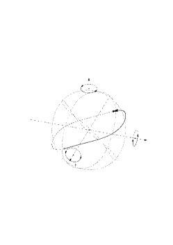
(a) Four bodies with dihedral symmetry and anti-symmetric constraint.

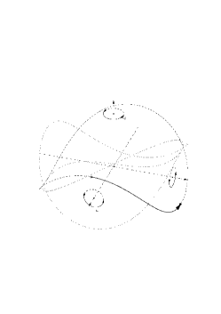
(b) Four bodies with dihedral symmetry and semi-coreography constraint.

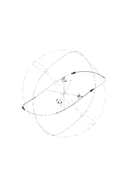
(c) Twelve bodies with dihedral symmetry and 3-coreography constraint.

Remark 4.9

Variational methods under symmetry constraints have been popular in the recent years, starting from Chenciner and Montgomery “figure eight” orbit [Che02, CM00]. Symmetric periodic minimisers have been found by many authors (to name a few, [ACZ94, Che02, Che03a, Che03b, SX05]). Periodic orbits dihedrally symmetric can be shown to exist as well: from [Fer06, Fer07, FT04] it follows that if $x(t)$ is a minimiser of the Lagrangean action functional, constrained to the Sobolev space of $G$-equivariant periodic trajectories (where $G$ is a cyclic extension of $D_{l}$), then $x(t)$ is collision-less. In the Figures 4(a), 4(b) and 4(c), some of the resulting orbits are shown, which are symmetric with respect to some cyclic extensions of the group $D_{l}$.

Appendix A Some pointwise estimates for the planar case

A.1 Proof of Proposition 3.4

The proof of this result will be divided into two main steps. The first correspond to the Newtonian case $\alpha=1$ and the second to the case $\alpha\in(0,1)$.

Moreover we refer to the right (left) unstable branch of $W^{u}({\bm{c}}_{-})$ as that having $u>0$ ($u<0$) in a small neighborhood of ${\bm{c}}_{-}$ in ${\mathscr{P}}$.

Using uniqueness of solutions, the symmetries and the gradient-like character of the flow with respect to $v$, it is sufficient to prove the following fact.

1. The right branch of $W^{u}({\bm{c}}_{-})$ intersects $\theta=\pi/2$ ($\theta=-\pi/2$, resp.) with $v<0$ and then intersects the section $v=0$ with an angle $\theta\in(0,\pi/4)$.

Proof in the Newtonian case.

The proof of this claim will be divided into some parts:

1. Upper bound for $v(\pi/2)$ in the case $u>0$ and $\theta\in(\pi/4,\pi/2)$.

   $$\dfrac{dv}{d\theta} =\sqrt{\dfrac{1}{4}\left[1+\dfrac{1}{\cos\theta}+\dfrac{1}{\sin\theta}\right]-\dfrac{v^{2}}{4}}\leq$$

   $$\leq\dfrac{1}{2}\sqrt{\dfrac{1}{\cos\theta}+{\bm{a}}_{2}}$$

   where

   $${\bm{a}}_{2}:=\max_{\theta\in[\pi/4,\pi/2]}f(\theta)=1+\sqrt{2},\qquad f(\theta)=1+\dfrac{1}{\sin\theta}.$$

   Thus

   $$v(\pi/2) \leq v(\pi/4)+\int_{\pi/4}^{\pi/2}\dfrac{1}{2}\sqrt{\dfrac{1}{\cos\theta}+{\bm{a}}_{2}}\ d\theta=_{\Phi:=\pi/2-\theta}$$

   $$=v(\pi/4)+\dfrac{1}{2}\int_{0}^{\pi/4}\sqrt{\dfrac{1}{\sin\Phi}+{\bm{a}}_{2}}\ d\Phi\leq$$

   $$\leq v(\pi/4)+\dfrac{1}{2}\int_{0}^{\pi/4}\sqrt{\dfrac{{\bm{a}}_{1}}{\Phi}+{\bm{a}}_{2}}\ d\Phi$$

   where ${\bm{a}}_{1}:=\max_{[0,\pi/4]}\dfrac{\Phi}{\sin\Phi}=\dfrac{\pi}{4}\sqrt{2}$ since the function $g(\Phi):=\dfrac{\Phi}{\sin\Phi}$ is increasing on $[0,\pi/4]$. Since $v(\pi/4)=-\sqrt{1+2\sqrt{2}}$ and by using the quadrature

   $$\int\sqrt{\dfrac{a}{x}+b}\,dx=\sqrt{x(a+bx)}+\dfrac{a}{2\sqrt{b}}\log[2\sqrt{b}\sqrt{(x(a+bx)}+2bx+a],$$

   it follows that

   $$v(\pi/2)\leq{\bm{v}}_{1}:=\dfrac{1}{2}\int_{0}^{\pi/4}\sqrt{\dfrac{\pi\sqrt{2}}{4\,x}+1+\sqrt{2}}-\sqrt{1+2\sqrt{2}}\approx{\bf-0.8014\/}<0,$$

   therefore $v$ intersects $\theta=\pi/2$ at a negative value.

2. Lower bound for $v(\pi/2)$ in the case $u>0$ and $\theta\in(\pi/4,\pi/2)$.
   Next we calculate a lower estimate for $v(\pi/2)$. For this we first observe that

   $$\dfrac{dv}{d\theta}=\dfrac{1}{2}\sqrt{1+\dfrac{1}{\sin\theta}+\dfrac{1}{\cos\theta}-v^{2}}\geq\dfrac{1}{2}\sqrt{\dfrac{1}{\cos\theta}+{\bm{a}}_{3}-v^{2}},$$

   where ${\bm{a}}_{3}:=\min_{\theta\in[\pi/4,\pi/2]}f(\theta)=2$. Now we consider the interval $J:=[3/8\pi,\pi/2]\subset[\pi/4,\pi/2]$ and by a direct calculation:

   $$\dfrac{dv}{d\theta}\geq\dfrac{1}{2}\sqrt{\dfrac{1}{\cos\theta}+2-v^{2}(\pi/4)}\ \Rightarrow v(\pi/2) \geq v(3/8\pi)+\dfrac{1}{2}\int_{3/8\pi}^{\pi/2}\sqrt{\dfrac{1}{\cos\theta}+2-v^{2}(\pi/4)}\ d\theta\geq$$

   $$\geq v(\pi/4)+\dfrac{1}{2}\int_{0}^{\pi/8}\sqrt{\dfrac{1}{\Phi}+{\bm{a}}_{4}}\ d\Phi$$

   $$\approx{\bf-1.4164}:={\bm{v}}_{2}<0,$$

   for $\Phi$ as above and ${\bm{a}}_{4}:=2-v^{2}(\pi/4)=1-2\sqrt{2}$; moreover in the last inequality we used the fact that $\sin\Phi\leq\Phi$. From (1a) &(1b) it follows that ${\bm{v}}_{2}\leq v(\theta)\leq{\bm{v}}_{1}$, for $\theta\in[\pi/4,\pi/2]$ and $u>0$.

3. The continuation of the right branch through double collision at $\theta=\pi/2$ for $u<0$. We affirm that $v$ remains negative in the interval $J$.

   In fact, for $u<0$

   $$-\dfrac{dv}{d\theta}\leq\dfrac{1}{2}\sqrt{\dfrac{1}{\cos\theta}+{\bm{a}}_{5}}$$

   for ${\bm{a}}_{5}:=f(3/8\pi)=1+2\,{\dfrac{1}{\sqrt{2+\sqrt{2}}}}\approx{2.0824}$ and$f$ as above. Let ${\bm{a}}_{6}:=g(\pi/8)=3/4\,{\dfrac{\pi}{\sqrt{2+\sqrt{2}}}}\approx{1.0260}$. Integrating we get:

   (39) $$v(3/8\pi) \leq v(\pi/2)+\dfrac{1}{2}\int_{3/8\pi}^{\pi/2}\sqrt{\dfrac{1}{\cos\theta}+{\bm{a}}_{5}}\ d\theta\leq$$

   $$\leq v(\pi/2)+\dfrac{1}{2}\int_{0}^{\pi/8}\sqrt{\dfrac{{\bm{a}}_{6}}{\Phi}+{\bm{a}}_{5}}\ d\Phi\leq{\bm{v}}_{1}+\dfrac{1}{2}\int_{0}^{\pi/8}\sqrt{\dfrac{{\bm{a}}_{6}}{\Phi}+{\bm{a}}_{5}}\ d\Phi$$

   $$\approx{\bm{v}}_{1}+{0.7111}\approx{\bf-0.0903}<0$$

   Therefore

   $${\bm{v}}_{2}\leq v(\pi/2)\leq v(\theta)\leq v(3/8\pi)<0,\qquad\textrm{for}\ \ \theta\in[3/8\pi,\pi/2],\ \ \textrm{and}\ \ u<0.$$

   Therefore

   $${\bm{v}}_{2}\leq v(\pi/2)\leq v(\theta)\leq v(3/8\pi)<0,\qquad\textrm{for}\ \ \theta\in[3/8\pi,\pi/2],\ \ \textrm{and}\ \ u<0.$$

4. The continuation of the right branch through double collision at $\theta=\pi/2$ for $u<0$. We affirm that $v$ remains negative at the point $\theta=\pi/4$.

   In fact, for $u<0$

   $$-\dfrac{dv}{d\theta}\leq\dfrac{1}{2}\sqrt{\dfrac{1}{\cos\theta}+{\bm{a}}_{5}}$$

   for ${\bm{a}}:=f(\pi/4)=1+2\sqrt{2}$ and$f$ as above. Let ${\bm{b}}:=g(\pi/4)=\pi/4\sqrt{2}$. Integrating we get:

   (40) $$v(\pi/4) \leq v(\pi/2)+\dfrac{1}{2}\int_{\pi/4}^{\pi/2}\sqrt{\dfrac{1}{\cos\theta}+{\bm{a}}}\ d\theta\leq$$

   $$\leq v(\pi/2)+\dfrac{1}{2}\int_{0}^{\pi/4}\sqrt{\dfrac{{\bm{b}}}{\Phi}+{\bm{a}}}\ d\Phi\leq{\bm{v}}_{1}+\dfrac{1}{2}\int_{0}^{\pi/4}\sqrt{\dfrac{{\bm{b}}}{\Phi}+{\bm{a}}}\ d\Phi$$

   $$\approx{\bm{v}}_{1}+{0.7445}={\bf-0.5630}<0$$

5. From the above inequality we get the estimates ${\bm{v}}_{2}^{2}\geq v(\theta)^{2}$, for all $\theta\in[3\pi/8,\pi/2]$ and $u<0$. Using this estimate we can write:

   $$-\dfrac{dv}{d\theta}=\dfrac{1}{2}\sqrt{1+\dfrac{1}{\sin\theta}+\dfrac{1}{\cos\theta}-v^{2}}\geq\dfrac{1}{2}\sqrt{\dfrac{1}{\cos\theta}+{\bm{a}}_{7}-{\bm{v}}_{2}^{2}}$$

   where ${\bm{a}}_{7}:=\min_{\theta\in[3/8\pi,\pi/2]}f(\theta)=f(\pi/2)=2$. By a direct integration we have:

   $$v(3/8\pi) \geq v(\pi/2)+\dfrac{1}{2}\int_{3/8\pi}^{\pi/2}\sqrt{\dfrac{1}{\cos\theta}+{\bm{a}}_{7}-{\bm{v}}_{2}^{2}}\ d\theta\geq$$

   $$\geq v(\pi/2)+\dfrac{1}{2}\int_{0}^{\pi/8}\sqrt{\dfrac{1}{\Phi}+2-{\bm{v}}_{2}^{2}}\ d\Phi$$

   $$\geq{\bm{v}}_{2}+\dfrac{1}{2}\int_{0}^{\pi/8}\sqrt{\dfrac{1}{\Phi}+2-{\bm{v}}_{2}^{2}}\ d\Phi\approx{\bf-0.7900}.$$

6. To finish the estimate for the continuation of the right branch through double collision, we now consider $\theta\in[0,3\pi/8]$ and $u<0$. We observe that in $\theta=\pi/4$, $U(\theta)$ has a relative minimum and therefore for $\theta\in[0,3\pi/8]$ we have $U(\theta)\geq U(\pi/4)$. Now let $\tilde{v}:=\sqrt{2U(\pi/4)}$; thus

   $$-\dfrac{dv}{d\theta}\geq\dfrac{1}{2}\sqrt{\tilde{v}^{2}-v^{2}}$$

   and by a direct integration, we have

   $$-\arcsin\left(\dfrac{v}{\tilde{v}}\right)\Big{|}_{v(0)}^{v(3\pi/8)}\geq\dfrac{1}{2}\int_{0}^{3\pi/8}d\theta=3\pi/16.$$

   Therefore

   $$v(0)\geq\tilde{v}\sin\left(3\pi/16+\arcsin(v(3\pi/8)/\tilde{v})\right)\geq\tilde{v}\sin\left(3\pi/16+\arcsin(-0.7900/\tilde{v})\right)\approx{\bf 0.3376}.$$

   We observe that this estimate could be refined by considering the interval $[0,\pi/4]$ instead of $[0,3\pi/8]$; however to do so we need an estimate from below for $v(\pi/4)$.

By symmetry, the same arguments holds also for the left branch of $W^{u}({\bm{c}}_{-})$. Now the thesis easily follows by the fact that the flow is of gradient-type with restpoints ${\bm{c}}_{-}$ and ${\bm{c}}_{+}$. $\Box\\$

Proof in the case $\alpha\in(0,1)$

Also in this case the proof of this claim will be divided into some parts:

1. Upper bound for $v(\pi/2)$ in the case $u>0$ and $\theta\in(\pi/4,\pi/2)$.

   $$\dfrac{dv}{d\theta} =\dfrac{1}{2}\sqrt{2^{1-\alpha}\left[1+\dfrac{1}{\cos^{\alpha}\theta}+\dfrac{1}{\sin^{\alpha}\theta}\right]-v^{2}}\leq\dfrac{1}{2^{1/2+\beta}}\sqrt{\left[1+\dfrac{1}{\cos^{\alpha}\theta}+\dfrac{1}{\sin^{\alpha}\theta}\right]}\leq$$

   $$\leq\dfrac{1}{2^{1/2+\beta}}\sqrt{\dfrac{1}{\cos^{\alpha}\theta}+{\bm{b}}_{2}}$$

   where

   $${\bm{b}}_{2}:=\max_{\theta\in[\pi/4,\pi/2]}h(\theta)=1+2^{\beta},\qquad h(\theta):=1+\dfrac{1}{\sin^{\alpha}\theta}.$$

   Thus

   $$v(\pi/2) \leq v(\pi/4)+\int_{\pi/4}^{\pi/2}\dfrac{1}{2^{1/2+\beta}}\sqrt{\dfrac{1}{\cos^{\alpha}\theta}+{\bm{b}}_{2}}\ d\theta=_{\Phi:=\pi/2-\theta}$$

   $$=v(\pi/4)+\dfrac{1}{2^{1/2+\beta}}\int_{0}^{\pi/4}\sqrt{\dfrac{1}{\sin^{\alpha}\Phi}+{\bm{b}}_{2}}\ d\Phi\leq$$

   $$\leq v(\pi/4)+\dfrac{1}{2^{1/2+\beta}}\int_{0}^{\pi/4}\sqrt{\dfrac{{\bm{b}}_{1}}{\Phi^{\alpha}}+{\bm{b}}_{2}}\ d\Phi\leq$$

   $$\leq-\dfrac{1}{2^{\beta-1/2}}\sqrt{1+2^{\beta+1}}+\dfrac{1}{2^{1/2+\beta}}\int_{0}^{\pi/4}\sqrt{\dfrac{{\bm{b}}_{1}}{\Phi^{2\beta}}+{\bm{b}}_{2}}\ d\Phi:={\bm{j}}_{1}(\beta),$$

   where ${\bm{b}}_{1}:=\max_{[0,\pi/4]}\left(\dfrac{\Phi}{\sin\Phi}\right)^{\alpha}=\left(\dfrac{\pi}{4}\sqrt{2}\right)^{\alpha}$ since $g(\Phi):=\left(\dfrac{\Phi}{\sin\Phi}\right)^{\alpha}$ is an increasing function. Since $(0,1/2)\ni\beta\mapsto{\bm{j}}_{1}(\beta)$ is an increasing function on the interval $(0,1/2)$, then we conclude that

   $$v(\pi/2)\leq{\bm{j}}_{1}(1/2)\approx{\bf-0.8013}:={\bm{w}}_{1}.$$

   Therefore $v$ intersects $\theta=\pi/2$ at a negative value.

2. Lower bound for $v(\pi/2)$ in the case $u>0$ and $\theta\in(\pi/4,\pi/2)$.

   Next we calculate a lower estimate for $v(\pi/2)$. For this we first observe that

   $$\dfrac{1}{2}\sqrt{2^{1-\alpha}\left[1+\dfrac{1}{\cos^{\alpha}\theta}+\dfrac{1}{\sin^{\alpha}\theta}\right]-v^{2}}\geq\dfrac{1}{2^{1/2+\beta}}\sqrt{\dfrac{1}{\cos^{\alpha}\theta}+{\bm{b}}_{3}-v^{2}},$$

   where ${\bm{b}}_{3}:=\min_{\theta\in[\pi/4,\pi/2]}h(\theta)=2$. Now we consider the interval $J:=[\pi/4,3\pi/8]$ and by a direct calculation, we have:

   $$\dfrac{dv}{d\theta} \geq\dfrac{1}{2^{1/2+\beta}}\sqrt{\dfrac{1}{\cos^{\alpha}\theta}+2-v^{2}(\pi/4)}\ \Rightarrow$$

   $$v(\pi/2) \geq v(3\pi/8)+\int_{3\pi/8}^{\pi/2}\dfrac{1}{2^{1/2+\beta}}\sqrt{\dfrac{1}{\cos^{\alpha}\theta}+2-v^{2}(\pi/4)}\ d\theta\geq$$

   $$\geq v(3\pi/8)+\int_{0}^{\pi/8}\dfrac{1}{2^{1/2+\beta}}\sqrt{\dfrac{1}{\Phi^{2\beta}}+1-2^{\beta+1}}\ d\Phi:={\bm{j}}_{2}(\beta).$$

   Since:

   $$v(3\pi/8):=v_{\beta}(3\pi/8)=-\sqrt{2^{1-2\beta}\left[1+\left(\dfrac{2\sqrt{2}}{1+\sqrt{2}}\right)^{\beta}+\left(\dfrac{2\sqrt{2}}{\sqrt{2}-1}\right)^{\beta}\right]};$$

   and since both the functions

   $$(0,1/2)\ni\beta\mapsto v_{\beta}(3\pi/8)\ \textrm{and}\ (0,1/2)\ni\beta\mapsto\int_{0}^{\pi/8}\dfrac{1}{2^{1/2+\beta}}\sqrt{\dfrac{1}{\Phi^{2\beta}}+1-2^{\beta+1}}$$

   are strictly increasing it immediately follows that also ${\bm{j}}_{2}$ is an increasing function and therefore we can conclude that

   $$v(\pi/2)\geq{\bm{j}}_{1}(1/2):={\bm{w}}_{2}\approx{\bf-1.6267}.$$

3. The continuation of the right branch through double collision at $\theta=\pi/2$ for $u<0$. We affirm that $v$ remains negative in the interval $J$.

   In fact, for $u<0$

   $$-\dfrac{dv}{d\theta}\leq\dfrac{1}{2}\sqrt{2^{1-\alpha}\left[\dfrac{1}{\cos^{\alpha}\theta}+{\bm{b}}_{5}\right]}$$

   for ${\bm{b}}_{5}:=h(3\pi/8)$ and $h$ as above. Let ${\bm{b}}_{6}:=g(\pi/8)$. Integrating we get:

   (41) $$v(3\pi/8) \leq v(\pi/2)+\dfrac{1}{2}\int_{3\pi/8}^{\pi/2}\dfrac{1}{2^{1/2+\beta}}\sqrt{\left[\dfrac{1}{\cos^{\alpha}\theta}+{\bm{b}}_{5}\right]}\ d\theta\leq$$

   $$\leq v(\pi/2)+\dfrac{1}{2}\int_{0}^{\pi/8}\dfrac{1}{2^{1/2+\beta}}\sqrt{\left[\dfrac{{\bm{b}}_{6}}{\Phi^{2\beta}}+{\bm{b}}_{5}\right]}\ d\Phi\leq$$

   $$\leq {\bm{w}}_{1}+\dfrac{1}{2}\int_{0}^{\pi/8}\dfrac{1}{2^{1/2+\beta}}\sqrt{\left[\dfrac{{\bm{b}}_{6}}{\Phi^{2\beta}}+{\bm{b}}_{5}\right]}\ d\Phi$$

   $$\approx{\bf-0.0902}.$$

   Therefore

   $${\bm{w}}_{2}\leq v(\pi/2)\leq v(\theta)\leq v(3\pi/8)<0,\qquad\textrm{for}\ \ \theta\in[3\pi/8,\pi/2],\ \ \textrm{and}\ \ u<0.$$

4. From the above inequality we get the estimates ${\bm{w}}_{2}^{2}\geq v(\theta)^{2}$, for all $\theta\in[3\pi/8,\pi/2]$ and $u<0$. Using this estimate we can write:

   $$-\dfrac{dv}{d\theta}=\dfrac{1}{2}\sqrt{2^{1-\alpha}\left[1+\dfrac{1}{\sin^{\alpha}\theta}+\dfrac{1}{\cos^{\alpha}\theta}\right]-v^{2}}\geq\dfrac{1}{2}\sqrt{2^{1-\alpha}\left[\dfrac{1}{\cos\theta}+{\bm{a}}_{7}\right]-{\bm{w}}_{2}^{2}}$$

   where ${\bm{a}}_{7}:=\min_{\theta\in[3\pi/8,\pi/2]}h(\theta)=h(\pi/2)=2$. By a direct integration we have:

   $$v(3\pi/8) \geq v(\pi/2)+\dfrac{1}{2}\int_{3\pi/8}^{\pi/2}\sqrt{2^{1-\alpha}\left[\dfrac{1}{\cos^{\alpha}\theta}+{\bm{a}}_{7}\right]-{\bm{w}}_{2}^{2}}\ d\theta\geq$$

   $$\geq v(\pi/2)+\dfrac{1}{2}\int_{0}^{\pi/8}\sqrt{2^{1-\alpha}\left[\dfrac{1}{\Phi^{\alpha}}+2\right]-{\bm{w}}_{2}^{2}}\ d\Phi\geq$$

   $$\geq{\bm{w}}_{2}+\dfrac{1}{2}\int_{0}^{\pi/8}\sqrt{2^{1-\alpha}\left[\dfrac{1}{\Phi^{\alpha}}+2\right]-{\bm{w}}_{2}^{2}}\ d\Phi\geq$$

   $$\geq {\bm{w}}_{2}+\dfrac{1}{2}\int_{0}^{\pi/8}\sqrt{\left[\dfrac{1}{\Phi}+2\right]-{\bm{w}}_{2}^{2}}\ d\Phi\approx{\bf-1.0276}.$$

5. The continuation of the right branch through double collision at $\theta=\pi/2$ for $u<0$. We affirm that $v$ remains negative at the point $\theta=\pi/4$.

   In fact, for $u<0$

   $$-\dfrac{dv}{d\theta}\leq\dfrac{1}{2}\sqrt{2^{1-\alpha}\left[\dfrac{1}{\cos^{\alpha}\theta}+{\bm{b}}_{5}\right]}$$

   for ${\bm{b}}_{5}:=h(\pi/4)$ and $h$ as above. Let ${\bm{b}}_{6}:=g(\pi/4)$. Integrating we get:

   (42) $$v(\pi/4) \leq v(\pi/2)+\dfrac{1}{2}\int_{\pi/4}^{\pi/2}\dfrac{1}{2^{1/2+\beta}}\sqrt{\left[\dfrac{1}{\cos^{\alpha}\theta}+{\bm{b}}_{5}\right]}\ d\theta\leq$$

   $$\leq v(\pi/2)+\dfrac{1}{2}\int_{0}^{\pi/4}\dfrac{1}{2^{1/2+\beta}}\sqrt{\left[\dfrac{{\bm{b}}_{6}}{\Phi^{2\beta}}+{\bm{b}}_{5}\right]}\ d\Phi\leq$$

   $$\leq {\bm{w}}_{1}+\dfrac{1}{2}\int_{0}^{\pi/4}\dfrac{1}{2^{1/2+\beta}}\sqrt{\left[\dfrac{{\bm{b}}_{6}}{\Phi^{2\beta}}+{\bm{b}}_{5}\right]}\ d\Phi$$

   $$\approx{\bf-0.2237}.$$

6. To finish the estimate for the continuation of the right branch through double collision, we now consider $\theta\in[0,\pi/8]$ and $u<0$. We observe that in $\theta=\pi/8$, $U(\theta)$ has a relative minimum and therefore for $\theta\in[0,\pi/8]$ we have $U(\theta)\geq U(\pi/8)$. Now let $\tilde{v}:=\sqrt{2U(\pi/8)}$; thus

   $$-\dfrac{dv}{d\theta}\geq\dfrac{1}{2}\sqrt{\tilde{v}^{2}-v^{2}}$$

   and by a direct integration, we have

   $$-\arcsin\left(\dfrac{v}{\tilde{v}}\right)\Big{|}^{v(\pi/8)}_{v(0)}\geq\dfrac{1}{2}\int_{0}^{\pi/8}d\theta=\pi/16.$$

   Therefore

   $$v(0)\geq\tilde{v}\sin\left(\pi/16+\arcsin\left(\dfrac{v(\pi/8)}{\tilde{v}}\right)\right)\geq\tilde{v}\sin\left(\pi/16+\arcsin\left(\dfrac{-0.3741}{\tilde{v}}\right)\right)\approx{\bf 0.3810}.$$

By symmetry, the same arguments holds also for the left branch of $W^{u}({\bm{c}}_{-})$. Now the thesis easily follows by the fact that the flow is of gradient-type with restpoints ${\bm{c}}_{-}$ and ${\bm{c}}_{+}$. $\Box\\$

A.2 Proof of Proposition 3.6

The proof of this result will be divided into several steps.

1. There exists $\alpha_{0}\in(1,2)$ such that for each $\alpha\in(1,\alpha_{0})$ the right branch of $W^{u}({\bm{c}}_{-})$ intersects $\theta=\pi/2$ ($\theta=-\pi/2$, resp.) with $v<0$ and then intersects the section $v=0$ with an angle $\theta\in(0,\pi/4)$.

2. There exists $\alpha_{1}\in(1,2)$ such that for each $\alpha\in(\alpha_{1},2)$ the right branch of $W^{u}({\bm{c}}_{-})$ intersects $\theta=\pi/2$ ($\theta=-\pi/2$, resp.) with $v<0$ and then intersects the section $v=0$ with an angle $\theta\in(\pi/4,\pi/2)$.

3. There exists $\alpha_{*}\in(\alpha_{0},\alpha_{1})$ such that the right branch of $W^{u}({\bm{c}}_{-})$ intersects the right branch of $W^{u}({\bm{c}}_{+})$.

In order to prove item 1 we shall proceed as in the proof of the previous proposition.

1. There exists $\alpha_{0}\in(1,2)$ such that for each $\alpha\in(1,\alpha_{0})$, $v(\pi/2)<0$.

• Upper bound for $v(\pi/2)$ in the case $u>0$ and $\theta\in(\pi/4,\pi/2)$.

  $$\dfrac{dv}{d\theta} =\dfrac{1}{2}\sqrt{2^{1-\alpha}\left[1+\dfrac{1}{\cos^{\alpha}\theta}+\dfrac{1}{\sin^{\alpha}\theta}\right]-v^{2}}\leq\dfrac{1}{2^{1/2+\beta}}\sqrt{\left[1+\dfrac{1}{\cos^{\alpha}\theta}+\dfrac{1}{\sin^{\alpha}\theta}\right]}\leq$$

  $$\leq\dfrac{1}{2^{1/2+\beta}}\sqrt{\dfrac{1}{\cos^{\alpha}\theta}+{\bm{b}}_{2}}$$

  where

  $${\bm{b}}_{2}:=\max_{\theta\in[\pi/4,\pi/2]}h(\theta)=1+2^{\beta},\qquad h(\theta):=1+\dfrac{1}{\sin^{\alpha}\theta}.$$

  Thus

  $$v(\pi/2) \leq v(\pi/4)+\int_{\pi/4}^{\pi/2}\dfrac{1}{2^{1/2+\beta}}\sqrt{\dfrac{1}{\cos^{\alpha}\theta}+{\bm{b}}_{2}}\ d\theta=_{\Phi:=\pi/2-\theta}$$

  $$=v(\pi/4)+\dfrac{1}{2^{1/2+\beta}}\int_{0}^{\pi/4}\sqrt{\dfrac{1}{\sin^{\alpha}\Phi}+{\bm{b}}_{2}}\ d\Phi\leq$$

  $$\leq v(\pi/4)+\dfrac{1}{2^{1/2+\beta}}\int_{0}^{\pi/4}\sqrt{\dfrac{{\bm{b}}_{1}}{\Phi^{\alpha}}+{\bm{b}}_{2}}\ d\Phi=$$

  $$=-\dfrac{1}{2^{\beta-1/2}}\sqrt{1+2^{\beta+1}}+\dfrac{1}{2^{1/2+\beta}}\int_{0}^{\pi/4}\sqrt{\dfrac{{\bm{b}}_{1}}{\Phi^{2\beta}}+{\bm{b}}_{2}}\ d\Phi:={\bm{k}}_{1}(\beta),$$

  where ${\bm{b}}_{1}:=\max_{[0,\pi/4]}\left(\dfrac{\Phi}{\sin\Phi}\right)^{\alpha}=\left(\dfrac{\pi}{4}\sqrt{2}\right)^{\alpha}$ since $g(\Phi):=\left(\dfrac{\Phi}{\sin\Phi}\right)^{\alpha}$ is an increasing function. We observe that $(1/2,1)\ni\beta\mapsto{\bm{k}}_{1}(\beta)$ is a continuous increasing function on the interval $(1/2,1)$. However it changes sign in the interval $A_{1}:=(1.4,1.6)$; in particular if $\alpha_{0}$ is any number in the open interval $(1,1.46136]$, then we can conclude that

  $$v(\pi/2)\leq{\bm{k}}_{1}(1/2)\approx{\bf-0.1659}:={\bm{w}}_{1}.$$

• Lower bound for $v(\pi/2)$ in the case $u>0$ and $\theta\in(\pi/4,\pi/2)$. For this we first observe that

  $$\dfrac{1}{2}\sqrt{2^{1-\alpha}\left[1+\dfrac{1}{\cos^{\alpha}\theta}+\dfrac{1}{\sin^{\alpha}\theta}\right]-v^{2}}\geq\dfrac{1}{2^{1/2+\beta}}\sqrt{\dfrac{1}{\cos^{\alpha}\theta}+{\bm{b}}_{3}-2^{\alpha-1}v^{2}},$$

  where ${\bm{b}}_{3}:=\min_{\theta\in[\pi/4,\pi/2]}h(\theta)=2$. Now we consider the interval $J:=[\pi/4,3\pi/8]$ and by a direct calculation, we have:

  $$\dfrac{dv}{d\theta} \geq\dfrac{1}{2^{1/2+\beta}}\sqrt{\dfrac{1}{\cos^{\alpha}\theta}+2-v^{2}(\pi/4)}\ \Rightarrow$$

  $$v(\pi/2) \geq v(3\pi/8)+\int_{3\pi/8}^{\pi/2}\dfrac{1}{2^{1/2+\beta}}\sqrt{\dfrac{1}{\cos^{\alpha}\theta}+2-v^{2}(\pi/4)}\ d\theta\geq$$

  $$\geq v(3\pi/8)+\int_{0}^{\pi/8}\dfrac{1}{2^{1/2+\beta}}\sqrt{\dfrac{1}{\Phi^{2\beta}}+1-2^{\beta+1}}\ d\Phi:={\bm{j}}_{2}(\beta).$$

  Since:

  $$v(3\pi/8):=v_{\beta}(3\pi/8)=-\sqrt{2^{1-2\beta}\left[1+\left(\dfrac{2\sqrt{2}}{1+\sqrt{2}}\right)^{\beta}+\left(\dfrac{2\sqrt{2}}{\sqrt{2}-1}\right)^{\beta}\right]};$$

  and since both the functions

  $$(0,1/2)\ni\beta\mapsto v_{\beta}(3\pi/8)\ \textrm{and}\ (0,1/2)\ni\beta\mapsto\int_{0}^{\pi/8}\dfrac{1}{2^{1/2+\beta}}\sqrt{\dfrac{1}{\Phi^{2\beta}}+1-2^{\beta+1}}$$

  are strictly increasing it immediately follows that also ${\bm{j}}_{2}$ is an increasing function and therefore we can conclude that

  $$v(\pi/2)\geq{\bm{j}}_{1}(1/2):={\bm{w}}_{2}\approx{\bf-1.6267}.$$

  We observe that for $\alpha\geq 1.1$ we have $v(\pi/2)\geq{\bm{j}}_{1}(0.55):={\bm{w}}_{3}\approx{\bf-1.5285}$ Therefore $v$ intersects $\theta=\pi/2$ at a negative value.

1. There exists $\alpha_{00}\in(1,\alpha_{0})$ such that the continuation of the right branch through double collision at $\theta=\pi/2$ for $u<0$, remains negative in the interval $[\pi/4,\pi/2]$.

In fact, for $u<0$

$$-\dfrac{dv}{d\theta}\leq\dfrac{1}{2}\sqrt{2^{1-\alpha}\left[\dfrac{1}{\cos^{\alpha}\theta}+{\bm{b}}_{5}\right]}$$

for ${\bm{b}}_{5}:=h(49\pi/100)$ and $h$ as above. Let ${\bm{b}}_{6}:=g(\pi/100)$. Integrating we get:

(43) $$v(49\pi/100) \leq v(\pi/2)+\dfrac{1}{2}\int_{49\pi/100}^{\pi/2}\dfrac{1}{2^{1/2+\beta}}\sqrt{\left[\dfrac{1}{\cos^{\alpha}\theta}+{\bm{b}}_{5}\right]}\ d\theta\leq$$

$$\leq v(\pi/2)+\dfrac{1}{2}\int_{0}^{\pi/100}\dfrac{1}{2^{1/2+\beta}}\sqrt{\left[\dfrac{{\bm{b}}_{6}}{\Phi^{2\beta}}+{\bm{b}}_{5}\right]}\ d\Phi\leq$$

$$\leq {\bm{w}}_{1}+\dfrac{1}{2}\int_{0}^{\pi/100}\dfrac{1}{2^{1/2+\beta}}\sqrt{\left[\dfrac{{\bm{b}}_{6}}{\Phi^{2\beta}}+{\bm{b}}_{5}\right]}\ d\Phi\leq$$

$$\leq-0.1659+\dfrac{1}{2}\int_{0}^{\pi/100}\dfrac{1}{2^{1/2+\beta}}\sqrt{\left[\dfrac{{\bm{b}}_{6}}{\Phi^{2\beta}}+{\bm{b}}_{5}\right]}\ d\Phi$$

$$\approx{\bf-0.0057},$$

which holds for $\alpha\in(1,1.1]$. Thus the thesis follows by choosing $\alpha_{00}=1.1$. Therefore

$${\bm{w}}_{2}\leq v(\pi/2)\leq v(\theta)\leq v(49\pi/100)<0,\qquad\textrm{for}\ \ \theta\in[49\pi/100,\pi/2],\ \ \textrm{and}\ \ u<0.$$

From the above inequality we get the estimates ${\bm{w}}_{2}^{2}\geq v(\theta)^{2}$, for all $\theta\in[49\pi/100,\pi/2]$ and $u<0$. Using this estimate we can write:

$$-\dfrac{dv}{d\theta}=\dfrac{1}{2}\sqrt{2^{1-\alpha}\left[1+\dfrac{1}{\sin^{\alpha}\theta}+\dfrac{1}{\cos^{\alpha}\theta}\right]-v^{2}}\geq\dfrac{1}{2}\sqrt{2^{1-\alpha}\left[\dfrac{1}{\cos\theta}+{\bm{a}}_{7}\right]-{\bm{w}}_{2}^{2}}$$

where ${\bm{a}}_{7}:=\min_{\theta\in[49\pi/100,\pi/2]}h(\theta)=h(\pi/2)=2$. By a direct integration we have:

$$v(49\pi/100) \geq v(\pi/2)+\dfrac{1}{2}\int_{49\pi/100}^{\pi/2}\sqrt{2^{1-\alpha}\left[\dfrac{1}{\cos^{\alpha}\theta}+{\bm{a}}_{7}\right]-{\bm{w}}_{2}^{2}}\ d\theta\geq$$

$$\geq v(\pi/2)+\dfrac{1}{2}\int_{0}^{\pi/100}\sqrt{2^{1-\alpha}\left[\dfrac{1}{\Phi^{\alpha}}+2\right]-{\bm{w}}_{2}^{2}}\ d\Phi\geq$$

$$\geq{\bm{w}}_{2}+\dfrac{1}{2}\int_{0}^{\pi/100}\sqrt{2^{1-\alpha}\left[\dfrac{1}{\Phi^{\alpha}}+2\right]-{\bm{w}}_{2}^{2}}\ d\Phi\geq$$

$$\geq{\bf-1.1804}.$$

• Now we prove that the continuation of the right branch through double collision is negative at the point $\theta=\pi/4$.

In fact, for $u<0$

$$-\dfrac{dv}{d\theta}\leq\dfrac{1}{2}\sqrt{2^{1-\alpha}\left[\dfrac{1}{\cos^{\alpha}\theta}+{\bm{b}}_{5}\right]}$$

for ${\bm{b}}_{5}:=h(\pi/4)$ and $h$ as above. Let ${\bm{b}}_{6}:=g(\pi/4)$. Integrating we get:

(44) $$v(\pi/4) \leq v(\pi/2)+\dfrac{1}{2}\int_{\pi/4}^{\pi/2}\dfrac{1}{2^{1/2+\beta}}\sqrt{\left[\dfrac{1}{\cos^{\alpha}\theta}+{\bm{b}}_{5}\right]}\ d\theta\leq$$

$$\leq v(\pi/2)+\dfrac{1}{2}\int_{0}^{\pi/4}\dfrac{1}{2^{1/2+\beta}}\sqrt{\left[\dfrac{{\bm{b}}_{6}}{\Phi^{2\beta}}+{\bm{b}}_{5}\right]}\ d\Phi\leq$$

$$\leq {\bm{w}}_{1}+\dfrac{1}{2}\int_{0}^{\pi/}\dfrac{1}{2^{1/2+\beta}}\sqrt{\left[\dfrac{{\bm{b}}_{6}}{\Phi^{2\beta}}+{\bm{b}}_{5}\right]}\ d\Phi\leq$$

$$\leq{\bm{k}}_{1}(\beta)+\dfrac{1}{2}\int_{0}^{\pi/4}\dfrac{1}{2^{1/2+\beta}}\sqrt{\left[\dfrac{{\bm{b}}_{6}}{\Phi^{2\beta}}+{\bm{b}}_{5}\right]}\ d\Phi\leq$$

$$\leq-0.6857+\dfrac{1}{2}\int_{0}^{\pi/4}\dfrac{1}{2^{1/2+\beta}}\sqrt{\left[\dfrac{{\bm{b}}_{6}}{\Phi^{2\beta}}+{\bm{b}}_{5}\right]}\ d\Phi\leq$$

$$\leq{\bf-0.0713}.$$

To finish the estimate for the continuation of the right branch through double collision, we now consider $\theta\in[0,\pi/8]$ and $u<0$. We observe that in $\theta=\pi/8$, $U(\theta)$ has a relative minimum and therefore for $\theta\in[0,\pi/8]$ we have $U(\theta)\geq U(\pi/8)$. Now let $\tilde{v}:=\sqrt{2U(\pi/8)}$; thus

$$-\dfrac{dv}{d\theta}\geq\dfrac{1}{2}\sqrt{\tilde{v}^{2}-v^{2}}$$

and by a direct integration, we have

$$-\arcsin\left(\dfrac{v}{\tilde{v}}\right)\Big{|}^{v(\pi/8)}_{v(0)}\geq\dfrac{1}{2}\int_{0}^{\pi/8}d\theta=\pi/16.$$

Therefore

$$v(0)\geq\tilde{v}\sin\left(\pi/16+\arcsin\left(\dfrac{v(\pi/8)}{\tilde{v}}\right)\right)\geq\tilde{v}\sin\left(\pi/16+\arcsin\left(\dfrac{-0.3741}{\tilde{v}}\right)\right)\approx{\bf 0.4948}.$$

By symmetry, the same arguments holds also for the left branch of $W^{u}({\bm{c}}_{-})$. Now the thesis easily follows by the fact that the flow is of gradient-type with restpoints ${\bm{c}}_{-}$ and ${\bm{c}}_{+}$.

1. There exists $\alpha_{01}\in(\alpha_{00},\alpha_{0})$ such that the continuation of the right branch through double collision at $\theta=\pi/2$ for $u<0$, changes sign in the interval $[\pi/4,\pi/2]$ for any $\alpha\in[\alpha_{01},\alpha_{0})$.

In fact, using this estimate we can write:

$$-\dfrac{dv}{d\theta}=\dfrac{1}{2}\sqrt{2^{1-\alpha}\left[1+\dfrac{1}{\sin^{\alpha}\theta}+\dfrac{1}{\cos^{\alpha}\theta}\right]-v^{2}}\geq\dfrac{1}{2}\sqrt{2^{1-\alpha}\left[\dfrac{1}{\cos\theta}+{\bm{a}}_{7}\right]-{\bm{w}}_{2}^{2}}$$

where ${\bm{a}}_{7}:=\min_{\theta\in[49\pi/100,\pi/2]}h(\theta)=h(\pi/2)=2$. By a direct integration we have:

$$v(49\pi/100) \geq v(\pi/2)+\dfrac{1}{2}\int_{49\pi/100}^{\pi/2}\sqrt{2^{1-\alpha}\left[\dfrac{1}{\cos^{\alpha}\theta}+{\bm{a}}_{7}\right]-{\bm{w}}_{2}^{2}}\ d\theta\geq$$

$$\geq v(\pi/2)+\dfrac{1}{2}\int_{0}^{\pi/100}\sqrt{2^{1-\alpha}\left[\dfrac{1}{\Phi^{\alpha}}+2\right]-{\bm{w}}_{2}^{2}}\ d\Phi\geq$$

$$\geq{\bm{w}}_{2}+\dfrac{1}{2}\int_{0}^{\pi/100}\sqrt{2^{1-\alpha}\left[\dfrac{1}{\Phi^{\alpha}}+2\right]-{\bm{w}}_{2}^{2}}\ d\Phi\geq$$

$$\geq{\bf-1.1804}.$$

To finish the estimate for the continuation of the right branch through double collision, we now consider $\theta\in[3\pi/8,\pi/2]$ and $u<0$. We observe that in $\theta=\pi/4$, $U(\theta)$ has a relative minimum and therefore for $\theta\in[\pi/4,49\pi/100]$ we have $U(\theta)\geq U(\pi/4)$. Now let $\tilde{v}:=\sqrt{2U(\pi/4)}$; thus

$$-\dfrac{dv}{d\theta}\geq\dfrac{1}{2}\sqrt{\tilde{v}^{2}-v^{2}}$$

and by a direct integration, we have

$$-\arcsin\left(\dfrac{v}{\tilde{v}}\right)\Big{|}^{v(49\pi/100)}_{v(\pi/4)}\geq\dfrac{1}{2}\int_{\pi/4}^{49\pi/100}d\theta=3\pi/25.$$

Therefore

$$v(\pi/4)\geq\tilde{v}\sin\left(3\pi/25+\arcsin\left(\dfrac{v(3\pi/25)}{\tilde{v}}\right)\right)\geq\tilde{v}\sin\left(3\pi/25+\arcsin\left(\dfrac{-1.1804}{\tilde{v}}\right)\right)\approx{\bf 0.0511}.$$

By symmetry, the same arguments holds also for the left branch of $W^{u}({\bm{c}}_{-})$. Now the thesis easily follows by the fact that the flow is of gradient-type with restpoints ${\bm{c}}_{-}$ and ${\bm{c}}_{+}$.

1. There exists $\alpha_{0*}\in(\alpha_{00},\alpha_{01})$ such that for the continuation of the right branch through double collision at $\theta=\pi/2$ for $u<0$, we have $v(\pi/4)=0$.

In order to prove this fact we consider the one parameter family of initial value problems:

(45) $$(P_{\alpha})\qquad\left\{\begin{array}[]{ll}\dfrac{dv}{d\theta}=\dfrac{1}{2}\sqrt{2^{1-\alpha}\left[1+\dfrac{1}{\cos^{\alpha}\theta}+\dfrac{1}{\sin^{\alpha}\theta}\right]-v^{2}}:={\bm{F}}_{\alpha}(\theta,v)\\ \\ v(\pi/4)=-\sqrt{2^{1-\alpha}(1+2^{\beta+1})},\end{array}\right.$$

which can be written in integral form as follows

$$v_{\alpha}(\theta)=v(\pi/4)+\int_{\pi/4}^{\theta}{\bm{F}}_{\alpha}(\bar{\theta},v(\bar{\theta}))\,d\bar{\theta},\qquad\forall\,\theta\in(\pi/4,\pi/2).$$

If $v$ is a classical ($\mathscr{C}^{1}$)-solution of the ivp above, then it is a $\mathscr{C}^{0}$-solution of the corresponding Volterra integral equation; moreover the function

$${\bm{I}}:[1,\alpha_{0})\longrightarrow\mathbb{R}:\alpha\longmapsto{\bm{I}}(\alpha):=\int_{\pi/4}^{\pi/2}{\bm{F}}_{\alpha}(\theta,v(\theta))\,d\theta,$$

is continuous, by taking into account the theorem on integrals depending on parameters. Thus the function

$${\bm{V}}:(1,\alpha_{0})\rightarrow\mathbb{R}:\alpha\mapsto{\bm{V}}(\alpha):=v_{\alpha}(\pi/2):=v(\pi/4)+{\bm{I}}(\alpha)$$

is continuous. Moreover by the monotonicity of the integral of a nonnegative function with respect to the domain of integration and by the fact that the map $\alpha\mapsto{\bm{F}}_{\alpha}(\theta,v)$ increases on $(1,2)$, it follows that the map ${\bm{V}}$ also increases. Furthermore ${\bm{V}}(\alpha_{00})<0$ and ${\bm{V}}(\alpha_{01})>0$; thus by taking into account the theorem of zeros of a continuous and increasing function, there exists a unique $\alpha_{*}$ in between such that $V(\alpha_{0*})=0$, which means nothing but that $v_{\alpha}(\pi/4)=0$.

In order to prove item 2, we proceed as follows.

1. There exists $\alpha_{1}\in(1,2)$ such that for each $\alpha\in(\alpha_{1},2)$, $v(\pi/2)>0$.

• Lower bound for $v(\pi/2)$ in the case $u>0$ and $\theta\in(\pi/4,\pi/2)$.

Next we calculate a lower estimate for $v(\pi/2)$. For this we first observe that

$$\dfrac{1}{2}\sqrt{2^{1-\alpha}\left[1+\dfrac{1}{\cos^{\alpha}\theta}+\dfrac{1}{\sin^{\alpha}\theta}\right]-v^{2}}\geq\dfrac{1}{2}\sqrt{2^{1-\alpha}\left[\dfrac{1}{\cos^{\alpha}\theta}+{\bm{b}}_{3}\right]-v^{2}},$$

where ${\bm{b}}_{3}:=\min_{\theta\in[\pi/4,\pi/2]}h(\theta)=2$. Now we consider the interval $J:=[3\pi/8,\pi/2]$ and by a direct calculation, we have:

$$\dfrac{dv}{d\theta} \geq\dfrac{1}{2}\sqrt{2^{1-\alpha}\left[\dfrac{1}{\cos^{\alpha}\theta}+2\right]-v^{2}(\pi/4)}\ \Rightarrow$$

$$v(\pi/2) \geq v(3\pi/8)+\int_{3\pi/8}^{\pi/2}\dfrac{1}{2^{1/2+\beta}}\sqrt{\dfrac{1}{\cos^{\alpha}\theta}+2-2^{\alpha-1}v^{2}(\pi/4)}\ d\theta\geq$$

$$\geq v(3\pi/8)+\int_{0}^{\pi/8}\dfrac{1}{2^{1/2+\beta}}\sqrt{\dfrac{1}{\Phi^{2\beta}}+1-2^{\beta+1}}\ d\Phi:={\bm{k}}_{2}(\beta).$$

We observe that:

$$v(3\pi/8):=v_{\beta}(3\pi/8)=-\sqrt{2^{1-2\beta}\left[1+\left(\dfrac{2\sqrt{2}}{1+\sqrt{2}}\right)^{\beta}+\left(\dfrac{2\sqrt{2}}{\sqrt{2}-1}\right)^{\beta}\right]}.$$

Moreover, the function below

$$(1/2,1)\ni\beta\mapsto v_{\beta}(3\pi/8)\ \textrm{and}\ (0,1/2)\ni\beta\mapsto\int_{0}^{\pi/8}\dfrac{1}{2^{1/2+\beta}}\sqrt{\dfrac{1}{\Phi^{2\beta}}+1-2^{\beta+1}}$$

as well as ${\bm{k}}_{2}$ are strictly increasing functions. However it changes sign and in particular it is positive in the interval $A_{2}:=[1.7,2)$. Therefore by choosing any number $\alpha_{1}\in A_{2}$ we can conclude that

$$v(\pi/2)\geq{\bm{k}}_{2}(1.7):={\bm{w}}_{2}\approx{\bf 0.1055}>0.$$

By symmetry, the same arguments holds also for the left branch of $W^{u}({\bm{c}}_{-})$. Now the thesis easily follows by the fact that the flow is of gradient-type with restpoints ${\bm{c}}_{-}$ and ${\bm{c}}_{+}$.

1. There exists a unique $\alpha_{*}\in(\alpha_{0},\alpha_{1})$ such that $v_{\alpha}(\pi/2)=0$.

In order to prove this fact we consider the one parameter family of initial value problems:

(46) $$(P_{\alpha})\qquad\left\{\begin{array}[]{ll}\dfrac{dv}{d\theta}=\dfrac{1}{2}\sqrt{2^{1-\alpha}\left[1+\dfrac{1}{\cos^{\alpha}\theta}+\dfrac{1}{\sin^{\alpha}\theta}\right]-v^{2}}:={\bm{F}}_{\alpha}(\theta,v)\\ \\ v(\pi/4)=-\sqrt{2^{1-\alpha}(1+2^{\beta+1})},\end{array}\right.$$

which can be written in integral form as follows

$$v_{\alpha}(\theta)=v(\pi/4)+\int_{\pi/4}^{\theta}{\bm{F}}_{\alpha}(\bar{\theta},v(\bar{\theta}))\,d\bar{\theta},\qquad\forall\,\theta\in(\pi/4,\pi/2).$$

If $v$ is a classical ($\mathscr{C}^{1}$)-solution of the ivp above, then it is a $\mathscr{C}^{0}$-solution of the corresponding Volterra integral equation; moreover the function

$${\bm{I}}:[1,2)\longrightarrow\mathbb{R}:\alpha\longmapsto{\bm{I}}(\alpha):=\int_{\pi/4}^{\pi/2}{\bm{F}}_{\alpha}(\theta,v(\theta))\,d\theta,$$

is continuous, by taking into account the theorem on integrals depending on parameters. Thus the function

$${\bm{V}}:(1,2)\rightarrow\mathbb{R}:\alpha\mapsto{\bm{V}}(\alpha):=v_{\alpha}(\pi/2):=v(\pi/4)+{\bm{I}}(\alpha)$$

is continuous. Moreover by the monotonicity of the integral of a nonnegative function with respect to the domain of integration and by the fact that the map $\alpha\mapsto{\bm{F}}_{\alpha}(\theta,v)$ increases on $(1,2)$, it follows that the map ${\bm{V}}$ also increases. Furthermore ${\bm{V}}(\alpha_{0})<0$ and ${\bm{V}}(\alpha_{1})>0$; thus by taking into account the theorem of zeros of a continuous and increasing function, there exists a unique $\alpha_{*}$ in between such that $V(\alpha_{*})=0$, which means nothing but that $v_{\alpha}(\pi/2)=0$. $\Box\\$

Appendix B Some pointwise estimates for the tetrahedral case

B.1 Proof of Proposition 3.7

The proof of this result will be divided into two main steps. The first correspond to the Newtonian case $\alpha=1$ and the second to the case $\alpha\in(0,1)$.

Moreover we refer to the right (left) unstable branch of $W^{u}({\bm{e}}^{-}_{11})$ as that having $u>0$ ($u<0$) in a small neighborhood of ${\bm{e}}^{-}_{11}$ in ${\mathscr{P}}$.

Using uniqueness of solutions, the symmetries and the gradient-like character of the flow with respect to $v$, it is sufficient to prove the following fact.

1. The right branch of $W^{u}({\bm{e}}^{-}_{11})$ intersects $\varphi=\pi/2$ ($\varphi=-\pi/2$, resp.) with $v<0$ and then intersects the section $v=0$ with an angle $\varphi>0$ (resp. $\varphi<0$).

Proof in the Newtonian case.

The proof of this claim will be divided into some parts:

1. Upper bound for $v(\pi/2)$ in the case $u>0$ and $\varphi\in(\varphi_{1},\pi/2)$, where $\varphi_{1}=\arctan(1/\sqrt{2})$.

   $$\dfrac{dv}{d\theta} =\dfrac{1}{2}\sqrt{\dfrac{1}{\cos\varphi}+\dfrac{2\sqrt{2}}{\sqrt{1+\sin^{2}\varphi}}-v^{2}}\leq$$

   $$\leq\dfrac{1}{2}\sqrt{\dfrac{1}{\cos\varphi}+{\bm{d}}_{1}}$$

   where

   $${\bm{d}}_{1}:=\max_{\varphi\in[\varphi_{1},\pi/2]}{\bm{m}}(\varphi)=\sqrt{6},\qquad{\bm{m}}(\varphi):=\dfrac{2\sqrt{2}}{\sqrt{1+\sin^{2}\varphi}}.$$

   We observe that the maximum is achieved at the point $\varphi_{1}$ since the function ${\bm{m}}$ is strictly decreasing on that interval; in fact

   $${\bm{m}}^{\prime}(\varphi)=-\dfrac{2\sqrt{2}\sin\varphi\cos\varphi}{(1+\sin^{2}\varphi)^{3/2}}.$$

   Thus

   $$v(\pi/2) \leq v(\varphi_{1})+\dfrac{1}{2}\int_{\varphi_{1}}^{\pi/2}\sqrt{\dfrac{1}{\cos\varphi}+{\bm{d}}_{1}}\ d\varphi=_{\Phi:=\pi/2-\varphi}$$

   $$=v(\varphi_{1})+\dfrac{1}{2}\int_{0}^{\pi/2-\varphi_{1}}\sqrt{\dfrac{1}{\sin\Phi}+{\bm{d}}_{1}}\ d\Phi\leq$$

   $$\leq v(\varphi_{1})+\dfrac{1}{2}\int_{0}^{\pi/2-\varphi_{1}}\sqrt{\dfrac{{\bm{d}}_{2}}{\Phi}+{\bm{d}}_{1}}\ d\Phi=\dfrac{1}{2}\left[-\sqrt{6\sqrt{6}}+\int_{0}^{\pi/2-\varphi_{1}}\sqrt{\dfrac{{\bm{d}}_{2}}{\Phi}+{\bm{d}}_{1}}\ d\Phi\right]$$

   where ${\bm{d}}_{2}:=\max_{[0,\pi/2-\varphi_{1}]}{\bm{n}}(\Phi)=\dfrac{\sqrt{6}}{2}\left(\dfrac{\pi}{2}-\arctan\dfrac{1}{\sqrt{2}}\right)$, since the function ${\bm{n}}(\Phi):=\dfrac{\Phi}{\sin\Phi}$ is increasing on $[0,\pi/2-\varphi_{1}]$. Since $v(\varphi_{1})=-\dfrac{\sqrt{6\sqrt{6}}}{2}$ and by using the quadrature

   $$\int\sqrt{\dfrac{a}{x}+b}\,dx=\sqrt{x(a+bx)}+\dfrac{a}{2\sqrt{b}}\log[2\sqrt{b}\sqrt{(x(a+bx)}+2bx+a],$$

   it follows that

   $$v(\pi/2)\leq{\bm{v}}_{1}:={\bf-0.5727\/}<0,$$

   therefore $v$ intersects $\theta=\pi/2$ at a negative value.

2. Lower bound for $v(\pi/2)$ in the case $u>0$ and $\varphi\in(\varphi_{1},\pi/2)$.
   Next we calculate a lower estimate for $v(\pi/2)$. For this we first observe that

   $$\dfrac{dv}{d\varphi}=\dfrac{1}{2}\sqrt{\dfrac{1}{\cos\varphi}+\dfrac{2\sqrt{2}}{\sqrt{1+\sin^{2}\varphi}}-v^{2}}\geq\dfrac{1}{2}\sqrt{\dfrac{1}{\cos\varphi}+{\bm{d}}_{3}-v^{2}},$$

   where ${\bm{d}}_{3}:=\min_{\phi\in[\varphi_{1}\,\pi/2]}{\bm{m}}(\varphi)=2$. Now we consider the interval $J:=[7/16\pi,\pi/2]\subset[\varphi_{1},\pi/2]$ and by a direct calculation:

   $$\dfrac{dv}{d\varphi}\geq\dfrac{1}{2}\sqrt{\dfrac{1}{\cos\varphi}+2-v^{2}(\varphi_{1})}\ \Rightarrow v(\pi/2) \geq v(7/16\pi)+\dfrac{1}{2}\int_{7/16\pi}^{\pi/2}\sqrt{\dfrac{1}{\cos\varphi}+2-v^{2}(\varphi_{1})}\ d\varphi\geq$$

   $$\geq v(\varphi_{1})+\dfrac{1}{2}\int_{0}^{\pi/16}\sqrt{\dfrac{1}{\Phi}+{\bm{d}}_{4}}\ d\Phi$$

   $$\geq{\bf-1.4994}:={\bm{v}}_{2}<0,$$

   for $\Phi$ as above and ${\bm{d}}_{4}:=2-v^{2}(\varphi_{1})=2-3\sqrt{6}/2$; moreover in the last inequality we used the fact that $\sin\Phi\leq\Phi$. From (1a) &(1b) it follows that ${\bm{v}}_{2}\leq v(\theta)\leq{\bm{v}}_{1}$, for $\varphi\in[\varphi_{1},\pi/2]$ and $u>0$.

3. The continuation of the right branch through double collision at $\theta=\pi/2$ for $u<0$. We affirm that $v$ remains negative in the interval $J$.

   In fact, for $u<0$

   $$-\dfrac{dv}{d\theta}\leq\dfrac{1}{2}\sqrt{\dfrac{1}{\cos\theta}+{\bm{d}}_{5}}$$

   for ${\bm{a}}_{5}:={\bm{m}}(7\pi/16)\approx{2.0193}$. Let ${\bm{d}}_{6}:={\bm{n}}(\pi/16)\approx{1.0064}$. Integrating we get:

   (47) $$v(3/8\pi) \leq v(\pi/2)+\dfrac{1}{2}\int_{7\pi/16}^{\pi/2}\sqrt{\dfrac{1}{\cos\varphi}+{\bm{d}}_{5}}\ d\varphi\leq$$

   $$\leq v(\pi/2)+\dfrac{1}{2}\int_{0}^{\pi/16}\sqrt{\dfrac{{\bm{d}}_{6}}{\Phi}+{\bm{d}}_{5}}\ d\Phi\leq{\bm{v}}_{1}+\dfrac{1}{2}\int_{0}^{\pi/16}\sqrt{\dfrac{{\bm{d}}_{6}}{\Phi}+{\bm{d}}_{5}}\ d\Phi$$

   $$\leq{\bm{v}}_{1}+{0.4723}\leq{\bf-0.1004}<0$$

   Therefore

   $${\bm{v}}_{2}\leq v(\pi/2)\leq v(\theta)\leq v(7\pi/16)<0,\qquad\textrm{for}\ \ \theta\in[7\pi/16,\pi/2],\ \ \textrm{and}\ \ u<0.$$

   Therefore

   $${\bm{v}}_{2}\leq v(\pi/2)\leq v(\theta)\leq v(7\pi/16)<0,\qquad\textrm{for}\ \ \theta\in[7\pi/16,\pi/2],\ \ \textrm{and}\ \ u<0.$$

4. From the above inequality we get the estimates ${\bm{v}}_{2}^{2}\geq v(\theta)^{2}$, for all $\theta\in[7\pi/16,\pi/2]$ and $u<0$. Using this estimate we can write:

   $$-\dfrac{dv}{d\varphi}=\dfrac{1}{2}\sqrt{2U(\varphi)-v^{2}}\geq\dfrac{1}{2}\sqrt{\dfrac{1}{\cos\varphi}+{\bm{d}}_{7}-{\bm{v}}_{2}^{2}}$$

   where ${\bm{a}}_{7}:=\min_{\varphi\in[7\pi/16,\pi/2]}{\bm{m}}(\varphi)=f(\pi/2)=2$. By a direct integration we have:

   $$v(7\pi/16) \geq v(\pi/2)+\dfrac{1}{2}\int_{7\pi/16}^{\pi/2}\sqrt{\dfrac{1}{\cos\varphi}+{\bm{d}}_{7}-{\bm{v}}_{2}^{2}}\ d\theta\geq$$

   $$\geq v(\pi/2)+\dfrac{1}{2}\int_{0}^{\pi/16}\sqrt{\dfrac{1}{\Phi}+2-{\bm{v}}_{2}^{2}}\ d\Phi$$

   $$\geq{\bm{v}}_{2}+\dfrac{1}{2}\int_{0}^{\pi/16}\sqrt{\dfrac{1}{\Phi}+{\bm{d}}_{8}}\ d\Phi\geq{\bm{v}}_{3}:={\bf-1.0600},$$

   where ${\bm{d}}_{8}:=2-{\bm{v}}_{2}^{2}$.

5. To finish the estimate for the continuation of the right branch through double collision, we now consider $\varphi\in[0,7\pi/16]$ and $u<0$. We observe that in $\varphi=\varphi_{1}$, $U(\theta)$ has a relative minimum and therefore for $\varphi\in[0,7\pi/16]$ we have $U(\varphi)\geq U(\varphi_{1})$. Now let $\tilde{v}:=\sqrt{2U(\varphi_{1})}$; thus

   $$-\dfrac{dv}{d\varphi}\geq\dfrac{1}{2}\sqrt{\bar{v}^{2}-v^{2}}$$

   and by a direct integration, we have

   $$-\arcsin\left(\dfrac{v}{\bar{v}}\right)\Big{|}_{v(0)}^{v(7\pi/16)}\geq\dfrac{1}{2}\int_{0}^{7\pi/16}d\theta=7\pi/32.$$

   Therefore

   $$v(0)\geq\tilde{v}\sin\left(7\pi/32+\arcsin(v(7\pi/16)/\bar{v})\right)\geq\bar{v}\sin\left(7\pi/32+\arcsin({\bm{v}}_{3}/\bar{v})\right)\geq{\bf 0.1937}.$$

By symmetry, the same arguments holds also for the left branch of $W^{u}({\bm{c}}_{-})$. Now the thesis easily follows by the fact that the flow is of gradient-type with restpoints ${\bm{c}}_{-}$ and ${\bm{c}}_{+}$.

1. The left branch of $W^{u}({\bm{e}}^{1}_{11})$ intersects $\varphi=-\pi/2$ with at a negative value of $v$.

In order to prove this claim we follow the idea used by [DV99].

Now we consider the left branch of $W^{u}({\bm{e}}^{-}_{11})$. It is clear that for the same value of $\varphi$, $v$ is greater along the left branch of $W^{u}({\bm{e}}^{-}_{11})$ that the corresponding value for the left branch of $W^{u}({\bm{e}}_{12}^{-})$, then due to the symmetries of the problem it follows that the left branch of $W^{u}({\bm{e}}_{11}^{-})$ meets the section $v=0$ for some value of $\varphi$ which is negative. It remains to prove that it actually meets $\varphi=-\pi/2$ at a negative value of $v$. For $u<0$, we have:

$$-\dfrac{dv}{d\varphi}=\sqrt{{\bm{a}}(\varphi)-\dfrac{v^{2}}{4}}$$

where ${\bm{a}}(\varphi):=\dfrac{U_{\mathrm{Tet}}(\varphi)}{2}=\dfrac{1}{4\cos\varphi}+\dfrac{\sqrt{2}}{2\sqrt{1+\sin^{2}\varphi}}$. If $I_{n}:=[\tilde{\varphi}_{n-1},\tilde{\varphi}_{n}]$ and ${\bm{a}}_{n}:=\max_{\varphi\in I_{n}}{\bm{a}}(\varphi)$, then for $\varphi\in I_{n}$, we have:

$$-\dfrac{dv}{d\varphi}\leq\sqrt{{\bm{a}}_{n}-\dfrac{v^{2}}{4}}.$$

By a direct integration, we can conclude that

(48) $$v(\tilde{\varphi}_{n})\leq 2\sqrt{{\bm{a}}_{n}}\sin\left(\dfrac{1}{2}|\tilde{\varphi}_{n}-\tilde{\varphi}_{n-1}|+\arcsin\left(\dfrac{v(\tilde{\varphi}_{n-1})}{2\sqrt{{\bm{a}}_{n}}}\right)\right).$$

It is readily verified that ${\bm{a}}_{n}=\dfrac{v(\tilde{\varphi}_{n})}{2}$ for any interval $I_{n}\subset[-\pi/2,-\varphi]\cup[0,\varphi_{1}]:={\bm{A}}$, since $\varphi\mapsto{\bm{a}}(\varphi)$ is positive and non-increasing on that subset; moreover ${\bm{a}}_{n}={\bm{a}}(\tilde{\varphi}_{n-1})$ in $[\pi/2,\pi/2]\setminus{\bm{A}}:={\bm{B}}$ since on this set this function is positive and non-decreasing. We define

$$\tilde{\varphi}_{n}=\dfrac{(12-n)\varphi_{1}}{12},\qquad\textrm{for each}\ \ n\,\in\,{\bf 36}.$$

Solving recursively the inequality, we obtain

$$v(\tilde{\varphi}_{32})=v(-5\varphi_{1}/3)\leq{\bf-1.1452.\/}$$

On the other side, for $\varphi\in[-\pi/2,5\varphi_{1}/3]$,

$$-\dfrac{dv}{d\varphi}\leq\dfrac{1}{2}\sqrt{\dfrac{1}{\cos\varphi}+{\bm{d}}_{9}}$$

where ${\bm{d}}_{9}:={\bm{m}}(-5\varphi_{1}/3)$. Again integrating and letting ${\bm{d}}_{10}:={\bm{n}}(\pi/2-5\varphi_{1}/3)$, we obtain:

(49) $$-v(5\varphi_{1}/3)+v(-\pi/2) \leq\dfrac{1}{2}\int_{-\pi/2}^{-5\varphi_{1}/3}\sqrt{\dfrac{1}{\cos\varphi}+{\bm{d}}_{9}}\,d\varphi$$

$$\leq\dfrac{1}{2}\int_{0}^{\pi/2-5\varphi_{1}/3}\sqrt{\dfrac{1}{\sin\Phi}+{\bm{d}}_{9}}\,d\Phi$$

$$\leq\dfrac{1}{2}\int_{0}^{\pi/2-5\varphi_{1}/3}\sqrt{\dfrac{{\bm{d}}_{10}}{\Phi}+{\bm{d}}_{9}}\,d\Phi$$

$$\leq{\bf 0.8803}$$

Now suppose that $v(-\pi/2)>0$; then from the inequality (49) it follows:

$$v(-5\varphi_{1}/3)\geq{\bf-0.8803}$$

which is a contradiction. We conclude that $v(-\pi/2)<0$ for the left branch of $W^{u}({\bm{e}}_{11}^{-})$.

$\Box\\$

Proof in the case $\alpha\in(0,1)$

The proof of this claim will be divided into some parts:

1. Upper bound for $v(\pi/2)$ in the case $u>0$ and $\varphi\in(\varphi_{1},\pi/2)$, where $\varphi_{1}=\arctan(1/\sqrt{2})$.

   $$\dfrac{dv}{d\theta} =\dfrac{1}{2}\sqrt{\dfrac{1}{(2\cos\varphi)^{\alpha}}+\dfrac{2^{1-\alpha/2}}{(1+\sin^{2}\varphi)^{\alpha/2}}-v^{2}}\leq\dfrac{1}{2}\sqrt{\dfrac{1}{(2\cos\varphi)^{\alpha}}+\dfrac{2^{1-\alpha/2}}{(1+\sin^{2}\varphi)^{\alpha/2}}}$$

   $$=\dfrac{1}{2^{1/2+\beta}}\sqrt{\dfrac{1}{\cos\varphi^{2\beta}}+\dfrac{2^{1+\beta}}{(1+\sin^{2}\varphi)^{\beta}}}\leq\dfrac{1}{2^{1/2+\beta}}\sqrt{\dfrac{1}{\cos\varphi^{2\beta}}+{\bm{e}}_{1}}$$

   where

   $${\bm{e}}_{1}:=\max_{\varphi\in[\varphi_{1},\pi/2]}{\bm{m}}(\beta,\varphi)=2^{1-\beta}3^{\beta}\qquad{\bm{m}}(\beta,\varphi):=\dfrac{2^{1+\beta}}{(1+\sin^{2}\varphi)^{\beta}}.$$

   In fact for each $\beta\in(0,1/2)$, the map $\varphi\mapsto m(\beta,\varphi)$ is strictly decreasing on the interval $[\varphi_{1},\pi/2]$; thus the maximum is achieved at the point $\varphi=\varphi_{1}$. Moreover

   $$\dfrac{\partial{\bm{m}}}{\partial\beta}=\dfrac{2^{1+\beta}}{(1+\sin^{2})^{\beta}}[\log 2-\log(1+\sin^{2}\varphi)]\qquad\dfrac{\partial{\bm{m}}}{\partial\varphi}=-\dfrac{2^{2+\beta}\beta\sin\varphi\cos\varphi}{(1+\sin^{2}\varphi)^{\beta+1}}$$

   Thus

   $$v(\pi/2) \leq v(\varphi_{1})+\dfrac{1}{2^{\beta+1/2}}\int_{\varphi_{1}}^{\pi/2}\sqrt{\dfrac{1}{\cos\varphi^{2\beta}}+{\bm{e}}_{1}}\ d\varphi=_{\Phi:=\pi/2-\varphi}$$

   $$=v(\varphi_{1})+\dfrac{1}{2^{\beta+1/2}}\int_{0}^{\pi/2-\varphi_{1}}\sqrt{\dfrac{1}{\sin\Phi^{2\beta}}+{\bm{e}}_{1}}\ d\Phi\leq$$

   $$\leq v(\varphi_{1})+\dfrac{1}{2^{\beta+1/2}}\int_{0}^{\pi/2-\varphi_{1}}\sqrt{\dfrac{{\bm{e}}_{2}}{\Phi^{2\beta}}+{\bm{e}}_{1}}\ d\Phi=$$

   $$=-\sqrt{6}\sqrt{3^{\beta}8^{-\beta}}+\dfrac{1}{2^{\beta+1/2}}\int_{0}^{\pi/2-\varphi_{1}}\sqrt{\dfrac{{\bm{e}}_{2}}{\Phi^{2\beta}}+{\bm{e}}_{1}}\ d\Phi:={\bm{j}}_{1}(\beta)$$

   where ${\bm{e}}_{2}:=\max_{[0,\pi/2-\varphi_{1}]}{\bm{n}}(\beta,\Phi)$ where ${\bm{n}}(\beta,\Phi)=\left(\dfrac{\Phi}{\sin\Phi}\right)^{2\beta}$. We observe that

   $$\dfrac{\partial{\bm{n}}}{\partial\beta}=2\left(\dfrac{\Phi}{\sin\Phi}\right)^{2\beta}\log\dfrac{\Phi}{\sin\Phi},\qquad\dfrac{\partial{\bm{n}}}{\partial\Phi}=\dfrac{2\beta\sin\Phi}{\Phi}\left[\left(\dfrac{\Phi}{\sin\Phi}\right)^{2\beta}\left(\dfrac{1}{\sin\Phi}-\dfrac{\Phi\cos\Phi}{\sin^{2}\Phi}\right)\right].$$

   Now since the function $[0,\pi/2-\varphi 1]\ni\Phi\mapsto{\bm{g}}(\Phi):=\dfrac{\Phi}{\sin\Phi}$ increases and its minimum is achieved at the point $\Phi=0$, then it follows that on that interval is greater than $1$. Therefore for each $\Phi\in[0,\pi/2-\varphi_{1}]$, $\beta\mapsto{\bm{n}}(\beta,\Phi)$ is an increasing function. By elementary consideration for each $\beta\in(0,1/2)$ the function $\Phi\mapsto{\bm{n}}(\beta,\Phi)$ is an increasing function. Therefore

   $${\bm{e}}_{2}:=\left[\dfrac{\sqrt{6}}{2}\left(\dfrac{\pi}{2}-\arctan\dfrac{1}{\sqrt{2}}\right)\right]^{2\beta}\leq\dfrac{\sqrt{6}}{2}\left(\dfrac{\pi}{2}-\arctan\dfrac{1}{\sqrt{2}}\right).$$

   Now, the function $(0,1/2)\ni\beta\mapsto{\bm{j}}_{1}(\beta)$ is a negative and increasing function. Therefore the supremum is at the point $\beta=1/2$. Thus by elementary calculations, it follows that

   $$v(\pi/2)\leq{\bm{v}}_{1}:={\bf-0.5727<0.\/}$$

   Therefore $v$ intersects $\varphi=\pi/2$ at a negative value.

2. Lower bound for $v(\pi/2)$ in the case $u>0$ and $\varphi\in(\varphi_{1},\pi/2)$.
   Next we calculate a lower estimate for $v(\pi/2)$. For this we first observe that

   $$\dfrac{dv}{d\varphi}=\dfrac{1}{2}\sqrt{\dfrac{2}{2^{2\beta}}\left[\dfrac{1}{\cos^{2\beta}\varphi}+\dfrac{2^{1+\beta}}{(1+\sin^{2}\varphi)^{\beta}}\right]-v^{2}}\geq\dfrac{1}{2}\sqrt{\dfrac{2}{2^{2\beta}}\left[\dfrac{1}{\cos^{2\beta}\varphi}+{\bm{e}}_{3}\right]-v^{2}},$$

   where ${\bm{e}}_{3}:=\min_{\varphi\in[\varphi_{1}\,\pi/2]}{\bm{m}}(\beta,\varphi)=2$. Now we consider the interval $J:=[7/16\pi,\pi/2]\subset[\varphi_{1},\pi/2]$ and by a direct calculation:

   $$\dfrac{dv}{d\varphi} \geq\dfrac{1}{2}\sqrt{\dfrac{2}{2^{2\beta}}\left[\dfrac{1}{\cos^{2\beta}(\varphi)}+2\right]-v^{2}(\varphi_{1})}\ \Rightarrow$$

   $$v(\pi/2)\geq v(7/16\pi)+\dfrac{1}{2}\int_{7/16\pi}^{\pi/2}\sqrt{\dfrac{2}{2^{2\beta}}\left[\dfrac{1}{\cos^{2\beta}\varphi}+2\right]-6\,3^{\beta}\,8^{-\beta}}\ d\varphi\geq$$

   $$\geq v(\varphi_{1})+\int_{0}^{\pi/16}\dfrac{1}{2^{\beta+1/2}}\sqrt{\dfrac{1}{\Phi^{2\beta}}+{\bm{e}}_{4}}\ d\Phi=-\sqrt{6\,3^{\beta}\,8^{-\beta}}+\int_{0}^{\pi/16}\dfrac{1}{2^{\beta+1/2}}\sqrt{\dfrac{1}{\Phi^{2\beta}}+{\bm{e}}_{4}}\ d\Phi,$$

   for ${\bm{e}}_{4}:=2-v^{2}(\varphi_{1})2^{2\beta}/2=2-3^{\beta+1}2^{-\beta}$; moreover in the last inequality we used the fact that $\sin\Phi\leq\Phi$. The function

   $${\bm{j}}_{2}(\beta):=\int_{0}^{\pi/16}\dfrac{1}{2^{\beta+1/2}}\sqrt{\dfrac{1}{\Phi^{2\beta}}+{\bm{e}}_{4}}$$

   is positive, increasing on the interval $[0,1/2]$; moreover ${\bm{j}}_{2}(0)=0$. Thus

   $$v(\pi/2)\geq-\sqrt{6\,3^{\beta}\,2^{-3\beta}}\geq{\bf-1.4993:={\bm{v}}_{2}\/}.$$

   From (1a) &(1b) it follows that ${\bm{v}}_{2}\leq v(\varphi)\leq{\bm{v}}_{1}$, for $\varphi\in[\varphi_{1},\pi/2]$ and $u>0$.

3. The continuation of the right branch through double collision at $\varphi=\pi/2$ for $u<0$. We affirm that $v$ remains negative in the interval $J$.

   In fact, for $u<0$

   $$-\dfrac{dv}{d\varphi}\leq\dfrac{1}{2}\sqrt{\dfrac{2}{2^{2\beta}}\left[\dfrac{1}{\cos^{2\beta}\varphi}+{\bm{e}}_{5}\right]}$$

   for ${\bm{e}}_{5}:={\bm{m}}(\beta,7\pi/16)$. Let ${\bm{d}}_{6}:={\bm{n}}(\beta,\pi/16)$. Integrating we get:

   (50) $$v(7/16\pi) \leq v(\pi/2)+\dfrac{1}{2^{\beta+1/2}}\int_{7\pi/16}^{\pi/2}\sqrt{\dfrac{1}{\cos^{2\beta}\varphi}+{\bm{e}}_{5}}\ d\varphi\leq$$

   $$\leq v(\pi/2)+\dfrac{1}{2^{\beta+1/2}}\int_{0}^{\pi/16}\sqrt{\dfrac{{\bm{e}}_{6}}{\Phi^{2\beta}}+{\bm{e}}_{5}}\ d\Phi\leq{\bm{v}}_{1}+\dfrac{1}{2^{\beta 1/2}}\int_{0}^{\pi/16}\sqrt{\dfrac{{\bm{e}}_{6}}{\Phi}+{\bm{e}}_{5}}\ d\Phi$$

   $$\leq-0.5727+\dfrac{1}{2^{\beta 1/2}}\int_{0}^{\pi/16}\sqrt{\dfrac{{\bm{e}}_{6}}{\Phi}+{\bm{e}}_{5}}\ d\Phi\leq{\bf-0.1004}<0$$

   Therefore

   $${\bm{v}}_{2}\leq v(\pi/2)\leq v(\theta)\leq v(7\pi/16)<0,\qquad\textrm{for}\ \ \theta\in[7\pi/16,\pi/2],\ \ \textrm{and}\ \ u<0.$$

   Therefore

   $${\bm{v}}_{2}\leq v(\pi/2)\leq v(\theta)\leq v(7\pi/16)<0,\qquad\textrm{for}\ \ \theta\in[7\pi/16,\pi/2],\ \ \textrm{and}\ \ u<0.$$

4. From the above inequality we get the estimates ${\bm{v}}_{2}^{2}\geq v(\theta)^{2}$, for all $\theta\in[7\pi/16,\pi/2]$ and $u<0$. Using this estimate we can write:

   $$-\dfrac{dv}{d\varphi} =\dfrac{1}{2}\sqrt{2U(\varphi)-v^{2}}=\dfrac{1}{2}\sqrt{\dfrac{2}{2^{2\beta}}\left[\dfrac{1}{\cos^{2\beta}\varphi}+\dfrac{2^{1+\beta}}{(1+\sin^{2}\varphi)^{\beta}}\right]-v^{2}}$$

   $$\geq\dfrac{1}{2}\sqrt{\dfrac{2}{2^{2\beta}}\left[\dfrac{1}{\cos^{2\beta}\varphi}+{\bm{e}}_{7}\right]-v^{2}}\geq\dfrac{1}{2}\sqrt{\dfrac{2}{2^{2\beta}}\left[\dfrac{1}{\cos^{2\beta}\varphi}+{\bm{e}}_{7}\right]-{\bm{v}}_{2}^{2}}$$

   where ${\bm{e}}_{7}:=\min_{\varphi\in[7\pi/16,\pi/2]}{\bm{m}}(\beta,\varphi)={\bm{m}}(\beta,\pi/2)=2$. By a direct integration we have:

   $$v(7\pi/16) \geq v(\pi/2)+\dfrac{1}{2}\int_{7\pi/16}^{\pi/2}\sqrt{\dfrac{2}{2^{2\beta}}\left[\dfrac{1}{\cos^{2\beta}\varphi}+2\right]-{\bm{v}}_{2}^{2}}\ d\varphi\geq$$

   $$\geq v(\pi/2)+\dfrac{1}{2}\int_{7\pi/16}^{\pi/2}\sqrt{\dfrac{2}{2^{2\beta}}\left[\dfrac{1}{\cos^{2\beta}\varphi}+2\right]-{\bm{v}}_{2}^{2}}\ d\varphi\geq$$

   $$\geq{\bm{v}}_{2}+\int_{7\pi/16}^{\pi/2}\dfrac{1}{2^{\beta+1/2}}\sqrt{\dfrac{1}{\cos^{2\beta}\varphi}+{\bm{e}}_{8}}\ d\varphi$$

   $$\geq{\bm{v}}_{2}+\int_{0}^{\pi/32}\dfrac{1}{2^{\beta+1/2}}\sqrt{\dfrac{1}{\sin^{2\beta}\Phi}+{\bm{e}}_{8}}\ d\Phi$$

   $$\geq{\bm{v}}_{2}+\int_{0}^{\pi/16}\dfrac{1}{2^{\beta+1/2}}\sqrt{\dfrac{1}{\Phi^{2\beta}}+{\bm{e}}_{8}}\ d\Phi\geq{\bm{v}}_{3}{\bf-1.2078}$$

   where ${\bm{e}}_{8}:=2-{\bm{v}}_{2}^{2}\,2^{2\beta-1}$.

5. To finish the estimate for the continuation of the right branch through double collision, we now consider $\varphi\in[0,7\pi/16]$ and $u<0$. We observe that in $\varphi=\varphi_{1}$, $U(\theta)$ has a relative minimum and therefore for $\varphi\in[0,7\pi/16]$ we have $U(\varphi)\geq U(\varphi_{1})$. Now let $\bar{v}:=\sqrt{2U(\varphi_{1})}$; thus

   $$-\dfrac{dv}{d\varphi}\geq\dfrac{1}{2}\sqrt{\bar{v}^{2}-v^{2}}$$

   and by a direct integration, we have

   $$-\arcsin\left(\dfrac{v}{\bar{v}}\right)\Big{|}_{v(0)}^{v(15\pi/32)}\geq\dfrac{1}{2}\int_{0}^{7\pi/16}d\theta=7\pi/32.$$

   Therefore

   $$v(0)\geq\bar{v}\sin\left(7\pi/32+\arcsin(v(7\pi/16)/\bar{v})\right)\geq\bar{v}\sin\left(7\pi/32+\arcsin({\bm{v}}_{2}/\bar{v})\right)\geq{\bf 0.4183}.$$

By symmetry, the same arguments holds also for the left branch of $W^{u}({\bm{c}}_{-})$. Now the thesis easily follows by the fact that the flow is of gradient-type with restpoints ${\bm{c}}_{-}$ and ${\bm{c}}_{+}$.

1. The left branch of $W^{u}({\bm{e}}^{1}_{11})$ intersects $\varphi=-\pi/2$ with at a negative value of $v$.

Now we consider the left branch of $W^{u}({\bm{e}}^{-}_{11})$. It is clear that for the same value of $\varphi$, $v$ is greater along the left branch of $W^{u}({\bm{e}}^{-}_{11})$ that the corresponding value for the left branch of $W^{u}({\bm{e}}_{12}^{-})$, then due to the symmetries of the problem it follows that the left branch of $W^{u}({\bm{e}}_{11}^{-})$ meets the section $v=0$ for some value of $\varphi$ which is negative. It remains to prove that it actually meets $\varphi=-\pi/2$ at a negative value of $v$. For $u<0$, we have:

$$-\dfrac{dv}{d\varphi}=\sqrt{{\bm{a}}(\beta,\varphi)-\dfrac{v^{2}}{4}}$$

where ${\bm{a}}(\beta,\varphi):=\dfrac{U_{\mathrm{Tet}}(\varphi)}{2}=\dfrac{1}{2^{1+2\beta}}\left[\dfrac{1}{\cos^{2\beta}\varphi}+\dfrac{2^{1+\beta}}{(1+\sin^{2}\varphi)^{\beta}}\right]$. If $I_{n}:=[\tilde{\varphi}_{n-1},\tilde{\varphi}_{n}]$ and ${\bm{a}}_{n}(\beta):=\max_{\varphi\in I_{n}}{\bm{a}}(\beta,\varphi)$, then for $\varphi\in I_{n}$, we have:

$$-\dfrac{dv}{d\varphi}\leq\sqrt{{\bm{a}}_{n}(\beta)-\dfrac{v^{2}}{4}}.$$

By a direct integration, we can conclude that

(51) $$v(\tilde{\varphi}_{n})\leq 2\sqrt{{\bm{a}}_{n}(\beta)}\sin\left(\dfrac{1}{2}|\tilde{\varphi}_{n}-\tilde{\varphi}_{n-1}|+\arcsin\left(\dfrac{v(\tilde{\varphi}_{n-1})}{2\sqrt{{\bm{a}}_{n}(\beta)}}\right)\right).$$

It is readily verified that ${\bm{a}}_{n}(\beta)=\dfrac{v(\tilde{\varphi}_{n})}{2}$ for any interval $I_{n}\subset[-\pi/2,-\varphi]\cup[0,\varphi_{1}]:={\bm{A}}$, since $\varphi\mapsto{\bm{a}}(\beta,\varphi)$ is positive and non-increasing on that subset; moreover ${\bm{a}}_{n}(\beta)={\bm{a}}(\beta,\tilde{\varphi}_{n-1})$ in $[\pi/2,\pi/2]\setminus{\bm{A}}:={\bm{B}}$ since on this set this function is positive and non-decreasing. We define

$$\varphi_{n}=\dfrac{(12-n)\varphi_{1}}{12},\qquad\textrm{for each}\ \ n\,\in\,{\bf 36}.$$

Solving recursively the inequality, we obtain

$$v(\varphi_{32})=v(-5\varphi_{1}/3)\leq{\bf-1.6699.\/}$$

On the other side, for $\varphi\in[-\pi/2,5\varphi_{1}/3]$,

$$-\dfrac{dv}{d\varphi}\leq\dfrac{1}{2^{\beta+1/2}}\sqrt{\dfrac{1}{\cos^{2\beta}\varphi}+{\bm{d}}_{9}}$$

where ${\bm{d}}_{9}:={\bm{m}}(\beta,-5\varphi_{1}/3)$. Again integrating (by setting $\Phi:=\pi/2+\varphi$) and letting ${\bm{d}}_{10}:={\bm{n}}(\beta,\pi/2-5\varphi_{1}/3)$, we obtain:

(52) $$-v(5\varphi_{1}/3)+v(-\pi/2) \leq\dfrac{1}{2^{\beta+1/2}}\int_{-\pi/2}^{-5\varphi_{1}/3}\sqrt{\dfrac{1}{\cos^{2\beta}\varphi}+{\bm{d}}_{9}}\,d\varphi$$

$$\leq\dfrac{1}{2^{\beta+1/2}}\int_{0}^{\pi/2-5\varphi_{1}/3}\sqrt{\dfrac{1}{\sin^{2\beta}\Phi}+{\bm{d}}_{9}}\,d\Phi$$

$$\leq\dfrac{1}{2^{\beta+1/2}}\int_{0}^{\pi/2-5\varphi_{1}/3}\sqrt{\dfrac{{\bm{d}}_{10}}{\Phi^{2\beta}}+{\bm{d}}_{9}}\,d\Phi$$

$$\leq{\bf 0.8721}.$$

Now suppose that $v(-\pi/2)>0$; then from the inequality (52) it follows:

$$v(-5\varphi_{1}/3)\geq{\bf-0.8721}$$

which is a contradiction. We conclude that $v(-\pi/2)<0$ for the left branch of $W^{u}({\bm{e}}_{11}^{-})$.

$\Box\\$

B.2 Proof of Proposition 3.9

The proof of this result will be divided into several steps.

1. There exists $\alpha_{0}\in(1,2)$ such that for each $\alpha\in(1,\alpha_{0})$ the right branch of $W^{u}({\bm{c}}_{-})$ intersects $\theta=\pi/2$ ($\theta=-\pi/2$, resp.) with $v<0$ and then intersects the section $v=0$ with an angle $\theta\in(0,\pi/4)$.

2. There exists $\alpha_{1}\in(1,2)$ such that for each $\alpha\in(\alpha_{1},2)$ the right branch of $W^{u}({\bm{c}}_{-})$ intersects $\theta=\pi/2$ ($\theta=-\pi/2$, resp.) with $v<0$ and then intersects the section $v=0$ with an angle $\theta\in(\pi/4,\pi/2)$.

3. There exists $\alpha_{*}\in(\alpha_{0},\alpha_{1})$ such that the right branch of $W^{u}({\bm{c}}_{-})$ intersects the right branch of $W^{u}({\bm{c}}_{+})$.

In order to prove item 1 we shall proceed as in the proof of the previous proposition.

1. There exists $\alpha_{0}\in(1,2)$ such that for each $\alpha\in(1,\alpha_{0})$, $v(\pi/2)<0$.

• Upper bound for $v(\pi/2)$ in the case $u>0$ and $\theta\in(\pi/4,\pi/2)$.

  $$\dfrac{dv}{d\theta} =\dfrac{1}{2}\sqrt{2^{1-\alpha}\left[1+\dfrac{1}{\cos^{\alpha}\theta}+\dfrac{1}{\sin^{\alpha}\theta}\right]-v^{2}}\leq\dfrac{1}{2^{1/2+\beta}}\sqrt{\left[1+\dfrac{1}{\cos^{\alpha}\theta}+\dfrac{1}{\sin^{\alpha}\theta}\right]}\leq$$

  $$\leq\dfrac{1}{2^{1/2+\beta}}\sqrt{\dfrac{1}{\cos^{\alpha}\theta}+{\bm{b}}_{2}}$$

  where

  $${\bm{b}}_{2}:=\max_{\theta\in[\pi/4,\pi/2]}h(\theta)=1+2^{\beta},\qquad h(\theta):=1+\dfrac{1}{\sin^{\alpha}\theta}.$$

  Thus

  $$v(\pi/2) \leq v(\pi/4)+\int_{\pi/4}^{\pi/2}\dfrac{1}{2^{1/2+\beta}}\sqrt{\dfrac{1}{\cos^{\alpha}\theta}+{\bm{b}}_{2}}\ d\theta=_{\Phi:=\pi/2-\theta}$$

  $$=v(\pi/4)+\dfrac{1}{2^{1/2+\beta}}\int_{0}^{\pi/4}\sqrt{\dfrac{1}{\sin^{\alpha}\Phi}+{\bm{b}}_{2}}\ d\Phi\leq$$

  $$\leq v(\pi/4)+\dfrac{1}{2^{1/2+\beta}}\int_{0}^{\pi/4}\sqrt{\dfrac{{\bm{b}}_{1}}{\Phi^{\alpha}}+{\bm{b}}_{2}}\ d\Phi=$$

  $$=-\dfrac{1}{2^{\beta-1/2}}\sqrt{1+2^{\beta+1}}+\dfrac{1}{2^{1/2+\beta}}\int_{0}^{\pi/4}\sqrt{\dfrac{{\bm{b}}_{1}}{\Phi^{2\beta}}+{\bm{b}}_{2}}\ d\Phi:={\bm{k}}_{1}(\beta),$$

  where ${\bm{b}}_{1}:=\max_{[0,\pi/4]}\left(\dfrac{\Phi}{\sin\Phi}\right)^{\alpha}=\left(\dfrac{\pi}{4}\sqrt{2}\right)^{\alpha}$ since $g(\Phi):=\left(\dfrac{\Phi}{\sin\Phi}\right)^{\alpha}$ is an increasing function. We observe that $(1/2,1)\ni\beta\mapsto{\bm{k}}_{1}(\beta)$ is a continuous increasing function on the interval $(1/2,1)$. However it changes sign in the interval $A_{1}:=(1.4,1.6)$; in particular if $\alpha_{0}$ is any number in the open interval $(1,1.46136]$, then we can conclude that

  $$v(\pi/2)\leq{\bm{k}}_{1}(1/2)\approx{\bf-0.1659}:={\bm{w}}_{1}.$$

• Lower bound for $v(\pi/2)$ in the case $u>0$ and $\theta\in(\pi/4,\pi/2)$. For this we first observe that

  $$\dfrac{1}{2}\sqrt{2^{1-\alpha}\left[1+\dfrac{1}{\cos^{\alpha}\theta}+\dfrac{1}{\sin^{\alpha}\theta}\right]-v^{2}}\geq\dfrac{1}{2^{1/2+\beta}}\sqrt{\dfrac{1}{\cos^{\alpha}\theta}+{\bm{b}}_{3}-2^{\alpha-1}v^{2}},$$

  where ${\bm{b}}_{3}:=\min_{\theta\in[\pi/4,\pi/2]}h(\theta)=2$. Now we consider the interval $J:=[\pi/4,3\pi/8]$ and by a direct calculation, we have:

  $$\dfrac{dv}{d\theta} \geq\dfrac{1}{2^{1/2+\beta}}\sqrt{\dfrac{1}{\cos^{\alpha}\theta}+2-v^{2}(\pi/4)}\ \Rightarrow$$

  $$v(\pi/2) \geq v(3\pi/8)+\int_{3\pi/8}^{\pi/2}\dfrac{1}{2^{1/2+\beta}}\sqrt{\dfrac{1}{\cos^{\alpha}\theta}+2-v^{2}(\pi/4)}\ d\theta\geq$$

  $$\geq v(3\pi/8)+\int_{0}^{\pi/8}\dfrac{1}{2^{1/2+\beta}}\sqrt{\dfrac{1}{\Phi^{2\beta}}+1-2^{\beta+1}}\ d\Phi:={\bm{j}}_{2}(\beta).$$

  Since:

  $$v(3\pi/8):=v_{\beta}(3\pi/8)=-\sqrt{2^{1-2\beta}\left[1+\left(\dfrac{2\sqrt{2}}{1+\sqrt{2}}\right)^{\beta}+\left(\dfrac{2\sqrt{2}}{\sqrt{2}-1}\right)^{\beta}\right]};$$

  and since both the functions

  $$(0,1/2)\ni\beta\mapsto v_{\beta}(3\pi/8)\ \textrm{and}\ (0,1/2)\ni\beta\mapsto\int_{0}^{\pi/8}\dfrac{1}{2^{1/2+\beta}}\sqrt{\dfrac{1}{\Phi^{2\beta}}+1-2^{\beta+1}}$$

  are strictly increasing it immediately follows that also ${\bm{j}}_{2}$ is an increasing function and therefore we can conclude that

  $$v(\pi/2)\geq{\bm{j}}_{1}(1/2):={\bm{w}}_{2}\approx{\bf-1.6267}.$$

  We observe that for $\alpha\geq 1.1$ we have $v(\pi/2)\geq{\bm{j}}_{1}(0.55):={\bm{w}}_{3}\approx{\bf-1.5285}$ Therefore $v$ intersects $\theta=\pi/2$ at a negative value.

1. There exists $\alpha_{00}\in(1,\alpha_{0})$ such that the continuation of the right branch through double collision at $\theta=\pi/2$ for $u<0$, remains negative in the interval $[\pi/4,\pi/2]$.

In fact, for $u<0$

$$-\dfrac{dv}{d\theta}\leq\dfrac{1}{2}\sqrt{2^{1-\alpha}\left[\dfrac{1}{\cos^{\alpha}\theta}+{\bm{b}}_{5}\right]}$$

for ${\bm{b}}_{5}:=h(49\pi/100)$ and $h$ as above. Let ${\bm{b}}_{6}:=g(\pi/100)$. Integrating we get:

(53) $$v(49\pi/100) \leq v(\pi/2)+\dfrac{1}{2}\int_{49\pi/100}^{\pi/2}\dfrac{1}{2^{1/2+\beta}}\sqrt{\left[\dfrac{1}{\cos^{\alpha}\theta}+{\bm{b}}_{5}\right]}\ d\theta\leq$$

$$\leq v(\pi/2)+\dfrac{1}{2}\int_{0}^{\pi/100}\dfrac{1}{2^{1/2+\beta}}\sqrt{\left[\dfrac{{\bm{b}}_{6}}{\Phi^{2\beta}}+{\bm{b}}_{5}\right]}\ d\Phi\leq$$

$$\leq {\bm{w}}_{1}+\dfrac{1}{2}\int_{0}^{\pi/100}\dfrac{1}{2^{1/2+\beta}}\sqrt{\left[\dfrac{{\bm{b}}_{6}}{\Phi^{2\beta}}+{\bm{b}}_{5}\right]}\ d\Phi\leq$$

$$\leq-0.1659+\dfrac{1}{2}\int_{0}^{\pi/100}\dfrac{1}{2^{1/2+\beta}}\sqrt{\left[\dfrac{{\bm{b}}_{6}}{\Phi^{2\beta}}+{\bm{b}}_{5}\right]}\ d\Phi$$

$$\approx{\bf-0.0057},$$

which holds for $\alpha\in(1,1.1]$. Thus the thesis follows by choosing $\alpha_{00}=1.1$. Therefore

$${\bm{w}}_{2}\leq v(\pi/2)\leq v(\theta)\leq v(49\pi/100)<0,\qquad\textrm{for}\ \ \theta\in[49\pi/100,\pi/2],\ \ \textrm{and}\ \ u<0.$$

From the above inequality we get the estimates ${\bm{w}}_{2}^{2}\geq v(\theta)^{2}$, for all $\theta\in[49\pi/100,\pi/2]$ and $u<0$. Using this estimate we can write:

$$-\dfrac{dv}{d\theta}=\dfrac{1}{2}\sqrt{2^{1-\alpha}\left[1+\dfrac{1}{\sin^{\alpha}\theta}+\dfrac{1}{\cos^{\alpha}\theta}\right]-v^{2}}\geq\dfrac{1}{2}\sqrt{2^{1-\alpha}\left[\dfrac{1}{\cos\theta}+{\bm{a}}_{7}\right]-{\bm{w}}_{2}^{2}}$$

where ${\bm{a}}_{7}:=\min_{\theta\in[49\pi/100,\pi/2]}h(\theta)=h(\pi/2)=2$. By a direct integration we have:

$$v(49\pi/100) \geq v(\pi/2)+\dfrac{1}{2}\int_{49\pi/100}^{\pi/2}\sqrt{2^{1-\alpha}\left[\dfrac{1}{\cos^{\alpha}\theta}+{\bm{a}}_{7}\right]-{\bm{w}}_{2}^{2}}\ d\theta\geq$$

$$\geq v(\pi/2)+\dfrac{1}{2}\int_{0}^{\pi/100}\sqrt{2^{1-\alpha}\left[\dfrac{1}{\Phi^{\alpha}}+2\right]-{\bm{w}}_{2}^{2}}\ d\Phi\geq$$

$$\geq{\bm{w}}_{2}+\dfrac{1}{2}\int_{0}^{\pi/100}\sqrt{2^{1-\alpha}\left[\dfrac{1}{\Phi^{\alpha}}+2\right]-{\bm{w}}_{2}^{2}}\ d\Phi\geq$$

$$\geq{\bf-1.1804}.$$

• Now we prove that the continuation of the right branch through double collision is negative at the point $\theta=\pi/4$.

In fact, for $u<0$

$$-\dfrac{dv}{d\theta}\leq\dfrac{1}{2}\sqrt{2^{1-\alpha}\left[\dfrac{1}{\cos^{\alpha}\theta}+{\bm{b}}_{5}\right]}$$

for ${\bm{b}}_{5}:=h(\pi/4)$ and $h$ as above. Let ${\bm{b}}_{6}:=g(\pi/4)$. Integrating we get:

(54) $$v(\pi/4) \leq v(\pi/2)+\dfrac{1}{2}\int_{\pi/4}^{\pi/2}\dfrac{1}{2^{1/2+\beta}}\sqrt{\left[\dfrac{1}{\cos^{\alpha}\theta}+{\bm{b}}_{5}\right]}\ d\theta\leq$$

$$\leq v(\pi/2)+\dfrac{1}{2}\int_{0}^{\pi/4}\dfrac{1}{2^{1/2+\beta}}\sqrt{\left[\dfrac{{\bm{b}}_{6}}{\Phi^{2\beta}}+{\bm{b}}_{5}\right]}\ d\Phi\leq$$

$$\leq {\bm{w}}_{1}+\dfrac{1}{2}\int_{0}^{\pi/}\dfrac{1}{2^{1/2+\beta}}\sqrt{\left[\dfrac{{\bm{b}}_{6}}{\Phi^{2\beta}}+{\bm{b}}_{5}\right]}\ d\Phi\leq$$

$$\leq{\bm{k}}_{1}(\beta)+\dfrac{1}{2}\int_{0}^{\pi/4}\dfrac{1}{2^{1/2+\beta}}\sqrt{\left[\dfrac{{\bm{b}}_{6}}{\Phi^{2\beta}}+{\bm{b}}_{5}\right]}\ d\Phi\leq$$

$$\leq-0.6857+\dfrac{1}{2}\int_{0}^{\pi/4}\dfrac{1}{2^{1/2+\beta}}\sqrt{\left[\dfrac{{\bm{b}}_{6}}{\Phi^{2\beta}}+{\bm{b}}_{5}\right]}\ d\Phi\leq$$

$$\leq{\bf-0.0713}.$$

To finish the estimate for the continuation of the right branch through double collision, we now consider $\theta\in[0,\pi/8]$ and $u<0$. We observe that in $\theta=\pi/8$, $U(\theta)$ has a relative minimum and therefore for $\theta\in[0,\pi/8]$ we have $U(\theta)\geq U(\pi/8)$. Now let $\tilde{v}:=\sqrt{2U(\pi/8)}$; thus

$$-\dfrac{dv}{d\theta}\geq\dfrac{1}{2}\sqrt{\tilde{v}^{2}-v^{2}}$$

and by a direct integration, we have

$$-\arcsin\left(\dfrac{v}{\tilde{v}}\right)\Big{|}^{v(\pi/8)}_{v(0)}\geq\dfrac{1}{2}\int_{0}^{\pi/8}d\theta=\pi/16.$$

Therefore

$$v(0)\geq\tilde{v}\sin\left(\pi/16+\arcsin\left(\dfrac{v(\pi/8)}{\tilde{v}}\right)\right)\geq\tilde{v}\sin\left(\pi/16+\arcsin\left(\dfrac{-0.3741}{\tilde{v}}\right)\right)\approx{\bf 0.4948}.$$

By symmetry, the same arguments holds also for the left branch of $W^{u}({\bm{c}}_{-})$. Now the thesis easily follows by the fact that the flow is of gradient-type with restpoints ${\bm{c}}_{-}$ and ${\bm{c}}_{+}$.

1. There exists $\alpha_{01}\in(\alpha_{00},\alpha_{0})$ such that the continuation of the right branch through double collision at $\theta=\pi/2$ for $u<0$, changes sign in the interval $[\pi/4,\pi/2]$ for any $\alpha\in[\alpha_{01},\alpha_{0})$.

In fact, using this estimate we can write:

$$-\dfrac{dv}{d\theta}=\dfrac{1}{2}\sqrt{2^{1-\alpha}\left[1+\dfrac{1}{\sin^{\alpha}\theta}+\dfrac{1}{\cos^{\alpha}\theta}\right]-v^{2}}\geq\dfrac{1}{2}\sqrt{2^{1-\alpha}\left[\dfrac{1}{\cos\theta}+{\bm{a}}_{7}\right]-{\bm{w}}_{2}^{2}}$$

where ${\bm{a}}_{7}:=\min_{\theta\in[49\pi/100,\pi/2]}h(\theta)=h(\pi/2)=2$. By a direct integration we have:

$$v(49\pi/100) \geq v(\pi/2)+\dfrac{1}{2}\int_{49\pi/100}^{\pi/2}\sqrt{2^{1-\alpha}\left[\dfrac{1}{\cos^{\alpha}\theta}+{\bm{a}}_{7}\right]-{\bm{w}}_{2}^{2}}\ d\theta\geq$$

$$\geq v(\pi/2)+\dfrac{1}{2}\int_{0}^{\pi/100}\sqrt{2^{1-\alpha}\left[\dfrac{1}{\Phi^{\alpha}}+2\right]-{\bm{w}}_{2}^{2}}\ d\Phi\geq$$

$$\geq{\bm{w}}_{2}+\dfrac{1}{2}\int_{0}^{\pi/100}\sqrt{2^{1-\alpha}\left[\dfrac{1}{\Phi^{\alpha}}+2\right]-{\bm{w}}_{2}^{2}}\ d\Phi\geq$$

$$\geq{\bf-1.1804}.$$

To finish the estimate for the continuation of the right branch through double collision, we now consider $\theta\in[3\pi/8,\pi/2]$ and $u<0$. We observe that in $\theta=\pi/4$, $U(\theta)$ has a relative minimum and therefore for $\theta\in[\pi/4,49\pi/100]$ we have $U(\theta)\geq U(\pi/4)$. Now let $\tilde{v}:=\sqrt{2U(\pi/4)}$; thus

$$-\dfrac{dv}{d\theta}\geq\dfrac{1}{2}\sqrt{\tilde{v}^{2}-v^{2}}$$

and by a direct integration, we have

$$-\arcsin\left(\dfrac{v}{\tilde{v}}\right)\Big{|}^{v(49\pi/100)}_{v(\pi/4)}\geq\dfrac{1}{2}\int_{\pi/4}^{49\pi/100}d\theta=3\pi/25.$$

Therefore

$$v(\pi/4)\geq\tilde{v}\sin\left(3\pi/25+\arcsin\left(\dfrac{v(3\pi/25)}{\tilde{v}}\right)\right)\geq\tilde{v}\sin\left(3\pi/25+\arcsin\left(\dfrac{-1.1804}{\tilde{v}}\right)\right)\approx{\bf 0.0511}.$$

By symmetry, the same arguments holds also for the left branch of $W^{u}({\bm{c}}_{-})$. Now the thesis easily follows by the fact that the flow is of gradient-type with restpoints ${\bm{c}}_{-}$ and ${\bm{c}}_{+}$.

1. There exists $\alpha_{0*}\in(\alpha_{00},\alpha_{01})$ such that for the continuation of the right branch through double collision at $\theta=\pi/2$ for $u<0$, we have $v(\pi/4)=0$.

In order to prove this fact we consider the one parameter family of initial value problems:

(55) $$(P_{\alpha})\qquad\left\{\begin{array}[]{ll}\dfrac{dv}{d\theta}=\dfrac{1}{2}\sqrt{2^{1-\alpha}\left[1+\dfrac{1}{\cos^{\alpha}\theta}+\dfrac{1}{\sin^{\alpha}\theta}\right]-v^{2}}:={\bm{F}}_{\alpha}(\theta,v)\\ \\ v(\pi/4)=-\sqrt{2^{1-\alpha}(1+2^{\beta+1})},\end{array}\right.$$

which can be written in integral form as follows

$$v_{\alpha}(\theta)=v(\pi/4)+\int_{\pi/4}^{\theta}{\bm{F}}_{\alpha}(\bar{\theta},v(\bar{\theta}))\,d\bar{\theta},\qquad\forall\,\theta\in(\pi/4,\pi/2).$$

If $v$ is a classical ($\mathscr{C}^{1}$)-solution of the ivp above, then it is a $\mathscr{C}^{0}$-solution of the corresponding Volterra integral equation; moreover the function

$${\bm{I}}:[1,\alpha_{0})\longrightarrow\mathbb{R}:\alpha\longmapsto{\bm{I}}(\alpha):=\int_{\pi/4}^{\pi/2}{\bm{F}}_{\alpha}(\theta,v(\theta))\,d\theta,$$

is continuous, by taking into account the theorem on integrals depending on parameters. Thus the function

$${\bm{V}}:(1,\alpha_{0})\rightarrow\mathbb{R}:\alpha\mapsto{\bm{V}}(\alpha):=v_{\alpha}(\pi/2):=v(\pi/4)+{\bm{I}}(\alpha)$$

is continuous. Moreover by the monotonicity of the integral of a nonnegative function with respect to the domain of integration and by the fact that the map $\alpha\mapsto{\bm{F}}_{\alpha}(\theta,v)$ increases on $(1,2)$, it follows that the map ${\bm{V}}$ also increases. Furthermore ${\bm{V}}(\alpha_{00})<0$ and ${\bm{V}}(\alpha_{01})>0$; thus by taking into account the theorem of zeros of a continuous and increasing function, there exists a unique $\alpha_{*}$ in between such that $V(\alpha_{0*})=0$, which means nothing but that $v_{\alpha}(\pi/4)=0$.

In order to prove item 2, we proceed as follows.

1. There exists $\alpha_{1}\in(1,2)$ such that for each $\alpha\in(\alpha_{1},2)$, $v(\pi/2)>0$.

• Lower bound for $v(\pi/2)$ in the case $u>0$ and $\theta\in(\pi/4,\pi/2)$.

Next we calculate a lower estimate for $v(\pi/2)$. For this we first observe that

$$\dfrac{1}{2}\sqrt{2^{1-\alpha}\left[1+\dfrac{1}{\cos^{\alpha}\theta}+\dfrac{1}{\sin^{\alpha}\theta}\right]-v^{2}}\geq\dfrac{1}{2}\sqrt{2^{1-\alpha}\left[\dfrac{1}{\cos^{\alpha}\theta}+{\bm{b}}_{3}\right]-v^{2}},$$

where ${\bm{b}}_{3}:=\min_{\theta\in[\pi/4,\pi/2]}h(\theta)=2$. Now we consider the interval $J:=[3\pi/8,\pi/2]$ and by a direct calculation, we have:

$$\dfrac{dv}{d\theta} \geq\dfrac{1}{2}\sqrt{2^{1-\alpha}\left[\dfrac{1}{\cos^{\alpha}\theta}+2\right]-v^{2}(\pi/4)}\ \Rightarrow$$

$$v(\pi/2) \geq v(3\pi/8)+\int_{3\pi/8}^{\pi/2}\dfrac{1}{2^{1/2+\beta}}\sqrt{\dfrac{1}{\cos^{\alpha}\theta}+2-2^{\alpha-1}v^{2}(\pi/4)}\ d\theta\geq$$

$$\geq v(3\pi/8)+\int_{0}^{\pi/8}\dfrac{1}{2^{1/2+\beta}}\sqrt{\dfrac{1}{\Phi^{2\beta}}+1-2^{\beta+1}}\ d\Phi:={\bm{k}}_{2}(\beta).$$

We observe that:

$$v(3\pi/8):=v_{\beta}(3\pi/8)=-\sqrt{2^{1-2\beta}\left[1+\left(\dfrac{2\sqrt{2}}{1+\sqrt{2}}\right)^{\beta}+\left(\dfrac{2\sqrt{2}}{\sqrt{2}-1}\right)^{\beta}\right]}.$$

Moreover, the function below

$$(1/2,1)\ni\beta\mapsto v_{\beta}(3\pi/8)\ \textrm{and}\ (0,1/2)\ni\beta\mapsto\int_{0}^{\pi/8}\dfrac{1}{2^{1/2+\beta}}\sqrt{\dfrac{1}{\Phi^{2\beta}}+1-2^{\beta+1}}$$

as well as ${\bm{k}}_{2}$ are strictly increasing functions. However it changes sign and in particular it is positive in the interval $A_{2}:=[1.7,2)$. Therefore by choosing any number $\alpha_{1}\in A_{2}$ we can conclude that

$$v(\pi/2)\geq{\bm{k}}_{2}(1.7):={\bm{w}}_{2}\approx{\bf 0.1055}>0.$$

By symmetry, the same arguments holds also for the left branch of $W^{u}({\bm{c}}_{-})$. Now the thesis easily follows by the fact that the flow is of gradient-type with restpoints ${\bm{c}}_{-}$ and ${\bm{c}}_{+}$.

1. There exists a unique $\alpha_{*}\in(\alpha_{0},\alpha_{1})$ such that $v_{\alpha}(\pi/2)=0$.

In order to prove this fact we consider the one parameter family of initial value problems:

(56) $$(P_{\alpha})\qquad\left\{\begin{array}[]{ll}\dfrac{dv}{d\theta}=\dfrac{1}{2}\sqrt{2^{1-\alpha}\left[1+\dfrac{1}{\cos^{\alpha}\theta}+\dfrac{1}{\sin^{\alpha}\theta}\right]-v^{2}}:={\bm{F}}_{\alpha}(\theta,v)\\ \\ v(\pi/4)=-\sqrt{2^{1-\alpha}(1+2^{\beta+1})},\end{array}\right.$$

which can be written in integral form as follows

$$v_{\alpha}(\theta)=v(\pi/4)+\int_{\pi/4}^{\theta}{\bm{F}}_{\alpha}(\bar{\theta},v(\bar{\theta}))\,d\bar{\theta},\qquad\forall\,\theta\in(\pi/4,\pi/2).$$

If $v$ is a classical ($\mathscr{C}^{1}$)-solution of the ivp above, then it is a $\mathscr{C}^{0}$-solution of the corresponding Volterra integral equation; moreover the function

$${\bm{I}}:[1,2)\longrightarrow\mathbb{R}:\alpha\longmapsto{\bm{I}}(\alpha):=\int_{\pi/4}^{\pi/2}{\bm{F}}_{\alpha}(\theta,v(\theta))\,d\theta,$$

is continuous, by taking into account the theorem on integrals depending on parameters. Thus the function

$${\bm{V}}:(1,2)\rightarrow\mathbb{R}:\alpha\mapsto{\bm{V}}(\alpha):=v_{\alpha}(\pi/2):=v(\pi/4)+{\bm{I}}(\alpha)$$

is continuous. Moreover by the monotonicity of the integral of a nonnegative function with respect to the domain of integration and by the fact that the map $\alpha\mapsto{\bm{F}}_{\alpha}(\theta,v)$ increases on $(1,2)$, it follows that the map ${\bm{V}}$ also increases. Furthermore ${\bm{V}}(\alpha_{0})<0$ and ${\bm{V}}(\alpha_{1})>0$; thus by taking into account the theorem of zeros of a continuous and increasing function, there exists a unique $\alpha_{*}$ in between such that $V(\alpha_{*})=0$, which means nothing but that $v_{\alpha}(\pi/2)=0$.

References

- [ACZ94] Ambrosetti, A., and Coti Zelati, V. Non-collision periodic solutions for a class of symmetric -body type problems. Topol. Methods Nonlinear Anal. 3, 2 (1994), 197–207.
- [BE03] Bang, D., and Elmabsout, B. Representations of complex functions, means on the regular -gon and applications to gravitational potential. J. Phys. A 36, 45 (2003), 11435–11450.
- [BFT07] Barutello, V., Ferrario, D. L., and Terracini, S. Symmetry groups of the planar -body problem and action–minimizing trajectories. Arch. Rational Mech. Anal. (2007). to appear.
- [Che03a] Chen, K.-C. Binary decompositions for planar -body problems and symmetric periodic solutions. Arch. Ration. Mech. Anal. 170, 3 (2003), 247–276.
- [Che03b] Chen, K.-C. Variational methods on periodic and quasi-periodic solutions for the -body problem. Ergodic Theory Dynam. Systems 23, 6 (2003), 1691–1715.
- [Che02] Chenciner, A. Action minimizing solutions of the Newtonian -body problem: from homology to symmetry. In Proceedings of the International Congress of Mathematicians, Vol. III (Beijing, 2002) (Beijing, 2002), Higher Ed. Press, pp. 279–294.
- [CM00] Chenciner, A., and Montgomery, R. A remarkable periodic solution of the three-body problem in the case of equal masses. Ann. of Math. (2) 152, 3 (2000), 881–901.
- [CV01] Chenciner, A., and Venturelli, A. Minima de l’intégrale d’action du problème newtonien de 4 corps de masses égales dans : orbites “hip-hop”. Celestial Mech. Dynam. Astronom. 77, 2 (2000), 139–152 (2001).
- [DV99] Delgado, J., and Vidal, C. The tetrahedral -body problem. J. Dynam. Differential Equations 11, 4 (1999), 735–780.
- [Dev80] Devaney, R. L. Triple collision in the planar isosceles three-body problem. Invent. Math. 60, 3 (1980), 249–267.
- [Dev81] Devaney, R. L. Singularities in classical mechanical systems. In Ergodic theory and dynamical systems, I (College Park, Md., 1979–80), vol. 10 of Progr. Math. Birkhäuser Boston, Mass., 1981, pp. 211–333.
- [Fer06] Ferrario, D. L. Symmetry groups and non-planar collisionless action-minimizing solutions of the three-body problem in three-dimensional space. Arch. Rational Mech. Anal. 179 (2006), 389–412.
- [Fer07] Ferrario, D. L. Transitive decomposition of symmetry groups for the -body problem. Adv. in Math. 2 (2007), 763–784.
- [FP08] Ferrario, D. L., and Portaluri, A. On th dihedral -body problem. Nonlinearity 21, (2008), 1–15.
- [FT04] Ferrario, D. L., and Terracini, S. On the existence of collisionless equivariant minimizers for the classical n-body problem. Invent. Math. 155, 2 (2004), 305–362.
- [Gas92] Gaspard, P. -adic one-dimensional maps and the Euler summation formula. J. Phys. A 25, 8 (1992), L483–L485.
- [Lin24] Lindow, M. Der kreisfall im problem der körper. Astron. Nach. 228, 5461 (1924), 234–248.
- [McG74] McGehee, R. Triple collision in the collinear three-body problem. Invent. Math. 27 (1974), 191–227.
- [Moe81] Moeckel, R. Orbits of the three-body problem which pass infinitely close to triple collision. Amer. J. Math. 103, 6 (1981), 1323–1341.
- [Moe83] Moeckel, R. Orbits near triple collision in the three-body problem. Indiana Univ. Math. J. 32, 2 (1983), 221–240.
- [SX05] Salomone, M., and Xia, Z. Non-planar minimizers and rotational symmetry in the -body problem. J. Differential Equations 215, 1 (2005), 1–18.
- [SL82] Simó, C., and Lacomba, E. Analysis of some degenerate quadruple collisions. Celestial Mech. 28, 1-2 (1982), 49–62.
- [Sun09] Sundman, K. F. Nouvelles recherches sur le probleme des trois corps. Acta Soc. Sci. Fenn. 35, 9 (1909).
- [Tis90] Tisserand, F.-F. Traité de mécanique céleste. Gauthiers-Villars, Paris, 1889. Tome I (Reprinted by Jacques Gabay in 1990).
- [Vid99] Vidal, C. The tetrahedral -body problem with rotation. Celestial Mech. Dynam. Astronom. 71, 1 (1998/99), 15–33.