Fluid dynamics of dilatant fluid

Abstract

Dense mixture of granules and liquid often shows a sever shear thickening and is called a dilatant fluid. We construct a fluid dynamics model for the dilatant fluid by introducing a phenomenological state variable for a local state of dispersed particles. With simple assumptions for an equation of the state variable, we demonstrate that the model can describe basic features of the dilatant fluid such as the stress-shear rate curve that represents discontinuous severe shear thickening, hysteresis upon changing shear rate, instantaneous hardening upon external impact. Analysis of the model reveals that the shear thickening fluid shows an instability in a shear flow for some regime and exhibits the shear thickening oscillation, i.e. the oscillatory shear flow alternating between the thickened and the relaxed states. Results of numerical simulations are presented for one and two-dimensional systems.

I Introduction

One of the most common materials of the dilatant fluid is a dense mixture of cornstarch and water, and it can be used to demonstrate a number of counter-intuitive behaviors that the shear thickening medium shows: sudden solidification upon externally applied stress, quick re-fluidization after removal of the stress, formation of holes and protrusions under strong vibrationMerkt et al. (2004); Ebata et al. (2009), etc.

These behaviors come from severe shear thickening and hysteresis, that dense colloid or dense mixture of granules and liquid often show. The shear viscosity increases almost discontinuously by orders of magnitude at a certain critical shear rateFall et al. (2008), which makes the fluid almost rigid against the sudden application of stress. It is called a “dilatant fluid” by analogy with the behavior of a granular mediumFreundlich and Juliusburger (1935); when a granular medium is densely packed in a bag that is flexible but non-stretchable, it cannot be deformed because the volume is constant. The granular medium must dilate upon deformation due to the principle of dilatancy by ReynoldsReynolds (1885).

There are several peculiar features in the shear thickening of the dilatant fluid: (i) the thickening is so severe and instantaneous that it might be used even to make a body armor to stop a bulletWagner and Brady (2009), (ii) the relaxation after removal of the external stress occurs within a few seconds, that is quick but not as instantaneous as in the thickening process, (iii) the medium in the thickened state behaves like a rigid material allowing little elastic deformation as long as it is under stress, (iv) the viscosity shows hysteresis upon changing the shear rateLaun et al. (1991), (v) noisy fluctuations have been observed in the response to an external shear stress in the thickening regimeLaun et al. (1991); Lootens et al. (2005).

Despite of the apparent analogy between the behaviors shown by these media, it is not clear if the shear thickening of the dilatant fluid has something to do with the property of dilatancy of granular media. Originally, the shear thickening in colloid systems were regarded as a result of the disorder transition of the layer and/or string structure developed in the low shear rate regimeHoffman (1972, 1974, 1998); Barnes (1989). The dispersed particles align due the shear flow to give shear thinning in low shear regime, but the turbulent motion in high shear regime destroys this structure to give shear thickening. Such layer and/or string structures have been observed in numerical simulationsErpenbeck (1984) and experimentsChow and Zukoski (1995), and in some cases the shear thickening occurs when the structure is brokenHoffman (1972). However, there are some other cases where no significant structure change are observed upon discontinuous shear thickeningLaun et al. (1992); Bender and Wagner (1996); Maranzano and Wagner (2002); Egres and Wagner (2005). Hydrocluster formation has been proposed as an alternative origin of the shear thickeningBrady and Bossis (1985); Bender and Wagner (1996); Melrose and Ball (2004a). Due to hydrodynamic interaction among particles in the fluid, there is a certain condition that clusters of particles grow and they can give large viscosity. Such a cluster structure of particles has been first identified in numerical simulationsBrady and Bossis (1985), then suggested by SANS experimentsBender and Wagner (1996). More direct observation has been made using fast confocal microscopyCheng et al. (2011). Jamming is another possibility under active debate in recent years in connection with the glass transition. In dense granular system, the jamming can cause the divergence of viscosityFall et al. (2008); Brown and Jaeger (2009); Melrose and Ball (2004b); Farr et al. (1997); Cates et al. (1998); Bertrand et al. (2002); Lootens et al. (2005). In connection with the dilatancy, Brown and Jaeger studied the discontinuous shear thickening and obtained somewhat empirical constitutive relationsBrown and Jaeger (2010).

There are no microscopic theories for the dilatant fluid yet in the sense that the shear thickening is derived from the elementary interactions among constituents of the medium, i.e. granules and fluid, but there are a couple of semi-empirical theories: the soft-glassy rheology (SGR) modelHead et al. (2001) and the schematic mode coupling theory (MCT)Holmes et al. (2005). The SGR model is the model based on the stochastic dynamics with the activation energy that depends on the stress. This model is extended to describe the shear thickening by introducing the stress dependent effective temperature. MCT, which gives reasonable description of the glass transition, has been extended schematically by introducing shear rate dependent integral kernel. Both of the theories are semi-empirical and have been demonstrated to show the discontinuous shear thickening, but they have not been incorporated in the fluid dynamics to study its flowing behavior of the medium.

Recently, the present authors constructed a fluid dynamic model for the dilatant fluid by phenomenologically introducing an internal state variable, which determines the viscosity of the mediumNakanishi and Namiko (2011). The state variable itself is determined by the local stresscom . The purpose of this paper is to present detailed study on the flowing property of the medium represented by the model. We demonstrate that the model shows the discontinuous shear thickening transition and the hysteresis upon changing the shear rate as has been observed in experiments. It is also shown that the steady shear flow becomes unstable for a certain parameter range against the shear thickening oscillation, where the medium alternates between the thickened and the relaxed states.

The paper is organized as follow. The model is introduced in Sec.2, and it is examined for a simple uniform shear flow configuration in Sec.3. Similar analysis is given for the gravitational slope flow and Poiseuille flow in Sec.4. The response to an impact is simulated in Sec.5. Effects of inhomogeneity is studied in Sec.6 by two-dimensional simulations. Summary and discussions are given in Sec.7.

II Model

The model is based on the fluid dynamics with an internal state variable that describes the local structure of particles dispersed in the liquid. The viscosity of the medium is determined by the internal state, which in turn changes in response to the local shear stress. We introduce each element of the model in the following.

Fluid dynamics:

The dynamics of the medium as a fluid is represented by the velocity field $\mbox{\boldmath$v$}(\mbox{\boldmath$r$})$, and is governed by the hydrodynamic equation,

$$\rho{Dv_{i}\over Dt}={\partial\over\partial x_{j}}\Bigl{(}-P\,\delta_{i,j}+\sigma_{i,j}\Bigr{)}+\rho g_{i},$$ (1)

where the Lagrange derivative is introduced:

$${D\over Dt}\equiv{\partial\over\partial t}+v_{j}{\partial\over\partial x_{j}}.$$ (2)

The symbols $\rho$, $P$, and $\sigma_{i,j}$ represent the density, the pressure, and the $(i,j)$ component of the viscous stress tensor $\hat{\sigma}$, respectively. The last term in Eq.(1) represents the body force on the fluid due to the gravitational acceleration $g_{i}$. We employ Einstein’s rule for the summation over repeated suffixes.

We consider the incompressible fluid, thus the pressure $P$ is determined by the incompressible condition

$$\mbox{\boldmath$\nabla$}\cdot\mbox{\boldmath$v$}(\mbox{\boldmath$r$})=0.$$ (3)

The viscous stress tensor is assumed to be expressed through the ordinary relation

$$\sigma_{i,j}=\eta(\phi)\,\dot{\gamma}_{i,j},$$ (4)

with the shear rate tensor

$$\dot{\gamma}_{i,j}\equiv{\partial v_{i}\over\partial x_{j}}+{\partial v_{j}\over\partial x_{i}}-{2\over 3}\,\delta_{i,j}\,{\partial v_{l}\over\partial x_{l}}.$$ (5)

Note that Eq.(4) does not represent a linear viscosity because the viscosity $\eta$ is not constant but depends on the internal state variable $\phi$ of the medium.

Internal state of the medium:

The dilatant fluid contains dispersed granular particles, which provides the system with an internal degree of freedom for a macroscopic description. Fig.1 shows a schematic illustration for a relaxed state(a) and that for a jammed state(b). The internal state may have a vector or even higher order symmetry in general, but in this work we study a simple case where the state is represented by a scalar field $\phi(\mbox{\boldmath$r$})$. We assign $\phi=0$ for the relaxed state and $\phi=1$ for the jammed state.

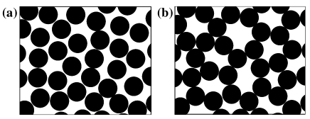
Figure 1: Schematic pictures for granular configurations: a relaxed state(a) and a jammed state(b).

For a given flow field $\mbox{\boldmath$v$}(\mbox{\boldmath$r$})$, we assume that there exists a stationary value $\phi_{*}$, toward which the state variable $\phi$ changes as

$$\tau\,{D\phi\over Dt}=-\Bigl{(}\phi-\phi_{*}\Bigr{)}$$ (6)

with the time scale $\tau$.

We may assume that $\tau$ is constant in the case where the internal state changes due to the thermal fluctuation or some other mechanism independent of the flowing field. However, we adopt the variable time scale $\tau$ that is inversely proportional to the local shear rate $\dot{\Gamma}$,

$$\tau=r\,\dot{\Gamma}^{-1}$$ (7)

with a dimensionless constant $r$, because it is more natural to suppose that the state change is driven by the flow deformation. Note that this form of $\tau$ does not introduce a new time scale to the system and makes it respond quite peculiarly to an external impact.

The stationary value $\phi_{*}$ is determined by the local flow and we assume that it is an increasing function of the local stress $S$. We employ a simple form

$$\phi_{*}(S)=\phi_{M}\cdot{(S/S_{0})^{2}\over 1+(S/S_{0})^{2}}$$ (8)

with the characteristic shear stress $S_{0}$. The parameter $\phi_{M}$ represents the value of the state variable in the high stress limit and should depend upon the volume fraction of the granules and some other parameters of the medium.

For the scalar values of the shear rate $\dot{\Gamma}$ and the shear stress $S$ in Eqs.(7) and (8), we adopt the definitions

$$\dot{\Gamma}\equiv\sqrt{{1\over 2}\,\mathrm{Tr}[\hat{\dot{\gamma}}\cdot\hat{\dot{\gamma}}]},\quad S\equiv\sqrt{{1\over 2}\,\mathrm{Tr}[\hat{\sigma}\cdot\hat{\sigma}]},$$ (9)

which reduce to the ordinary shear rate and shear stress in the case of simple shear flow.

Viscosity:

The shear thickening property of the model comes from the $\phi$-dependence of the viscosity, for which we assume

$$\eta(\phi)=\eta_{0}\exp\left[A{\phi\over 1-\phi}\right]$$ (10)

with the viscosity in the relaxed state $\eta_{0}$ and a dimensionless parameter $A$. We have introduced the Vogel-Fulcher type strong divergence at the jamming point $\phi=1$ in order to represent severe thickening observed in the dilatant fluid. In Eq.(10), the state variable $\phi$ plays an analogous role with the inverse temperature in the glass transition. Note that the state variable $\phi$ cannot be $\phi>1$ even when $\phi_{M}>1$ in Eq.(8) if we employ Eq.(7) because the shear rate vanishes $\dot{\Gamma}\searrow 0$ as $\phi\nearrow 1$ due to the diverging viscosity.

Unit system:

For numerical presentation, we employ the unit system where

$$\eta_{0}=S_{0}=\rho=1,$$ (11)

namely, the time, length, and mass are measured by the units

$$\tau_{0}\equiv{\eta_{0}\over S_{0}},\qquad\ell_{0}\equiv\sqrt{{\eta_{0}\over\rho}\,\tau_{0}},\qquad m_{0}\equiv\rho\,\ell_{0}^{3},$$ (12)

respectively. The rate $1/\tau_{0}$ gives the scale for the shear rate where thickening occurs, and the length scale $\ell_{0}$ is the corresponding hydrodynamic length scale. For the cornstarch suspension of 41 wt%Fall et al. (2008), these parameters may be estimated as $S_{0}\approx 50\,{\rm Pa}$, $\eta_{0}\approx 10\,{\rm Pa\cdot s}$, and $\rho\approx 10^{3}\,{\rm kg/m^{3}}$, which give $\tau_{0}\approx 0.2\,{\rm s}$ and $\ell_{0}\approx 5\,{\rm cm}$.

III Simple shear flow under external shear stress

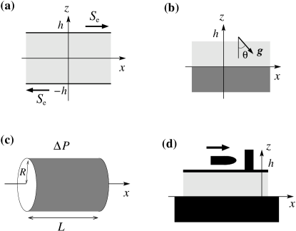
Figure 2: Simple flow configurations and the coordinate system: (a) shear flow, (b) gravitational slope flow, (c) Poiseuille flow, and (d) impact by a bullet.

First, we will study behaviors of the dilatant fluid for a simple shear flow under an externally applied shear stress(Fig. 2(a)). The velocity field is assumed to be $\mbox{\boldmath$v$}=(u(z,t),0,0)$ and the external stress imposes the boundary condition

$$S(z,t)\Bigr{|}_{z=\pm h}=S_{\rm e},$$ (13)

where we have introduced the notation for the shear stress

$$S(z,t)\equiv\eta(\phi)\;\dot{\gamma}(z,t)$$ (14)

with the shear rate

$$\dot{\gamma}(z,t)\equiv{\partial u(z,t)\over\partial z}.$$ (15)

$h$ is the half width of the flow and $S_{\rm e}$ is the applied stress at the boundaries(Fig. 2(a)). Then, Eqs.(1) and (6) become

$$\rho{\partial u(z,t)\over\partial t} = {\partial\over\partial z}S(z,t),$$ (16)

$$r{\partial\phi(z,t)\over\partial t} = -|\dot{\gamma}(z,t)|\Bigl{(}\phi(z,t)-\phi_{*}\bigl{(}S(z,t)\bigr{)}\Bigr{)},$$ (17)

In the following, we first examine a steady flow solution, then perform the stability analysis for the solution and the numerical simulation for these equations of motion.

III.0.1 Steady flow solution

The steady solution for Eqs.(13) $\sim$ (17) can be readily obtained as

$$\phi=\phi_{*}(S_{\rm e}),\quad\dot{\gamma}={S_{\rm e}\over\eta\bigl{(}\phi_{*}(S_{\rm e})\bigr{)}}\equiv\dot{\gamma}_{*}(S_{\rm e}).$$ (18)

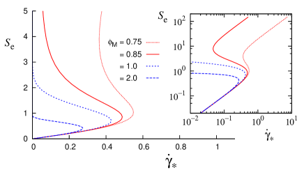
Figure 3: (Color online) The stress-shear rate relation for the viscosity given by Eq.(18) for various $\phi_{M}$ with $A=1$. The inset shows the plots in the logarithmic scale.

From these equations, we can obtain the relationship between the stress and the shear rate, which is plotted in Fig.3 for various values of $\phi_{M}$ with $A=1$. In the logarithmic plots, the straight line with the slope 1 correspond to the linear stress-shear rate relation with a constant differential viscosity. One can see that there are two regimes: the low viscosity regime in the low shear stress and the high viscosity regime in the high shear stress. Between the two regimes, there is a branch where the shear rate decreases for increasing shear stress. The state in the middle branch can be unstable against infinitesimal perturbation.

From this stress-shear rate relation, we expect there should be hysteresis upon changing the shear rate; if the system starts from the low shear rate on the lower branch, the stress increases continuously, but before the system reaches the end of the lower branch, it should jump to the upper branch by discontinuous increase of the stress. If the system starts from the high shear rate on the upper branch and the shear rate decreases, the stress should jump to the lower branch before the system reaches the end of the upper branch. This sudden increase/decrease of stress corresponds to the discontinuous change of viscosity in the shear thickening.

III.0.2 Linear stability of the steady flow

Now, we examine the linear stability of the steady shear flow given by Eq.(18). For a full analysis, an arbitrary perturbation should be allowed, but here we examine the linear stability against the restricted perturbation where the velocity is in the $x$-direction and the spatial dependence is only on the $z$ coordinate:

$$\mbox{\boldmath$v$}(\mbox{\boldmath$r$},t)=(\dot{\gamma}_{*}z+\delta u(z,t),0,0),\qquad\phi(\mbox{\boldmath$r$},t)=\phi_{*}(S_{\rm e})+\delta\phi(z,t),$$ (19)

then the dynamics is analyzed using Eqs.(16) and (17). Even within this restriction, we will see the steady shear flow in the middle branch may become unstable and the oscillatory flow arises.

The linearized equations for the perturbation are now given by

$$\rho\,{\partial\over\partial t}\delta\dot{\gamma}(z,t) = \eta_{*}{\partial^{2}\over\partial z^{2}}\delta\dot{\gamma}(z,t)+\eta_{*}^{\prime}\dot{\gamma}_{*}{\partial^{2}\over\partial z^{2}}\delta\phi(z,t),$$ (20)

$$r\,{\partial\over\partial t}\delta\phi(z,t) = \dot{\gamma}_{*}\Bigl{(}\phi_{*}^{\prime}\,\eta_{*}\delta\dot{\gamma}(z,t)+\bigl{(}-1+\phi_{*}^{\prime}\eta_{*}^{\prime}\dot{\gamma}_{*}\bigr{)}\delta\phi(z,t)\Bigr{)},$$ (21)

where the primes denote the derivative by its argument, and we have introduced the abbreviated notations,

$$\eta_{*}\equiv\eta\bigl{(}\phi_{*}(S_{\rm e})\bigr{)},\quad\eta_{*}^{\prime}\equiv\left.{d\eta(\phi)\over d\phi}\right|_{\phi=\phi_{*}(S_{\rm e})},\quad\phi_{*}^{\prime}\equiv{d\phi_{*}(S_{\rm e})\over dS_{\rm e}}.$$ (22)

Then, the growth rate $\Omega_{k}$ of the perturbation for the Fourier component with the wave number $k$ in the $z$ direction is determined by

$$\left|\begin{array}[]{cc}\rho\Omega_{k}+k^{2}\eta_{*},&k^{2}\eta_{*}^{\prime}\dot{\gamma}_{*}\\ -\dot{\gamma}_{*}\phi_{*}^{\prime}\,\eta_{*},&r\Omega_{k}-\dot{\gamma}_{*}\bigl{(}-1+\phi_{*}^{\prime}\eta_{*}^{\prime}\dot{\gamma}_{*}\bigr{)}\end{array}\right|=0.$$ (23)

This gives a positive real part of $\Omega_{k}$ for the wave number $k$ that satisfies

$$0<k^{2}<k_{c}^{2}\equiv{1\over r}\,\left({\rho\over\eta_{*}}\right)S_{\rm e}\left(-{d\dot{\gamma}_{*}\over dS_{\rm e}}\right)$$ (24)

in the case $d\dot{\gamma}_{*}/dS_{\rm e}<0$, i.e. $S_{\rm e}$ is in the unstable branch of the shear stress-shear rate curve. Since the smallest possible wave number $k$ for the perturbation is $\pi/(2h)$ and $\eta_{*}/\rho$ is the kinematic viscosity for the steady flow, we can interpret this result in the way that the steady shear flow in the unstable branch is unstable as long as the system width is larger than the momentum diffusion length due to the viscosity.

For a given external shear stress $S_{\rm e}$ in the unstable branch, the flow becomes unstable for the system wider than $2h_{c}\equiv\pi/k_{c}$, where the growth rate $\Omega_{k}$ has a finite imaginary part $\omega_{c}$ given by

$$\omega_{c}\equiv\sqrt{S_{\rm e}\over r\rho}\;k_{c}={1\over r}\sqrt{S_{\rm e}\left(-{d\dot{\gamma}_{*}\over dS_{\rm e}}\right)\dot{\gamma}_{*}}.$$ (25)

Note that the scales of $k_{c}$ and $\omega_{c}$ are typically set by $1/\ell_{0}$ and $1/\tau_{0}$ although their actual values depend on $r$ and the other system parameters, i.e. $A$ and $\phi_{M}$.

III.0.3 Shear thickening oscillation in unstable shear flow

The oscillatory behavior of the shear flow in the unstable regime can be seen by numerically integrating Eqs.(16) and (17) with Eqs.(14) and (15). In Fig.4, the average shear rates $u(h)/h$ for (anti-)symmetric solutions are plotted as a function of time for various system width $h$ with the constant shear stress $S_{\rm e}=1.1$ in the unstable regime for $A=\phi_{M}=1$ and $r=0.1$. The initial state is prepared as the steady solution (18) for $S_{\rm e}=1$. For this set of parameters, $k_{c}=1.18$, which gives $h_{c}=1.33$ and $\omega_{c}=3.91$.

For $h=1.3$, which is smaller than $h_{c}$, the flow shows overdumped sinusoidal oscillation with the angular frequency 4.0, which is close to $\omega_{c}$. For larger $h$, the oscillation becomes self-sustained and non-linear; the gradual buildups of the flow speed are followed by sudden drops.

This non-linear oscillation of shear thickening fluid is shown in more detail in Fig.5, where the time development of the $\phi(z)$ and $u(z)$ are plotted. Only the positive half of the solution is plotted for the (anti-)symmetric solution. In the plots, the oscillation starts from the almost uniform shear flow in the high viscosity state with a larger value of $\phi$. This flow cannot be completely uniform because the external shear stress $S_{\rm e}$ is in the unstable branch, thus the flow speed builds up gradually as the internal state $\phi$ relaxes to reduce the viscosity, but eventually, $\phi$ starts increasing when the shear stress becomes large enough. Then, larger value of $\phi$ causes higher viscosity, which decelerates the flow speed, but this causes even higher value of $\phi$ because the inertia stress due to the deceleration is added on the top of the stress by the shear flow, which results in the sudden drop of the flow speed.

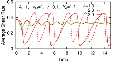
Figure 4: (Color online) Oscillation of the average shear rate $u(h)/h$ in the shear flow for $h=1.3$, 2, and 3 with $A=\phi_{M}=1$, $r=0.1$, and $S_{\rm e}=1.1$. The (green) line, that overlaps the plot for $h=1.3$, shows the plot for $f(t)=c_{1}+c_{2}\,e^{-t/\tau}\sin(\omega t+\theta)$ with $\omega=4.0$, $\tau=5.8$, $\theta=0.86$, $c_{1}=0.33$, and $c_{2}=0.056$.

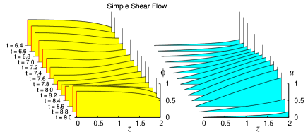
Figure 5: (Color online) Time development of $\phi(z)$ (left) and $u(z)$ (right) in the shear flow oscillation for $A=\phi_{M}=1$, $r=0.1$, $S_{\rm e}=1.1$, and $h=2$. Only the positive parts of the flow ($z>0$) are presented.

IV Gravitational slope flow and Poiseuille flow

Similar analyses are performed for a gravitational slope flow and Poiseuille pipe flow.

IV.1 Gravitational slope flow

For the gravitational slope flow (Fig.2(b)), Eqs.(1) and (6) should be solved with the boundary conditions

$$\mbox{\boldmath$v$}\bigr{|}_{z=0}=0,\qquad\hat{\sigma}\cdot\mbox{\boldmath$n$}\bigr{|}_{z=h(x,y)}=0,$$ (26)

where we have assumed that the bottom of the flow is located at $z=0$ and the flow depth at $(x,y)$ is given by $h(x,y)$; the vector $n$ represents the normal vector to the flow surface. The gravitational body force is given by

$$\mbox{\boldmath$g$}=(g\sin\theta,0,-g\cos\theta)\equiv(g_{\parallel},0,-g_{\perp})$$ (27)

with the slope angle $\theta$.

For the flow field $\mbox{\boldmath$v$}=(u(z,t),0,0)$, Eqs.(1) and (6) become

$$\rho\;{\partial u(z,t)\over\partial t} = {\partial S(z,t)\over\partial z}+g_{\parallel},$$ (28)

$$0 = -{\partial P(z)\over\partial z}-g_{\perp},$$ (29)

$$r{\partial\phi(z,t)\over\partial t} = -|\dot{\gamma}(z,t)|\Bigl{(}\phi(z,t)-\phi_{*}\bigl{(}S(z,t)\bigr{)}\Bigr{)}$$ (30)

with the shear stress (14) and the boundary conditions (26) are given by

$$u(0)=0,\qquad\left.{\partial u(z,t)\over\partial z}\right|_{z=h}=0.$$ (31)

Eq.(29) can be solved immediately to give the pressure

$$P(z)=g_{\perp}(h-z)+P_{0}$$ (32)

with the atmospheric pressure $P_{0}$.

The steady solution for Eqs.(28) and (30) under the boundary condition (31) is given by

$$\phi(z)=\phi_{*}\bigl{(}S_{g}(z)\bigr{)},\quad\dot{\gamma}(z)={S_{g}(z)\over\eta\Big{(}\phi_{*}\bigl{(}S_{g}(z)\bigr{)}\Big{)}}$$ (33)

with the gravitational shear stress

$$S_{g}(z)\equiv g_{\parallel}(h-z).$$ (34)

From these, the flow speed $u(z)$ and the flux per unit width $\Phi_{G}$ can be calculated by

$$u(z)=\int_{0}^{z}\dot{\gamma}(z^{\prime})\,dz^{\prime},\quad\Phi_{G}=\int_{0}^{h}u(z)dz.$$ (35)

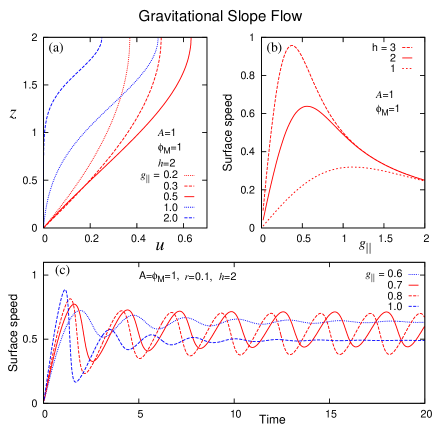
Figure 6: (Color online) Steady Gravitational flows: (a) the flow speed profiles as a function of $z$, (b) the surface flow speed vs $g_{\parallel}$, and (c) the time development of the surface speed.

In Fig.6, the flow speed profiles and the surface speeds given by Eq.(35) plotted for several sets of parameters. The depth dependences of the flow speed are shown in Fig.6(a) for some values of $g_{\parallel}$; For small $g_{\parallel}$, the flow speed depends upon the depth parabolically as in a Newtonian fluid, while, for larger $g_{\parallel}$, the flow speed profile develops a convex part, which corresponds with the unstable branch of Fig.3 in the shear flow. In Fig.6(b), the surface speed $u(h)$ are plotted as a function of $g_{\parallel}$ for some values of $h$. One can see they decreases for large $g_{\parallel}$, which means that the fluid flows slower for larger inclination angle. This is because the viscosity of the fluid becomes large in the high shear stress caused by large $g_{\parallel}$.

IV.2 Poiseuille Flow

Pressure driven pipe flow with the cylindrical symmetry around the $x$-axis (Fig.2(c)) is governed by the equation

$$\rho\,{\partial u(r,t)\over\partial t} = +{\Delta P\over L}+{1\over r}\,{\partial\over\partial r}\Bigl{(}rS(r,t)\Bigr{)},$$ (36)

$$r{\partial\phi(r,t)\over\partial t} = -|\dot{\gamma}(r,t)|\Bigl{(}\phi(r,t)-\phi_{*}\bigl{(}S(r,t)\bigr{)}\Bigr{)}$$ (37)

with the shear stress and the shear rate

$$S(r,t)=\eta(\phi)\dot{\gamma}(r,t),\quad\dot{\gamma}(r,t)={\partial u(r,t)\over\partial r}.$$ (38)

Here, $\Delta P$ ($>0$) is the pressure drop along the pipe over the length $L$, and $r$ is the distance from the central axis: $r\equiv\sqrt{y^{2}+z^{2}}$.

The steady flow solution for this configuration is given by

$$\phi(r)=\phi_{*}(S_{P}(r)),\quad\dot{\gamma}(r)={S_{P}(r)\over\eta\Bigl{(}\phi_{*}\bigl{(}S_{P}(r)\bigr{)}\Bigr{)}}$$ (39)

with the Poiseuille shear stress

$$S_{P}(r)\equiv-\,{1\over 2}\,{\Delta P\over L}r.$$ (40)

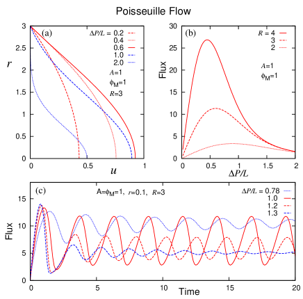
Figure 7: (Color online) Poiseuille flow: (a) the flow speed profiles as a function of $r$, (b) the flow flux vs pressure gradient $\Delta P/L$, and (c) the time development of the flux.

In Fig.7, the flow speed profiles $u(r)$ and the flow flux $\Phi$ defined as

$$\Phi\equiv\int_{0}^{R}u(r)2\pi r\,dr$$ (41)

are plotted. General features of the flow is analogous to those of the gravitational flow, and the flow flux decreases upon increasing the pressure gradient for the large pressure gradient because of the shear thickening.

IV.3 Shear thickening oscillation in gravitational flow and Poiseuille flow

These steady flows become unstable when the shear stress is in the range of the unstable branch at some region of the flow. The oscillations in the surface flow speed and the flow flux are plotted for the gravitational and Poiseuille flow in Figs.6(c) and 7(c), respectively. The shear thickening oscillation appears in a large enough system for a certain range of external drive $g_{\parallel}$ or $\Delta P/L$; The system length scale should be larger than the viscous length scale of the flow, and the external drive should be in the range where some part of the flow is in the unstable branch. From the plots, one can see the oscillation disappears when the external drive is either too small or too large. In the former case, the fluid behaves as Newtonian while in the latter case the size of the unstable region becomes too small. The shape of the oscillation in the non-linear oscillation regime is saw-teeth like, i.e. gradual increases followed by sudden drops, as we have discussed in the simple shear flow case.

The spatial variation of oscillatory flow are shown in Fig.8. The general feature is the same with that of the shear flow, but the value of $\phi$ is zero at the surface of the gravitational flow and at the center of Poiseuille flow because the shear is zero.

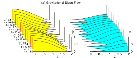
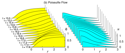
Figure 8: (Color online) Time development of $\phi(z)$ (left) and $u(z)$ (right) in the oscillatory flow of the gravitational slope flow (a) and the Poiseuille flow (b). The parameters are $A=\phi_{M}=1$ and $r=0.1$ with $g_{\parallel}=0.8$ and $h=2$ for the gravitational flow and with $\Delta P/L=1$ and $R=3$ for Poiseuille flow.

V Response to an external impact

One of the peculiar features of the dilatant fluid is instantaneous hardening by an external impact. It hardens almost immediately upon application of an external impact and allows little deformation like rigid material. It has been demonstrated that the hardening is so rapid that the material can be used for a body armor to stop a bulletWagner and Brady (2009). Such instantaneous hardening cannot be explained by the transformation between steady configurations of granules, but must be a result of the failure to rearrange the granular configuration due to some obstruction. Upon sudden impact, the granules are inhibited to rearrange their configurations due to to either dissipation by the interstitial fluid or the jamming by direct contacts. In the case of slow deformation, the stress is low and the lubrication due to the fluid allows the granules to re-arrange themselves so that they can pass each other.

In the present model, this aspect of the medium is represented by Eq.(7) that the relaxation rate of the internal state is proportional to the shear rate. For a sudden deformation, the state variable changes to a high stress value as the medium deforms; When the medium is dense ($\phi_{M}\gtrsim 1$) and the external impact is strong enough, the state reaches the jammed state after a certain amount of deformation, which is almost independent of the speed of deformation.

In order to demonstrate this aspect of the model, we perform simple simulations that the layer of fluid of the thickness $h$ is driven by a sudden motion of the upper boundary wall at $z=h$ with the fixed lower boundary at $z=0$ (Fig.1d). Let $U(t)\equiv u(h,t)$ be the velocity of the upper wall. Initially, the fluid is at rest,

$$u(z,t)=0,\quad\phi(z,t)=0,\quad U(t)=0\quad\mbox{for $t<0$},$$ (42)

then the upper wall is moved suddenly by the velocity $u_{0}$ at $t=0$, $U(0)=u_{0}$. For $t>0$, the velocity of the upper wall is determined by

$$m{dU(t)\over dt}=-\eta\bigl{(}\phi(h,t)\bigr{)}{\partial u(z,t)\over\partial z}\Bigr{|}_{z=h},$$ (43)

with Eqs.(16) and (17), where $m$ is the mass of the upper wall per unit length.

Fig.9 shows the displacement $X(t)$ of the upper wall,

$$X(t)=\int_{0}^{t}U(t^{\prime})dt^{\prime},$$ (44)

for the three cases, $\phi_{M}=0.8$, 1, and 2 for various initial speeds $u_{0}$ increases. The wall decelerates rapidly as the fluid thickens in response to the stress, and eventually stops. For $\phi_{M}=0.8$, the final wall displacement increases as the initial speed $u_{0}$. On the other hand, for $\phi_{M}=1$ and 2, the final displacement hardly depend on $u_{0}$ when $u_{0}>5$. This is because the fluid gets jammed at a certain strain as it deforms, and cannot deforms further. However, when the initial speed is small enough, the upper wall does not stop quickly because the fluid does not thicken as shown Fig.9(c).

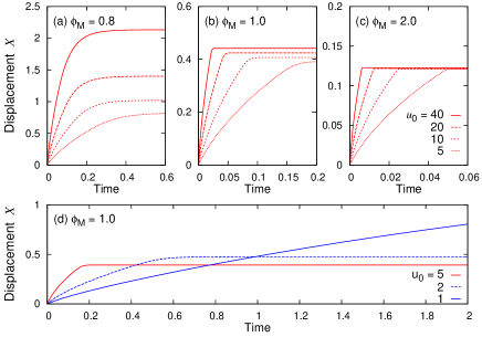
Figure 9: (Color online) The time dependence of the displacement $X$ after the impact for the system of $\phi_{M}=0.8$ (a), 1 (b), and 2 (c) with the initial speed $u_{0}=40$, 20, 10, and 5, and for the system of $\phi_{M}=1.0$ with $u_{0}=5$, 2, and 1 (d). The other parameters are $h=2$, $r=0.1$, and $A=m=1$.

VI Two dimensional inhomogeneous flow

Now, we present the results of numerical simulations for two dimensional system in the simple shear configuration (Fig.2(a)) in order to examine how the inhomogeneity in the $x$ direction affects the system behavior, especially in the case of shear thickening oscillation.

The velocity field is assumed to be in the $x-z$ plane, $\mbox{\boldmath$v$}=(u(x,z,t),0,w(x,z,t))$, and in the $x$ direction we employ the periodic boundary condition with the system length $L$. We take $L=10h$ in the present simulations.

The fluid dynamic equation (1) is integrated using the standard MAC(Marker-and-Cell) methodHarlow and Welch (1965) for the incompressible fluid, and $|\mbox{\boldmath$\nabla$}\cdot\mbox{\boldmath$v$}|$ is kept less than $10^{-10}$. Euler method is employed for the time integration of Eqs.(1) and (6).

The motion of the plates at $z=\pm h$ is controlled so that the average shear stress on the plate is equal to $S_{\rm e}$,

$${1\over L}\int_{0}^{L}\eta\bigl{(}\phi(\mbox{\boldmath$r$},t)\bigr{)}\dot{\gamma}_{xz}(\mbox{\boldmath$r$},t)\Bigr{|}_{z=\pm h}dx=S_{\rm e}.$$ (45)

As for the initial configuration at $t=0$, we assume that the fluid is at rest and the state variable $\phi$ is close to zero with small fluctuations introduced at every computational grid point $\mbox{\boldmath$r$}_{i}$,

$$\mbox{\boldmath$v$}(\mbox{\boldmath$r$},0)=0,\quad\phi(\mbox{\boldmath$r$}_{i},0)=\xi_{i},$$ (46)

where $\xi_{i}$ is a random variable uniformly distributed over $[0,\epsilon)$ with a small parameter $\epsilon$. We take $\epsilon=10^{-4}$. Note that, for the case of $\epsilon=0$, all quantities do not depend on $x$, thus the simulations reduce to the one dimensional case given in Sec. III.

VI.1 Flow diagrams

Fig.10 shows a flow diagram in the $S_{\rm e}-h$ plane for $\phi_{M}=0.85$ with $A=1$ and $r=0.1$ (the inset for $\phi_{M}=1$). The diagrams are determined by the simulations at the points with marks.

In the steady shear flow (grey) and the oscillatory flow (purple) regions, the initial fluctuations do not grow, thus the flows remain homogeneous in the $x$ direction and are the same with those in the corresponding one dimensional cases in Sec.III (Fig.11); the dashed lines show the boundary for the two regimes in the one-dimensional case given by

$$k_{c}(S_{\rm e})={\pi\over 2h}$$ (47)

using the definition of $k_{c}$ in Eq.(24) as a function of $S_{\rm e}$. In the low $S_{\rm e}$ side, one can see that this coincides with the corresponding boundary in the two-dimensional case between the steady shear flow and the oscillatory flow.

The major difference between the one and the two dimensional cases is that these two homogeneous flow regimes are limited to the smaller $S_{\rm e}$ side. In the larger $S_{\rm e}$ region, the initial fluctuations in the state variable $\phi$ grows, thus the flow results in the inhomogeneous flow in the case of $\phi_{M}=0.85$(pink) or the jammed flow in the case of $\phi_{M}=1.0$ of the inset. In the following, we examine the flows in these two regimes.

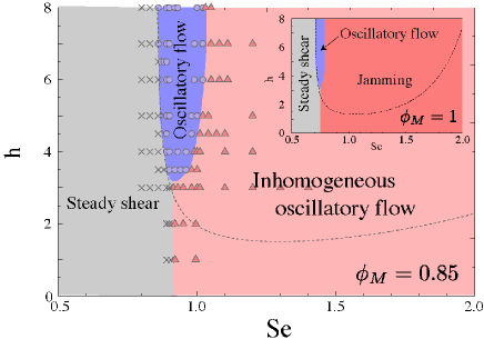
Figure 10: (Color online) Flow diagram of the shear flow for $\phi_{M}=0.85$. The internal state variable $\phi$ does not depend on $x$ in the region colored with gray and blue. The inset is the same diagram obtained for $\phi_{M}=1$. The other parameters are $A=1$, $r=0.1$, with $L=10h$.

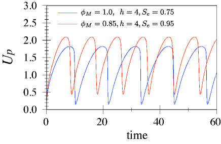
Figure 11: (Color online) Time development of the upper plate velocity $U_{p}$ in the oscillatory flow regime in the two-dimensional simulation. The initial fluctuations decay quickly and the flows show homogeneous oscillation as in the case of the one-dimensional system.

VI.2 Inhomogeneous oscillatory flow

First, we examine the flow for $\phi_{M}=0.85$. In this case, the viscosity does not diverge and the medium keeps flowing. In Fig.12, the time evolution of the upper plate velocity $U_{p}$ is plotted along with the case without initial fluctuations. The flow shows irregular oscillation with smaller amplitude compared with the noiseless case.

The snapshots of $\phi$ for a single cycle of oscillation in Fig.13 reveal that the whole system is not thickened and the oscillation is governed by a few thickening bands. At the time when $U_{p}$ reaches its minimum (a), the thickening branch with the high value of $\phi$ (the red region) is being extended along the direction of $(1,1)$. As the system flows, this branch is stretched and $U_{p}$ gradually increases (b), and eventually the branch breaks off and $U_{p}$ reaches maximum (c). Then, high shear rate makes the broken branches extend again to the other side to cause sudden deceleration (d). The thickening branches first appear both in $(1,1)$ and $(1,-1)$ direction, but the latter tend to disappear and transforms into the $(1,1)$ direction in the course of time, and only the thickening branches in the $(1,1)$ direction remain.

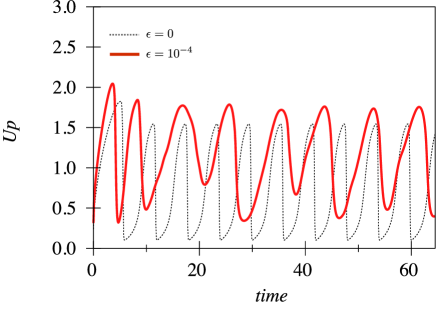
Figure 12: (Color online) The time evolution of the upper plate velocity $U_{p}$ in the inhomogeneous oscillatory flow regime with $\phi_{M}=0.85$. The other parameters are $h=5$, $L=50$, $S_{\rm e}=1.5$, $A=1$, and $r=0.1$. The initial fluctuation is given by $\epsilon=10^{-4}$. The uniform oscillation flow with $\epsilon=0$ (the dashed line) is shown for comparison.

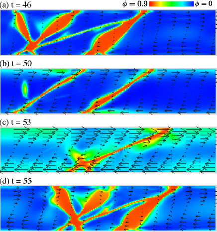
Figure 13: (Color online) The snapshots of the state variable $\phi$ taken during a cycle of oscillation presented in Fig.12. The arrows indicate flow velocity.

VI.3 Jamming caused by the instability

For the case of $\phi_{M}=1$, the viscosity can diverges and the instability of the homogeneous flow causes the jamming to stop the flow.

Figs.14 and 15 shows the simulation results for $\phi_{M}=1$. The time evolution of the viscosity distribution at $z=0$ is shown in Fig.14. Initially, the viscosity is rather uniform with some fluctuations, but peak structure appears soon around $t=3$ with a certain characteristic length scale. Some of the peaks grow sharply and the thickening regions strongly localize($t\gtrsim 4$), then the system is jammed and the flow stops within a period of oscillation of the homogeneous case(Fig.16).

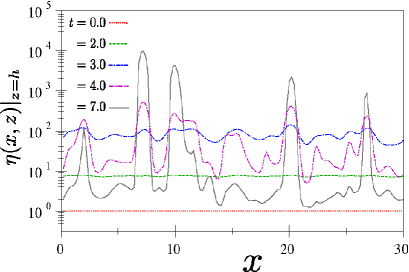
Figure 14: The spatial variation of viscosity $\eta$ at $z=0$ at several times in the jamming regime. The parameters are $h=3$, $L=30$, $S_{\rm e}=1.5$, $\phi_{M}=1$ with $A=1$ and $r=0.1$.

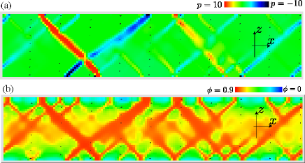
Figure 15: (Color online) (a) The spatial distribution of the pressure $P$ and (b) the internal state variable $\phi$ in the system presented in Fig.14 at t = 4.

Fig.15 shows the color maps of the pressure $P$ (a) and the state variable $\phi$ (b) at $t=4$. The fluctuation of $\phi$ first stands out just below the moving plates, but higher $\phi$ regions form band structure, and extend along the principal axis of the shear deformation, $(1,1)$ and $(1,-1)$. Some of the bands reach the upper plate from the lower plate, and they jam the system.

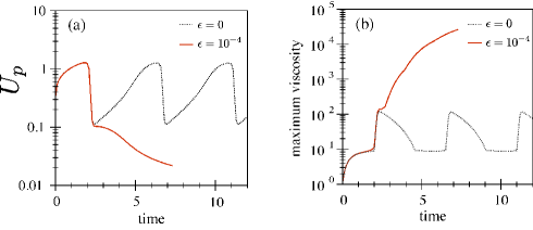
Figure 16: (Color online) The time evolution of (a) the upper plate velocity $U_{p}$, and (b) the maximum viscosity in the system presented in Fig.14. The dashed lines represent the oscillatory flow without fluctuations.

In Fig.16(a), we present the velocity of upper plate $U_{p}$ as a function of time. The solid line shows the time evolution starting from the internal state with fluctuations, and the dotted line represents the case without fluctuations for comparison. The state variable suddenly loses homogeneity at $t=2.3$, then thickening branches appears, and the velocity $U_{p}$ drops to zero. The maximum viscosity is always found inside the thickening branch for $t\gtrsim 2.3$, and its value sharply increases as plotted in Fig.16(b). We cannot simulate the system up to the time when the plates motion actually stops because the numerical time integration becomes difficult as the viscosity becomes large, since it requires smaller time step. In the present case, however, we expect the system is jammed because the decrease of $U_{p}$ and the increase of maximum viscosity are rapid and monotonic.

VII Summary and Discussions

The shear thickening shown by a dense mixture of granules and fluid has some peculiar features: (i) instantaneous hardening, (ii) fast relaxation to flowing state, (iii) rigid thickened state, (iv) hysteretic thickening transition, (v) oscillatory flowing behavior. We constructed a fluid dynamics model by introducing a phenomenological state variable and showed that the model can describe these features. Especially, we demonstrated that the shear thickening oscillation appears in various shear flow configurations.

Comparison with visco-elasticity:

A visco-elastic fluid such as a polymer melt shows analogous behavior to the dilatant fluid; It behaves like a solid in a short time scale and like a fluid in a long time scale. This may be compared with that of the dilatant fluid, i.e. instantaneous hardening in response to an external impact and fluidization after relaxation of the applied stress. However, there are some important differences; the visco-elastic medium changes its behavior according to the observation time scale, and it also allows large elastic deformation even in a short time solid like behavior. On the other hand, the dilatant fluid changes its behavior according to the stress, i.e. it stays hardened while it is under the stress and starts flowing within a few second after the removal of the applied stress. The dilatant fluid allow little deformation even under large stress.

Shear stress thickening:

In constructing the model, we assume the fluid is shear-stress thickening, i.e. the viscosity depends upon the state variable $\phi$, and the steady value of the state variable $\phi_{*}$ is determined by the local stress as in Eq.(8). It is instructive to see what would happen if we assume $\phi_{*}$ as a function of the shear rate $\phi_{*}(\dot{\gamma})$. In this case, the viscosity is directly given as a function of the shear rate, $\eta\bigl{(}\phi_{*}(\dot{\gamma})\bigr{)}$, thus we should not have a discontinuous thickening unless we assume a discontinuity either in $\phi_{*}(\dot{\gamma})$ or in $\eta(\phi)$.

Experimentally, the most direct evidence for the shear-stress thickening should be obtained by the observation that the pipe flow flux is not monotonically increasing as a function of the applied pressure gradient.

State variable:

Although we introduced the state variable $\phi$ phenomenologically, we suppose that the variable represents a certain microscopic property of the medium, such as contact numbers between grains, associated with the restrictions against local rearrangement of granular configuration. The variable could be a vector or a tensor, but we examined the scalar case for simplicity. It is notable that even the scalar state variable produces the anisotropic stress chain like structure in the system as we have seen in the two-dimensional simulations.

Jamming and response to impact:

A remarkable feature of the dilatant fluid is that hardening response is so instantaneous that the medium can be used for a body armor to stop a bulletWagner and Brady (2009). We believe that such an instantaneous severe hardening cannot be explained by a transformation between two steady states, i.e. from the fluid state under low stress to the rigid state under high stress. Instead, it must be a result that the rapid rearrangement in the granular configuration is inhibited. There are two possible mechanisms that inhibit the granular rearrangement in the densely packed medium: the Reynolds dilatancy and the formation of stress chains. The Reynolds dilatancy can inhibit rearrangement by the fluid friction because the rearrangement should induce the strong interstitial fluid flow through granules in order to compensate the local volume change caused by the dilatancy. The stress chains through direct contacts between granules can be formed by the application external stress and prevent granules from being rearranged.

In the present model, such an aspect of hardening is represented by the fact that the relaxational time scale for the state change is not constant but proportional to the shear rate (7). Then, the state variable $\phi$ reaches a steady value $\phi_{*}$ in a time scale where the strain changes by the amount $r$. Consequently, the medium with $\phi_{M}\gtrsim 1$ can deform only up to a certain strain around $r$ by a hard impact.

Shear thickening oscillation:

One of interesting results of the present model is the shear thickening oscillation. The steady shear flow is unstable when the flow is in the unstable branch of the shear stress-shear rate curve and is wide enough compared to the diffusion length scale by the viscosity. In this case, the flow shows the oscillation between the thick state in the high shear regime and the thin state in the low shear regime. In two dimensions, uniform oscillation appears only in the smaller external shear stress region, but some oscillatory behavior remains even when inhomogeneity develops in the flow.

The shear thickening oscillation in the homogeneous flow looks similar to the stick-slip motion in a frictional system. However, there are some important differences; the stick-slip motion starts with the sudden acceleration caused by the slip weakening resistance under the constant speed driving through a mechanism with finite rigidity, while the shear thickening oscillation starts with the sudden deceleration caused by the shear thickening transition under the constant force driving.

Aradian and Cates have also studied the dynamics of shear thickening fluids and found oscillatory behaviorsAradian and Cates (2006). They focused, however, on the regime where the structural relaxation time is much larger than the fluid dynamical time scale, which is appropriate for liquid crystal systems. Consequently, the time scale of the oscillation is of the order or larger than the structural relaxation time scale, therefore the dynamics is completely dissipative. On the other hand, in the present case, the structural relaxation time of the state variable is set by the shear rate and always comparable with the fluid dynamical time scale, thus the period of the oscillation is determined by the fluid dynamics. It is also clear that the stress from the inertia plays an important role in the thickening phase in the oscillation.

Experiments:

As for the hysteresis, Deegan observed the hysteresis loop of the viscosity under the oscillatory stress for the cornstarch-fluid system and considered it to be the mechanism for persistent holesDeegan (2010). His system is thinner and in the regime of mild shear thickening in comparison with the system studied by Fall et alFall et al. (2008). In the present work, we try to model rather severe shear thickening in choosing the functional form of the viscosity Eq.(10), but the present model qualitatively reproduces main feature of his data, by adjusting the parameters for $\phi_{M}$ and $r$ (Fig.17 compared with Fig.5 of Deegan (2010)). For this set of the parameters, the initial noise decays, thus the one and two dimensional simulations give the same results.

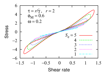
Figure 17: (Color online) Hysteresis loops in the shear stress vs the shear rate in response to oscillatory shear stress for various amplitudes. The oscillatory stress $S(t)=S_{\rm e}\sin(\omega t)$ is applied to the upper plate located at $z=h$ with the lower plate fixed at $z=0$. The system parameters are $h=0.5$, $\phi_{M}=0.6$, $r=2$, and $A=1$.

Regarding the shear thickening oscillation, we could not find any literature on the experiment which shows clear oscillation. This may partly because the system needs to be large enough, typically wider than $\ell_{0}$ or a few centimeters, and the inhomogeneity may develops in three dimensional system, which can obscure the oscillation. The noisy fluctuation often observed in rheometer experiments under constant stress may be explained by this mechanismLaun et al. (1991); Lootens et al. (2005). Nevertheless, one may easily notice the oscillation around 10 Hz simply by pouring the dense water-starch mixture out of a container. We believe that this oscillation should be explained by the shear thickening oscillation. We are planning experiments that allow quantitative comparison with our results.

Although in the different physical context, the clear oscillatory flowsWunenburger et al. (2001) along with a discontinuous transition and hysteresisBonn et al. (1998); Volkova et al. (1999) have been observed in the liquid crystal system that shows the shear thinning due to the state dependent viscosity. Such behavior could be also described using the phenomenological model like the present one.

Chaotic dynamics has been observed in dilute aqueous solutions of a surfactant in the experiment under the constant shear rate in the shear thickening regimeBandyopadhyay et al. (2000); Bandyopadhyay and Sood (2001). It was interpreted as the stick-slip transition between the two states of the fluid structure, thus physical relevance to the present instability is not clear, but we also found the chaotic dynamics in the present model in the case of the constant relaxation time $\tau$ with the large system width.