Gauge theory webs and surfaces

Abstract

We analyze the perturbative cusp and closed polygons of Wilson lines for massless gauge theories in coordinate space, and express them as exponentials of two-dimensional integrals. These integrals have geometric interpretations, which link renormalization scales with invariant distances.

I Introduction

Gauge field path-ordered exponentials Bialynicki-Birula ; Yang:1974kj ; Wilson:1974sk or Wilson lines, represent the interaction of energetic partons with relatively softer radiation in gauge theories. For constant velocities, ordered exponentials of semi-infinite length correspond to the eikonal approximation for energetic partons. Classic phenomenological applications of ordered exponentials include soft radiation limits in deeply inelastic scattering Korchemsky:1993uz and parton pair production and electroweak annihilation Korchemsky:1994is ; Belitsky:1998tc ; Kelley:2011ng . They appear as well in the treatment of parton distributions Laenen:2000ij ; Cherednikov:2013bxa . In all these cases, the electroweak current is represented by a color singlet vertex at which lines in the same color representation but with different velocities are coupled. This vertex is often referred to as a cusp.

Cusps also appear as vertices in polygons formed from Wilson lines Korchemskaya:1992je , which have been studied extensively in the context of their duality to scattering amplitudes in ${\cal N}=4$ SYM theory Drummond:2007aua ; Alday:2007hr ; Alday:2008yw ; Chien:2011wz ; Basso:2013vsa . In the strong-coupling limit of this theory, gauge-gravity duality relates the cusp and polygons to the exponentials of two-dimensional surface integrals. Surfaces bounded by open and closed paths of ordered exponentials are also a classic ingredient in lattice Wilson:1974sk and large-$N_{c}$ 'tHooft:1973jz paradigms for confinement in quantum chromodynamics.

In this paper, we show that in any gauge theory with massless vector bosons the cusp matrix element for lightlike Wilson lines can be expressed as the exponential of an integral over a two-dimensional surface, a result with applications as well to polygons formed from ordered exponentials. The corresponding integrand is an infrared finite function of the gauge theory coupling, evaluated for each point on the surface at a scale given by the invariant distance from that point to the cusp vertex. This result extends to all orders in perturbation theory.

The set of all virtual corrections for the cusp Korchemsky:1987wg is formally identical to a vacuum expectation value, and can be written as

$$\Gamma^{(f)}(\beta_{1},\beta_{2})=\bigg{\langle}0\left|T\bigg{(}\Phi^{(f)}_{\beta_{2}}(\infty,0)\,\Phi^{(f)}_{\beta_{1}}(0,-\infty)\bigg{)}\right|0\bigg{\rangle}\,,$$ (1)

in terms of constant-velocity ordered exponentials,

$$\Phi^{(f)}_{\beta_{i}}(x+\lambda\beta_{i},x) ={\cal P}\exp\left(-ig\int_{0}^{\lambda}d\lambda^{\prime}\beta_{i}\cdot A^{(f)}(x+\lambda^{\prime}\beta_{i})\right)\,.$$ (2)

Here $f$ labels a representation of the gauge group and $\beta_{i}$ is a four-velocity, taken lightlike in the following. The combination of ordered exponentials in Eq. (1) corresponds to a partonic process with spacelike momentum transfer. For correspondence to a timelike process like pair creation, $\Phi^{(f)}_{\beta_{1}}(0,-\infty)$ can be replaced by $\Phi^{(\bar{f})}_{\beta_{1}}(\infty,0)$. The imaginary parts for timelike configurations have been discussed recently in Ref. Laenen:2014jga . Corrections to partonic scattering Kidonakis:1998nf ; Bauer:2001yt ; Mitov:2009sv ; Beneke:2010da ; Ferroglia:2009ii ; Kidonakis:2010dk ; Gardi:2010rn ; Kelley:2010fn ; Jouttenus:2011wh ; Gardi:2013ita ; Gardi:2013jia involve the coupling of more than two ordered exponentials at a point Brandt:1981kf ; Korchemskaya:1994qp . In this paper we study the all-orders properties of the single cusp and of polygons with sequential cusps, computed perturbatively in coordinate space.

Perturbative corrections to the unrenormalized cusp, Eq. (1) are scaleless, and hence vanish in dimensional regularization. The ultraviolet poles of (1) determine the anomalous dimension of the cusp, and can be used to define a renormalized expansion, both for the cusp and for polygons formed from ordered exponentials of finite length Brandt:1981kf ; Korchemskaya:1992je . For the cusp in an asymptotically free theory, however, neither its ultraviolet nor its infrared behavior can be considered as truly physical. At very short distances, dynamics is perturbative and recoil cannot be neglected. At very long distances, dynamics is nonperturbative, and dominated by the hadronic spectrum. In this discussion, we will regard the cusp as an interpolation between these asymptotic regimes. We will concentrate on the structure of the integrals in the intermediate region, although we also discuss their renormalization.

We begin in Sec. II with a review of exponentiation for products of ordered exponentials, a result that extends to arbitrary products of such lines and to closed loops. Section III recalls the coordinate-space picture of exponentiation in terms of web diagrams and introduces the cancellation of subdivergences of webs. It is in this discussion that a surface interpretation of the exponent emerges. We provide a two-loop illustration of subdivergence cancellation, motivate its generalization to all orders, and give an all-orders prescription for the calculation of the cusp exponent. In Sec. IV, we apply these ideas to multi-cusp polygonal Wilson loops.

II Exponentiation and Momentum-Space Webs

The cusp has long been known Gatheral:1983cz to be the exponential of a sum of special diagrams called webs, which are irreducible by cutting two eikonal lines. We represent this result as

$$\Gamma(\beta_{1},\beta_{2},\varepsilon)\ =\ \exp E(\beta_{1},\beta_{2},\varepsilon)\,,$$ (3)

in $D=4-2\varepsilon$ dimensions. The exponent $E$ equals a sum over web diagrams, $d$, each given by a group factor multiplied by a diagrammatic integral,

$$E(\beta_{1},\beta_{2},\varepsilon)\ =\ \sum_{webs\ d}\overline{C}_{d}\;{\cal F}_{d}(\beta_{1},\beta_{2},\varepsilon)\,,$$ (4)

where ${\cal F}_{d}$ represents the momentum- or coordinate-space integral for diagram $d$. The coefficients of these integrals, $\overline{C}_{d}$ are modified color factors. Two-loop examples are shown in Fig. 1.

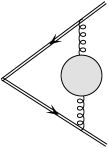
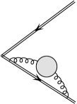
Figure 1: Two-loop web diagrams, referred to in the text as: 1 $E_{\rm cross}$, 1 $E_{3g}$, 1–1 $E_{\rm se}$. Web diagram 1 has the modified color factor, $C_{a}C_{A}/2$, where $a$ refers to the representation of the Wilson lines. For diagram 1, the web color factor differs from its original color factor, while all other color factors are the same as in the normal expansion. Diagrams related by top-bottom reflection are not shown.

In momentum space we can write the exponent $E$ as the integral over a single, overall loop momentum that runs through the web and the cusp vertex, assuming that all loop integrals internal to the web have already been carried out. The web is defined to include the necessary counterterms of the gauge theory Dotsenko:1979wb ; Brandt:1981kf ; Laenen:2000ij ; Berger:2003zh . Taking into account the boost invariance of the cusp for massless loop velocities, and the invariance of the ordered exponentials under rescalings of the velocities $\beta_{i}$, we have for the exponent the form,

$$E(\beta_{1},\beta_{2},\varepsilon)\ =\ \int\frac{d^{D}k}{(2\pi)^{D}}\,\frac{\beta_{1}\cdot\beta_{2}}{k\cdot\beta_{1}\,k\cdot\beta_{2}}\ \frac{1}{k^{2}}\ \bar{w}\left(\frac{k^{2}}{\mu^{2}},{k\cdot\beta_{1}\,k\cdot\beta_{2}\over\mu^{2}\beta_{1}\cdot\beta_{2}},\alpha_{s}(\mu^{2},\varepsilon),\varepsilon\right)\,.$$ (5)

In addition, the webs themselves are renormalization-scale independent,

$$\mu{d\over d\mu}\;\bar{w}\left(\frac{k^{2}}{\mu^{2}},{k\cdot\beta_{1}\,k\cdot\beta_{2}\over\mu^{2}\beta_{1}\cdot\beta_{2}},\alpha_{s}(\mu^{2},\varepsilon),\varepsilon\right)=0\,.$$ (6)

This renormalization-scale invariance allows us to choose $\mu^{2}$ equal to either of the kinematic arguments in the web. A further important property of webs is the absence of collinear and soft subdivergences in the sum of all web diagrams. That is, in Eq. (5), collinear poles are generated only when $k^{2}$ and either $k\cdot\beta_{1}$ or $k\cdot\beta_{2}$ vanish, infrared poles only when all three vanish and the overall ultraviolet poles only when all components of $k$ diverge. Equation (5) thus organizes the same double poles found in the corresponding partonic form factors Berger:2003zh ; Magnea:1990zb ; Catani:1998bh . Arguments for these properties in momentum space are given in Ref. Berger:2003zh , based on the factorization of soft gluons from fast-moving collinear partons. These considerations suggest that when embedded in an on-shell amplitude or cross section, the web acts as a unit, almost like a single gluon, dressed by arbitrary orders in the coupling. In the following, we observe that this analogy can be extended to coordinate space.

The form given above, in terms of webs, is for the unrenormalized cusp. When renormalized by the minimal subtraction of ultraviolet poles, the exponent $E$ can be written in the form Dixon:2008gr ,

$$E_{\rm ren}(\alpha_{s}(\mu^{2}),\varepsilon)\ =\ -\frac{1}{2}\int_{0}^{\mu^{2}}\frac{d\xi^{2}}{\xi^{2}}\left[\Gamma_{\rm cusp}\Big{(}\alpha_{s}\left(\xi^{2}\right)\Big{)}\,\log\left(\frac{\mu^{2}}{\xi^{2}}\right)\ -\ G_{\rm eik}(\alpha_{s}\left(\xi^{2})\right)\right]\,,$$ (7)

where $\mu^{2}$ is the renormalization scale, and where, here and below, we have set $\beta_{1}\cdot\beta_{2}=1$. At order $\alpha_{s}^{n}$, the leading pole behavior of this exponent is proportional to $\Gamma_{\rm cusp}^{(1)}\,\alpha_{s}^{n}(1/\varepsilon)^{n+1}$, with $\Gamma_{\rm cusp}^{(1)}(\alpha_{s}/\pi)$ the one-loop cusp anomalous dimension. Nonleading poles are generated from higher orders in $\Gamma_{\rm cusp}$, from $G_{\rm eik}$, and from the $\varepsilon$-dependence of the running coupling in $D$ dimensions Magnea:1990zb . After renormalization in this manner, the cusp is a sum of infrared poles in one-to-one correspondence with the ultraviolet poles that are subtracted. The cusp anomalous dimension is given to two loops by

$$\Gamma_{\rm cusp,\,a}\ = \ \left(\frac{\alpha_{s}}{\pi}\right)C_{a}\left[1+\left(\frac{\alpha_{s}}{\pi}\right)K\right]\,,$$

$$K\ = \ \left(\frac{67}{36}-\frac{\pi^{2}}{12}\right)C_{A}\,-\,\frac{5}{18}n_{f}T_{f}\,,$$ (8)

with $C_{a}=4/3,3$ for $a=q,g$ for QCD, $n_{f}$ the number of fermion flavors, and $T_{f}=1/2$. At one loop, $G_{\rm eik}$ is zero, and we will derive its two-loop form below. Equation (7) gives all the poles of the cusp, when reexpanded in terms of the coupling at any fixed scale. We note that for timelike kinematics, the renormalization scale $\mu^{2}$ should be chosen negative Dixon:2008gr .

III Webs and Surfaces in Coordinate Space

III.1 The unrenormalized exponent and its surface interpretation

The coordinate-space analog of Eq. (5) is a double integral over two parameters, $\sigma$ and $\lambda$ that measure distances along the Wilson lines $\beta_{1}$ and $\beta_{2}$, respectively, with a new web function, $w$, which depends on these variables through the only available dimensionless combination, $\lambda\sigma\mu^{2}$,

$$E = \int_{0}^{\infty}\frac{d\lambda}{\lambda}\,\int_{0}^{\infty}\frac{d\sigma}{\sigma}\ w(\alpha_{s}(\mu^{2},\varepsilon),\lambda\sigma\mu^{2},\varepsilon)\,.$$ (9)

Here and below, we choose timelike kinematics. We emphasize that we are interested primarily in the form and symmetries of the integrand, rather than its convergence properties. Nevertheless, to separate infrared and ultraviolet poles in the integration, it is necessary that the integrand, $w$ in Eq. (9) be free of both infrared and ultraviolet divergences at $\varepsilon=0$ in renormalized perturbation theory (aside from the renormalization of the cusp itself). As we shall see below, Eq. (9) with a finite web function leads to a renormalized cusp that is fully consistent with the momentum-space form, Eq. (7). In this construction, all $\varepsilon$ poles of the exponent, and therefore the cusp, are then associated with the integrals over $\lambda$ and $\sigma$ in (9).

A direct, coordinate-space demonstration of the finiteness of the web function is interesting in its own right, and is given in Ref. Erdogan:2014gha . Formally, such a demonstration is necessary to extend the proof of renormalizability for cusps connecting massive lines Brandt:1981kf to the massless case Korchemskaya:1992je . Here, we simply mention the essential ingredients of such an argument.

Diagram by diagram, one may use the analytic structure of the coordinate integrations Date:1982un combined with a coordinate-space power-counting technique to identify the most general singular subregions in coordinate space Erdogan:2013bga . In coordinate space, nonlocal ultraviolet subdivergences arise when a subset of vertices line up at finite distances from the cusp along either of the lightlike Wilson lines, while other, “soft” vertices remain at finite distances. Such subdiagrams factorize, however, in much the same manner as in momentum space Bodwin:1984hc ; Collinsbook . Once in factorized form, combinatoric arguments show that divergent integrals cancel when all web diagrams are combined at a given order Erdogan:2014gha in coordinate space, in much the same way as in the momentum-space treatment of Ref. Berger:2003zh . Finally, taking $\lambda$ and $\sigma$ as the positions of vertices in the web diagrams furthest from the cusp, there are no soft (infinite wavelength) divergences from integrations over the internal vertices of webs in coordinate representation, as shown in Ref. Erdogan:2013bga .

As we shall shall illustrate below, it is possible to implement the cancellation of subdivergences at fixed positions, $\lambda$ and $\sigma$, along the ordered paths, specified by the vertices furthest from the cusp. Once this is done and the subdivergences thereby eliminated, the integrals over all vertices of the web diagrams converge on scales set by $\lambda$ and $\sigma$ in (9), and the web acts as a unit. Singular behavior of the cusp arises as $\lambda$ and/or $\sigma$ vanish, and in these limits all web vertices approach the directions of $\beta_{1}$ or $\beta_{2}$ together, as in Fig. 2. This is the perturbative realization of the web as a geometrical object. Subdivergent configurations that cancel are illustrated in Fig. 2.

Figure 2: Representation of singular regions for a two-loop web diagram. 2 Single-scale regions, characteristic of webs. 2 Multiple-scale regions, associated with subdivergences that cancel in the sum of web diagrams.

The web function $w$ constructed this way is again a renormalization group invariant, so that in (9), we may shift the renormalization scale to the product $(\lambda\sigma)^{-1}$, which results in an expression with the coupling running as the leading vertices move up and down the Wilson lines,

$$E = \int_{0}^{\infty}\frac{d\lambda}{\lambda}\,\int_{0}^{\infty}\frac{d\sigma}{\sigma}\,w\left(\alpha_{s}\left(1/\lambda\sigma\right),\varepsilon\right)\,.$$ (10)

In this all-orders form, dependence on the product $\lambda\sigma$ is entirely through the running coupling, aside from the overall dimensional factor. For ${\cal N}=4$ SYM theory, Eq. (10) for the cusp holds as well at strong coupling Kruczenski:2002fb ; Alday:2008yw ; Alday:2007hr , where the coordinates $\lambda$ and $\sigma$ also parametrize a surface. The generality of these results can be traced to the symmetries of the problem Kruczenski:2002fb . It is interesting to note, however, that in the strong-coupling analysis, the product of internal coordinates $\lambda\sigma$, which serves as the renormalization scale in Eq. (10), relates the plane of the Wilson lines to a minimal surface in five dimensions.

III.2 Web renormalization in coordinate space

To derive a renormalized exponent for the cusp in coordinate space, we will find it useful to expand the unrenormalized web function in (10) in explicit powers of $\varepsilon$,

$$E(\varepsilon)\ = \ \sum_{n=0}^{\infty}\ \varepsilon^{n}\ \int_{0}^{\infty}\frac{d\lambda}{\lambda}\,\int_{0}^{\infty}\frac{d\sigma}{\sigma}\,w_{n}\left(\alpha_{s}\left(1/\lambda\sigma\right)\right)\,,$$ (11)

where $w_{n}$ is the coefficient of $\varepsilon^{n}$, noting that the coupling retains implicit $\varepsilon$-dependence. As noted above, the renormalized exponent is determined by the ultraviolet poles of these scaleless integrals. With this in mind, consistency with momentum-space pole structure in Eq. (7) then clearly requires

$$w_{0}\left(\alpha_{s}\left(1/\lambda\sigma\right)\right)\ =\ -\ \frac{1}{2}\;\Gamma_{\rm cusp}\big{(}\alpha_{s}\left(1/\lambda\sigma\right)\big{)}\ .$$ (12)

For finite values of $\lambda$ and $\sigma$, only $w_{0}$ contributes to the unrenormalized integral in the $\varepsilon\to 0$ limit. To determine the renormalized cusp integral, however, we must take into account contributions from the boundaries $\lambda=0$ and $\sigma=0$, which produce poles that can compensate explicit powers of $\varepsilon$ in Eq. (11). Such boundary contributions from terms $\varepsilon^{n}w_{n}$ with $n>0$ in Eq. (11) generate the anomalous dimension $G_{\rm eik}$ in the renormalized form, Eq. (7).

To compute $G_{\rm eik}$, we recall that the running coupling $\alpha_{s}(1/\lambda\sigma)$ remains a function of $\varepsilon$ when reexpanded in terms of the coupling at any fixed scale, $\mu$, which we represent as

$$\alpha_{s}(1/\lambda\sigma)\ = \ \alpha_{s}(\mu^{2})\,(\mu^{2}\lambda\sigma)^{\varepsilon}\,\left(1\ +\ \frac{\alpha_{s}(\mu^{2})}{4\pi}\,\frac{b_{0}}{\varepsilon}\,\left[(\mu^{2}\lambda\sigma)^{\varepsilon}-1\right]\ +\dots\right)$$ (13)

$$\equiv \bar{\alpha}_{s}\left(\alpha_{s}(\mu^{2}),(\mu^{2}\lambda\sigma)^{\varepsilon},\varepsilon\right)\,,$$

where we exhibit only the dependence to order $\alpha_{s}^{2}$, which is all we need here, and where $b_{0}=(11/3)C_{A}-(4/3)n_{f}T_{f}$. The subleading anomalous dimension $G_{\rm eik}$ is found from single poles in $E(\varepsilon)$ after the $\lambda$ and $\sigma$ integrations. These can arise at any order by combinations of an overall factor $\varepsilon^{n}$ in (11) with poles in the expansion of the coupling, (13). To identify such terms, we may conveniently take $\sigma<\lambda$ and multiply by 2, and reexpand $\alpha_{s}(1/\lambda\sigma)$ in terms of $\alpha_{s}(1/\lambda^{2})$, schematically,

$$E(\varepsilon) = -\ \frac{1}{2}\int_{0}^{\infty}\frac{d\lambda}{\lambda}\int_{0}^{\infty}\frac{d\sigma}{\sigma}\ \Gamma_{\rm cusp}\big{(}\alpha_{s}\left(1/\lambda\sigma\right)\big{)}$$

$$\hskip 28.45274pt+\ 2\;\sum_{n=1}^{\infty}\,\varepsilon^{n}\,\int_{0}^{\infty}\frac{d\lambda}{\lambda}\int_{0}^{\lambda}\frac{d\sigma}{\sigma}\ w_{n}\left(\bar{\alpha}_{s}\left(\alpha_{s}(1/\lambda^{2}),(\sigma/\lambda)^{\varepsilon},\varepsilon\right)\right)\,.$$

The renormalized exponent is defined as the remainder when all ultraviolet poles are subtracted minimally at an arbitrary, fixed scale $\mu$. Leading and nonleading poles are then generated by

$$E_{\rm ren}(\varepsilon,\alpha_{s}(\mu^{2}))\,=\,-\frac{1}{2}\int_{1/\mu}^{\infty}\frac{d\lambda}{\lambda}\int_{1/\mu}^{\infty}\frac{d\sigma}{\sigma}\,\Gamma_{\rm cusp}\big{(}\alpha_{s}\left(1/\lambda\sigma\right)\big{)}\,+\,\int_{1/\mu}^{\infty}\frac{d\lambda}{\lambda}\,G_{\rm eik}\left(\alpha_{s}(1/\lambda^{2})\right)\,,$$ (15)

where the integrals are now defined by infrared regularization ($\varepsilon<0$). Simple changes of variables transform this expression into the renormalized cusp momentum-space integrals given in Eq. (7).

III.3 Lowest orders

The lowest order expression for Eq. (9) already illustrates the nontrivial relationship between the renormalization scale and the positions of the vertices. It is found directly from the coordinate-space gluon propagator in Feynman gauge,

$$D^{\mu\nu}(x^{2})\ = \ \int\frac{d^{D}k}{(2\pi)^{D}}\ e^{-ik\cdot x}\ \frac{-i\,g^{\mu\nu}}{k^{2}\ +\ i\epsilon}$$ (16)

$$= \ \frac{\Gamma(1-\varepsilon)}{4\pi^{2-\varepsilon}}\,\frac{-g^{\mu\nu}}{\left(-x^{2}+i\epsilon\right)^{1-\varepsilon}}\,.$$

The resulting expression for the unrenormalized exponent is

$$E^{\rm(LO)}\, = \ -\ C_{F}\,\frac{\Gamma(1-\varepsilon)}{2}\int_{0}^{\infty}\frac{d\lambda}{\lambda}\,\frac{d\sigma}{\sigma}\left(\frac{\alpha_{s}(\mu^{2})}{\pi}\right)(2\pi\lambda\sigma\mu^{2})^{\varepsilon}\,,$$

$$= \ -\ \frac{C_{F}}{2}\,\left(1\ +\ \varepsilon^{2}\,\frac{\pi^{2}}{12}\right)\;\int_{0}^{\infty}\frac{d\lambda}{\lambda}\,\frac{d\sigma}{\sigma}\left(\frac{\alpha_{s}(\mu^{2})}{\pi}\right)(2\pi e^{\gamma_{E}}\lambda\sigma\mu^{2})^{\varepsilon}\,,$$

where in the second form we have expanded the integrand to order $\varepsilon^{2}$. The corresponding renormalized exponent is

$$E_{\rm ren}^{\rm(LO)}\, = \ -\ C_{F}\,\frac{\Gamma(1-\varepsilon)}{2}\int_{1/\mu}^{\infty}\frac{d\lambda}{\lambda}\,\int_{1/\mu}^{\infty}\frac{d\sigma}{\sigma}\left(\frac{\alpha_{s}(\mu^{2})}{\pi}\right)(2\pi\lambda\sigma\mu^{2})^{\varepsilon}\,,\$$ (18)

which is precisely Eq. (15) to lowest order. Here and below, for definiteness we choose the Wilson lines in fundamental representation.

At two loops, the diagrams of Fig. 1 can be used to illustrate both the cancellation of subdivergences in the sum of web diagrams, and the manner in which we identify the parameters $\lambda$ and $\sigma$, which together define the position of the web function. Our calculations are carried out with ultraviolet regularization ($D<4$). These coordinate-space integrals have appeared in the literature before, of course, and the calculations we exhibit below are closely related to those of Refs. Korchemskaya:1992je and Drummond:2007aua , also carried out in dimensional regularization. We present them again, however, in a form that shows explicitly how the cancellation of subdivergences occurs at fixed positions for the web along the lightlike paths, already in the unrenormalized forms.

The calculation of the crossed-ladder diagram, Fig. 1, is particularly simple in coordinate space. It is just the integral of two gluon propagators over the eikonal parameters,

$$E_{\mbox{\scriptsize cross}}\ =\ \mathcal{N}_{\mbox{\scriptsize cross}}(\varepsilon)\int^{\infty}_{0}d\lambda_{2}\int^{\lambda_{2}}_{0}d\lambda_{1}\int^{\infty}_{0}d\sigma_{2}\int^{\sigma_{2}}_{0}d\sigma_{1}\,\frac{1}{(2\lambda_{2}\sigma_{1}+i\epsilon)^{1-\varepsilon}}\frac{1}{(2\lambda_{1}\sigma_{2}+i\epsilon)^{1-\varepsilon}}\ ,$$ (19)

where the prefactor is given by

$$\mathcal{N}_{\mbox{\scriptsize cross}}(\varepsilon) \equiv -\left(\frac{\alpha_{s}}{\pi}\right)^{2}C_{A}C_{F}\,\frac{\Gamma^{2}(1-\varepsilon)}{2}\,(\pi\mu^{2})^{2\varepsilon}\ .$$ (20)

For the color factor in this web diagram, we keep only the $C_{A}C_{F}/2$ contribution, as mentioned above. For $\varepsilon>0$, we choose to integrate over the inner eikonal parameters, and identify $\lambda_{2}\equiv\lambda$ and $\sigma_{2}\equiv\sigma$ in the general form of Eq. (10), giving

$$E_{\mbox{\scriptsize cross}} = -\left(\frac{\alpha_{s}}{\pi}\right)^{2}C_{A}C_{F}\,\frac{\Gamma^{2}(1-\varepsilon)}{8\,\varepsilon^{2}}\,(2\pi\mu^{2})^{2\varepsilon}\int_{0}^{\infty}\frac{d\lambda\ d\sigma}{\hskip 11.38109pt(\lambda\sigma)^{1-2\varepsilon}}\ .$$ (21)

This expression has overall double ultraviolet poles in addition to two scaleless (surface) integrals along the Wilson lines. The singular behavior of the coefficient arises from $\lambda_{1}\ll\lambda$ and $\sigma_{1}\ll\sigma$, a “subdivergent” configuration, in which the two gluons approach different Wilson lines. The contributions from these regions will be canceled by corresponding terms from the three-gluon diagrams.

We now turn to the diagrams with a three-gluon coupling, one of which is shown in Fig. 1, referred to below as $E_{3g}$. In the expression for $E_{3g}$, we introduce upper limits, $\Lambda$ and $\Sigma$ on the two paths. For the simple cusp, we will take the limit $\Lambda,\,\Sigma\rightarrow\infty$. We return to the finite case in the discussion of polygons.

After evaluation of the three-gluon vertex, using $\beta_{2}^{2}=0$, $E_{3g}$ can be written as

$$E_{3g} = \ \mathcal{N}_{3g}(\varepsilon)\int d^{D}x\int^{\Sigma}_{0}d\sigma\,\frac{1}{(-x^{2}+2\sigma x\cdot\beta_{1}+i\epsilon)^{1-\varepsilon}}$$

$$\hskip 8.53581pt\times\left[\int^{\Lambda}_{0}d\lambda_{1}\int^{\Lambda}_{\lambda_{1}}d\lambda_{2}\,\frac{1}{(-x^{2}+2\lambda_{1}x\cdot\beta_{2}+i\epsilon)^{1-\varepsilon}}\frac{2x\cdot\beta_{2}(1-\varepsilon)}{(-x^{2}+2\lambda_{2}x\cdot\beta_{2}+i\epsilon)^{2-\varepsilon}}\right.$$

$$\left.\hskip 17.07164pt-\int^{\Lambda}_{0}d\lambda_{2}\int^{\lambda_{2}}_{0}d\lambda_{1}\,\frac{2x\cdot\beta_{2}(1-\varepsilon)}{(-x^{2}+2\lambda_{1}x\cdot\beta_{2}+i\epsilon)^{2-\varepsilon}}\frac{1}{(-x^{2}+2\lambda_{2}x\cdot\beta_{2}+i\epsilon)^{1-\varepsilon}}\right]$$

$$= \ \mathcal{N}_{3g}(\varepsilon)\int d^{D}x\int^{\Sigma}_{0}d\sigma\,\frac{1}{(-x^{2}+2\sigma x\cdot\beta_{1}+i\epsilon)^{1-\varepsilon}}$$

$$\hskip 8.53581pt\times\left[\int^{\Lambda}_{0}d\lambda_{2}\,\frac{1}{(-x^{2}+2\lambda_{2}x\cdot\beta_{2}+i\epsilon)^{1-\varepsilon}}\ \int^{\lambda_{2}}_{0}d\lambda_{1}\,\frac{\partial}{\partial\lambda_{1}}\left(\frac{1}{(-x^{2}+2\lambda_{1}x\cdot\beta_{2}+i\epsilon)^{1-\varepsilon}}\right)\right.$$

$$\left.\hskip 17.07164pt-\int^{\Lambda}_{0}d\lambda_{1}\,\frac{1}{(-x^{2}+2\lambda_{1}x\cdot\beta_{2}+i\epsilon)^{1-\varepsilon}}\ \int^{\Lambda}_{\lambda_{1}}d\lambda_{2}\,\frac{\partial}{\partial\lambda_{2}}\left(\frac{1}{(-x^{2}+2\lambda_{2}x\cdot\beta_{2}+i\epsilon)^{1-\varepsilon}}\right)\right]\,,$$

where in this case the numerical prefactor is

$$\mathcal{N}_{3g}(\varepsilon) = -i\left(\frac{\alpha_{s}}{\pi}\right)^{2}C_{A}C_{F}\,\frac{\Gamma^{3}(1-\varepsilon)}{8\pi^{2-\varepsilon}}\,(\pi\mu^{2})^{2\varepsilon}\ .$$ (23)

In the second equality of Eq. (III.3), we isolate two total derivatives, in the variables $\lambda_{1}$ and $\lambda_{2}$. We shall carry out these two integrals first, at fixed values of the other path parameters and of $x^{\mu}$.

There is a suggestive way of interpreting the total derivatives in Eq. (III.3), starting by recognizing that the “propagator” for the Wilson line is a step function, for example, $\theta(\lambda)$, with “equation of motion” $\partial_{\lambda}\theta(\lambda)=\delta(\lambda)$. In these terms, the $\lambda_{1}$ or $\lambda_{2}$ integrals over total derivatives can also be thought of as the result of integration by parts and the use of the equation of motion. In the term with $\partial/\partial_{\lambda_{2}}$, the equation of motion sets $\lambda_{2}=\lambda_{1}$ and $\lambda_{2}=\Lambda$. As $\Lambda\rightarrow\infty$ for fixed $x^{\mu}$, the term with $\lambda_{2}=\Lambda$ vanishes as a power for any $\varepsilon<1/2$. The vanishing of such contributions, through the cancellation of propagators, is an ingredient in the gauge invariance of the cusp, which generalizes to the gauge invariance of partonic amplitudes 'tHooft:1971fh . We shall take the limit $\Lambda\rightarrow\infty$ first, at fixed values of the remaining integration variables after using the eikonal equation of motion. We will confirm below that this prescription gives a gauge-invariant result for the cusp after summing over diagrams. We will evaluate the term from $\lambda_{2}=\Lambda$, which by itself is gauge dependent, in the Appendix.

Returning to Eq.  (III.3), we now integrate over the total-derivative integrals, $\lambda_{1}$ in the first term and over $\lambda_{2}$ in the second, and get

$$E_{3g}\ = \ \mathcal{N}_{3g}(\varepsilon)\int d^{D}x\int^{\Sigma}_{0}d\sigma\,\frac{1}{(-x^{2}+2\sigma x\cdot\beta_{1}+i\epsilon)^{1-\varepsilon}}$$ (24)

$$\hskip 14.22636pt\times\ \int^{\Lambda}_{0}d\lambda\left[-\,\frac{1}{(-x^{2}+i\epsilon)^{1-\varepsilon}}\frac{1}{(-x^{2}+2\lambda x\cdot\beta_{2}+i\epsilon)^{1-\varepsilon}}\right.\,+\,\frac{2}{(-x^{2}+2\lambda x\cdot\beta_{2}+i\epsilon)^{2-2\varepsilon}}$$

$$\hskip 69.70924pt\left.-\,\frac{1}{(-x^{2}+2\Lambda x\cdot\beta_{2}+i\epsilon)^{1-\varepsilon}}\frac{1}{(-x^{2}+2\lambda x\cdot\beta_{2}+i\epsilon)^{1-\varepsilon}}\right]$$

$$\equiv \ E_{3s}\ +\ 2\,E_{\mbox{\scriptsize pse}}\ +\ E_{\mbox{\scriptsize end}}\,.$$

Here we have relabeled the remaining parameters as $\sigma$ and $\lambda$ in both terms. The three terms identified in the second relation correspond to the three terms in square brackets of the first relation. These terms involve scalar propagators only, and are represented by Fig. 3. We refer to the first term in brackets as the 3-scalar integral, $E_{3s}$ (Fig. 3), in which the end of one of the scalar propagators is fixed at the cusp by the eikonal equation of motion. We will call the second term the “pseudo-self-energy”, $E_{pse}$ [Fig. 3], since two scalar propagators form a loop and attach to the Wilson line at the same point. Finally, the third term, $E_{\rm end}$ [Fig. 3], in which $\lambda_{2}=\Lambda$ for finite $\Lambda$ will be referred to as the “end-point” diagram for this case. As noted above, the cusp itself is defined without the end-point diagram, but we will return to it in our discussion of Wilson line polygons below.

Figure 3: (a) 3-scalar diagram (b) Pseudo-self-energy diagram (c) End-point diagram.

We can identify the sources of subdivergences in the expressions of Eq. (24) by finding points where the $x^{\mu}$ integral is pinched between coalescing singularities Erdogan:2013bga . In the 3-scalar term $E_{\rm 3s}$, the integration contours of the light cone component $\beta_{1}\cdot x$ and two-dimensional transverse components $x_{\perp}$ are pinched when $x^{\mu}=\zeta\beta_{1}^{\mu}$, with $0<\zeta<\sigma$, and also when $x^{\mu}=\eta\beta_{2}^{\mu}$, with $0<\eta<\lambda$. For fixed $\lambda$ and $\sigma$ these are the singular subdivergences referred to above, in which the point $x^{\mu}$ approaches the path in the $\beta_{1}$ or $\beta_{2}$ directions, respectively. In either case two lines are forced to the light cone on one of the Wilson lines, while the third line may attach anywhere on the opposite-moving line. There is no corresponding pinch in the pseudo-self-energy term, and this diagram, along with the self-energy diagrams, has only a single ultraviolet pole at fixed $\lambda$ and $\sigma$, which is removed by the standard renormalization of the gauge theory.

The integration of the 3-scalar term has been in the literature for a long time, but some details are given in the Appendix, to derive it as a coefficient times the scaleless integrals over parameters $\lambda$ and $\sigma$. We find

$$E_{3s} = \left(\frac{\alpha_{s}}{\pi}\right)^{2}C_{A}C_{F}\,\frac{\Gamma(1-2\varepsilon)\Gamma(1+\varepsilon)\Gamma(1-\varepsilon)}{16\,\varepsilon^{2}}\,(2\pi\mu^{2})^{2\varepsilon}\int_{0}^{\infty}\frac{d\lambda\ d\sigma}{\hskip 11.38109pt(\lambda\sigma)^{1-2\varepsilon}}\ .$$ (25)

We have taken the upper limits to infinity at this point, because we are interested in the (unrenormalized) cusp integral.

The pseudo-self-energy term in Eq. (24) inherits the entire ultraviolet divergence of the diagram $E_{\rm 3g}$, Fig. 1 at fixed $\lambda$ and $\sigma$, and requires a counterterm that is part of the web, rather than cusp, renormalization. The result is

$$E_{\mbox{\scriptsize pse}}=-\left(\frac{\alpha_{s}}{\pi}\right)^{2}C_{A}C_{F}\,\frac{1}{16\,\varepsilon}\,\int_{0}^{\infty}\frac{d\lambda\,d\sigma}{\lambda\sigma}\left[\frac{\Gamma^{2}(1-\varepsilon)}{1-2\varepsilon}(2\pi\mu^{2}\lambda\sigma)^{2\varepsilon}-\Gamma(1-\varepsilon)(2\pi\mu^{2}\lambda\sigma)^{\varepsilon}\right]\,,$$ (26)

with the same scaleless integral times a single-scale constant. Finally, for the gluon self-energy diagrams, Figs. 1–1, we use the renormalized one-loop gluon Green function in coordinate space. The result for the self-energy contribution, $E_{\rm se}$ of Fig. 1, where the gluon connects both Wilson lines, can be written as

$$E_{\mbox{\scriptsize se}} \ =\ -\left(\frac{\alpha_{s}}{\pi}\right)^{2}C_{F}\frac{1}{8\varepsilon}\int_{0}^{\infty}\frac{d\lambda\,d\sigma}{\lambda\sigma}\ \left[\frac{\Gamma^{2}(1-\varepsilon)}{1-2\varepsilon}\left\{\frac{(5-3\varepsilon)C_{A}-4T_{f}n_{f}(1-\varepsilon)}{3-2\varepsilon}\ \right\}(2\pi\mu^{2}\lambda\sigma)^{2\varepsilon}\right.$$ (27)

$$\left.\hskip 113.81102pt-\ \Gamma(1-\varepsilon)\,\left\{\frac{5C_{A}-4T_{f}n_{f}}{3}\right\}\,(2\pi\mu^{2}\lambda\sigma)^{\varepsilon}\right]\ +\ E_{\rm long}\,,$$

where the (unrenormalized) longitudinal part of the Green function is given by

$$E_{\rm long} \ =\ -\left(\frac{\alpha_{s}}{\pi}\right)^{2}C_{F}\,\frac{\Gamma^{2}(1-\varepsilon)}{32\,\varepsilon^{2}\,(1+\varepsilon)(1-2\varepsilon)}\,\left\{\frac{(5-3\varepsilon)C_{A}-4T_{f}n_{f}(1-\varepsilon)}{3-2\varepsilon}\right\}$$

$$\hskip 71.13188pt\times\int_{0}^{\infty}\ d\lambda\,d\sigma\ \frac{\partial}{\partial\lambda}\ \frac{\partial}{\partial\sigma}\ \Big{[}(\pi\mu^{2}(\beta_{2}\lambda-\beta_{1}\sigma)^{2})^{2\varepsilon}\Big{]}\,.$$

The function $E_{\rm long}$ comes from the coordinate-space transform of the $q^{\mu}q^{\nu}$ term in the gluon self energy, and reduces to total derivatives in both $\sigma$ and $\lambda$. In momentum space, the $q^{\mu}q^{\nu}$ terms decouple from the gauge-invariant cusp algebraically in the sum over diagrams, assuming that the external Wilson lines carry no momentum. To define such derivative terms in coordinate space for the cusp requires the introduction of small but nonzero $\beta_{1}^{2}$ and $\beta_{2}^{2}$, and with this infrared regularization, the longitudinal term above cancels the corresponding term for the self-energy diagram of Fig. 1, up to end-point contributions analogous to $E_{\rm end}$ in Eq. (24), which we have discarded in the calculation of the cusp contribution from $E_{3g}$ above. We will once again neglect such terms for the purposes of this calculation, but will return to this question in the next subsection.

To check the finiteness and structure of the sum of these two-loop web diagrams, we expand them in $\varepsilon$, keeping all terms that can contribute ultraviolet poles to the cusp. The (two) three-gluon diagrams plus the crossed ladder gives

$$E_{\mbox{\scriptsize cross}}+2E_{3s}\ =\ \frac{1}{8}\left(\frac{\alpha_{s}}{\pi}\right)^{2}C_{F}C_{A}\left(2\pi e^{\gamma_{E}}\mu^{2}\right)^{2\varepsilon}\left(\frac{\pi^{2}}{3}+2\varepsilon\,\zeta_{3}+{\cal O}(\varepsilon^{2})\right)\int_{0}^{\infty}\frac{d\lambda\ d\sigma}{\hskip 11.38109pt(\lambda\sigma)^{1-2\varepsilon}}\,.$$ (29)

Thus, as anticipated, the ultraviolet poles from the subdivergences of the web cancel, leaving only the overall scaleless integrals, whose singular behavior can be associated with hard, soft, and collinear configurations for all of the lines of the web together. The $\pi^{2}$ term will contribute to $\Gamma_{\rm cusp}$ and the $\varepsilon\zeta_{3}$ term to $G_{\rm eik}$. We next expand the integrands of $E_{\rm se}$ and $E_{\rm pse}$ at two loops, Eqs. (27) and (26) to order $\varepsilon$,

$$E_{\rm se}\ +\ 4E_{\rm pse} = -\left(\frac{\alpha_{s}}{\pi}\right)^{2}C_{F}\frac{1}{8}\int_{0}^{\infty}\frac{d\lambda\,d\sigma}{\lambda\sigma}\left[\left\{1+\varepsilon^{2}\frac{\pi^{2}}{12}\right\}\frac{1}{\varepsilon}b_{0}\,\left[(2\pi\mu^{2}e^{\gamma_{E}}\lambda\sigma)^{2\varepsilon}-(2\pi\mu^{2}e^{\gamma_{E}}\lambda\sigma)^{\varepsilon}\right]\right.$$ (30)

$$\left.+\left\{\left(\frac{67}{9}\ C_{A}-\frac{20}{9}n_{f}T_{f}\right)+\varepsilon\left(\frac{404}{27}C_{A}-\frac{112}{27}n_{f}T_{f}+\frac{\pi^{2}}{12}b_{0}\right)\right\}(2\pi\mu^{2}e^{\gamma_{E}}\lambda\sigma)^{2\varepsilon}\right]\,.$$

The terms proportional to $b_{0}/\varepsilon$ serve to evolve the one-loop web, Eq. (18) to the scale $1/\lambda\sigma$ times constants.

Combining Eqs. (29) and (30), we find the explicit terms in the web expansion, Eq. (11). In a scheme where logs of factors $2\pi e^{\gamma_{E}}$ are absorbed into the definition of $\alpha_{s}(1/\lambda\sigma)$, we have for the terms in Eq. (11),

$$w_{0}(\alpha_{s})\ = \ -\ \frac{\alpha_{s}}{2\pi}\ C_{F}\ -\ \left(\frac{\alpha_{s}}{\pi}\right)^{2}\,\frac{C_{F}}{2}\,\left(\left[\frac{67}{9}-\frac{\pi^{2}}{3}\right]C_{A}-\frac{20}{9}n_{f}T_{f}\right)\ +\ \dots\,,$$

$$w_{1}(\alpha_{s})\ = \ -\ \left(\frac{\alpha_{s}}{\pi}\right)^{2}\ \frac{C_{F}}{8}\ \left(\left[\frac{404}{27}\ -\ 2\zeta_{3}\right]C_{A}\ -\ \frac{112}{27}n_{f}T_{f}\ +\ \frac{\zeta_{2}}{2}\,b_{0}\right)\ +\ \dots\,,$$

$$w_{2}(\alpha_{s})\ = \ -\ \frac{\alpha_{s}}{2\pi}\ C_{F}\,\frac{\pi^{2}}{12}\ +\ \dots\,,$$ (31)

where omitted terms are higher order in $\alpha_{s}$ or do not contribute to the cusp ultraviolet poles. The term linear in $\varepsilon$ begins at order $\alpha_{s}^{2}$, but the single pole also gets a contribution from the $\varepsilon^{2}$ term at one loop, when combined with the running of the coupling. With these results in hand, we can return to Eq. (11) and expand $\alpha_{s}(1/\lambda\sigma)$ in terms of the coupling at a fixed scale, $\alpha_{s}(\mu^{2})$ using (13). This enables us to derive the single ultraviolet pole in $E$ to order $\alpha_{s}^{2}$, and hence the anomalous dimension $G_{\rm eik}$ at two loops,

$$G_{\rm eik}\ =\ \frac{1}{2}\ C_{F}C_{A}\ \left(\frac{\alpha_{s}}{\pi}\right)^{2}\ \left[\left\{\frac{101}{27}\ -\frac{11}{72}\pi^{2}\ -\ \frac{1}{2}\,\zeta_{3}\right\}C_{A}\ +\ \left\{\frac{28}{27}\ -\frac{\pi^{2}}{18}\right\}n_{f}T_{f}\ \right]\,.$$ (32)

In Sec. IV, we will see the close relation of this result to the “collinear anomalous dimension” derived long ago in Ref. Korchemskaya:1992je for a closed polygon of Wilson lines of finite size.

III.4 Web integrals, end points and gauge invariance

A self-contained coordinate-space derivation of Eq. (9), generalizing the renormalization analysis of Ref. Brandt:1981kf for massive Wilson lines is given in Erdogan:2014gha . Here, however, we will generalize our prescription for the calculation of the gauge-invariant cusp anomalous dimension. As we have seen, this requires us to find in coordinate space the analog of the action of momentum-space Ward identities that ensure the gauge invariance of the S-matrix 'tHooft:1971fh .

In the following brief but all-orders discussion we follow Ref. Mitov:2010rp and write the exponent as a sum over the numbers, $e_{a}$, of gluons attached to the two Wilson lines, of velocity $\beta_{a}$, $a=1,2$. We note, however, that the argument extends to any number of lines. The web diagrams are integrals over the positions $\lambda_{j}\beta_{1}$ and $\sigma_{k}\beta_{2}$ of these ordered vertices of a function ${\cal W}_{e_{1},e_{2}}\left(\{\lambda_{j}\},\{\sigma_{k}\}\right)$, which includes the integrals over all the internal vertices of the corresponding web diagrams. In the notation of Ref. Mitov:2010rp we then have at $n$th order $(n\geq e_{1}+e_{2})$,

$$E^{(n)}=\sum_{e_{2}=1}^{n-1}\ \sum_{e_{1}=1}^{n-e_{2}}\ \prod_{j=1}^{e_{1}}\ \int_{\lambda_{j-1}}^{\infty}\!d\lambda_{j}\ \prod_{k=1}^{e_{2}}\ \int_{\sigma_{k-1}}^{\infty}\!d\sigma_{k}\ {\cal W}_{e_{1},e_{2}}^{(n)}\left(\{\lambda_{j}\},\{\sigma_{k}\}\right)\,,$$ (33)

with $\lambda_{0},\sigma_{0}\equiv 0$. Here we expand functions as $E=\sum(\alpha_{s}/\pi)^{n}E^{(n)}$. We can use the notation of Eq. (33) to generalize our treatment of the three-gluon diagram and self-energy diagrams above. First, we isolate those contributions to ${\cal W}_{e_{1},e_{2}}^{(n)}\left(\{\lambda_{j}\},\{\sigma_{k}\}\right)$ that are of the form of total derivatives in the largest path parameters, $\lambda_{e_{1}}$, $\sigma_{e_{2}}$, and whose upper limits vanish when the end points of ordered exponentials are taken to infinity for fixed values of the internal vertices of the web. We represent this separation as,

$${\cal W}_{e_{1},e_{2}}^{(n)}\left(\{\lambda_{j}\},\{\sigma_{k}\}\right) = \ \frac{\partial}{\partial\,\lambda_{e_{1}}}\ {\cal X}^{(\lambda)(n)}_{e_{1},e_{2}}\left(\{\lambda_{j}\},\{\sigma_{k}\}\right)\ +\ \frac{\partial}{\partial\,\sigma_{e_{2}}}\ {\cal X}^{(\sigma)(n)}_{e_{1},e_{2}}\left(\{\lambda_{j}\},\{\sigma_{k}\}\right)$$

$$+\ \frac{\partial}{\partial\,\lambda_{e_{1}}}\ \frac{\partial}{\partial\,\sigma_{e_{2}}}\ {\cal X}^{(\lambda\sigma)(n)}_{e_{1},e_{2}}\left(\{\lambda_{j}\},\{\sigma_{k}\}\right)\ +\ \overline{\cal W}_{e_{1},e_{2}}^{(n)}\left(\{\lambda_{j}\},\{\sigma_{k}\}\right)\,,$$

where the ${\cal X}^{(I)}$, $I=\lambda,\,\sigma\,,\lambda\sigma$, are functions whose derivatives are taken by $\lambda_{e_{1}}$, $\sigma_{e_{2}}$ or both, and which vanish when $\lambda_{e_{1}}$ and/or $\sigma_{e_{2}}$ are taken to infinity with other integration variables held fixed. The function $\overline{W}$ is the remaining web integrand. To determine the cusp, we evaluate the total derivatives at the lower limits, $\lambda_{e_{1}}=\lambda_{e_{1}-1}$, $\sigma_{e_{2}}=\sigma_{e_{2}-1}$ or both, discarding the upper limits, as $E_{\rm end}$ in the two-loop case above. We then relabel the largest remaining $\lambda_{j}$ integral (either $\lambda_{e_{1}}$ or $\lambda_{e_{1}-1}$) as $\lambda$, and integrate over the rest of the $\lambda_{j}$, up to $\lambda$. The $\sigma_{k}$ parameters are treated in just the same way. In this manner, we find for the web function in Eq. (9), the form

$$w\left(\alpha_{s}(1/\lambda\sigma,\varepsilon),\lambda\sigma\mu^{2},\varepsilon\right) = \sum_{e_{2}=1}^{n-1}\ \sum_{e_{1}=1}^{n-e_{2}}\ \prod_{j=1}^{e_{1}}\ \int_{\lambda_{j-1}}^{\lambda}\!d\lambda_{j}\ \prod_{k=1}^{e_{2}}\ \int_{\sigma_{k-1}}^{\sigma}\!d\sigma_{k}\ \delta(\lambda_{e_{1}}-\lambda)\,\delta(\sigma_{e_{2}}-\sigma)$$

$$\times\ \Bigg{[}-\ \delta(\lambda_{e_{1}-1}-\lambda)\ {\cal X}^{(\lambda)(n)}_{e_{1},e_{2}}\left(\{\lambda_{j}\},\{\sigma_{k}\}\right)-\ \delta(\sigma_{e_{2}-1}-\sigma)\ {\cal X}^{(\sigma)(n)}_{e_{1},e_{2}}\left(\{\lambda_{j}\},\{\sigma_{k}\}\right)$$

$$+\ \delta(\lambda_{e_{1}-1}-\lambda)\,\delta(\sigma_{e_{2}-1}-\sigma)\ {\cal X}^{(\lambda\sigma)(n)}_{e_{1},e_{2}}\left(\{\lambda_{j}\},\{\sigma_{k}\}\right)\ +\ \overline{\cal W}_{e_{1},e_{2}}^{(n)}\left(\{\lambda_{j}\},\{\sigma_{k}\}\right)\,\Bigg{]}\,.$$

Once web diagrams are summed over at any order, this form is gauge invariant, and produces the same cusp integrand for finite lines as for infinite lines. This is because the infinitesimal gauge variation of a product of Wilson lines as in Eq. (1) produces a ghost propagator ending on the ends of the lines, which vanishes when those lines are taken to infinity 'tHooft:1971fh . Even if the ends of the lines are at finite distances, the prescription to discard the upper limit of total derivatives automatically removes these gauge variations. When the end points, which generalize $E_{\rm end}$ in Eq. (24) in our discussion above, are at finite distances, however, we must keep these terms and combine them with the remainder of the diagrams of the graph to derive the full, gauge-invariant result.

IV Applications to Polygon Loops

The above reasoning leads to a number of interesting results for polygonal closed Wilson loops Alday:2007hr ; Alday:2008yw ; Drummond:2007aua . These amplitudes also exponentiate in perturbation theory in terms of webs Drummond:2007aua . To this observation we may apply once again the lack of subdivergences for webs.

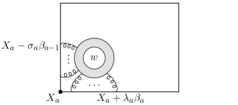
Figure 4: A single-cusp web $W_{a}$, in the sum of Eq. (36).

Generic diagrams for quadrilateral loops are shown in Figs. 4 and 5. In Fig. 4, for example, the $a$th vertex of the polygon represents a cusp vertex that connects two Wilson lines, of velocity $\beta_{a-1}$ and $\beta_{a}$, with $\beta_{0}\equiv\beta_{4}$.

Exponentiation in coordinate space implies that the logarithm of a polygon $P$ is a sum of the web configurations illustrated by the figures,

$$\ln P = \sum_{{\rm cusps}\ a}W_{a}\ +\sum_{{\rm sides}\ \{a+1,a\}}W_{a+1,a}\ +\ W_{\rm plane}\,.$$ (36)

The first terms organize webs associated entirely with one of the cusps of the polygon, constructed in terms of the coordinate webs identified above. Because each edge is of finite length, we must now retain the additional gauge-variant terms associated with the end-point contributions ($E_{\rm end}$ above), which are to be combined with gauge-variant end points from webs connecting three or four sides to derive a gauge-invariant result. The cancellation of subdivergences in webs implies that after a sum over diagrams, only the cusp poles and a single, overall collinear singularity survives Drummond:2007aua ; Erdogan:2014gha . There remains a finite contribution from webs that connect all four (or in general more) of the Wilson lines, and these are represented by the final term in (36).

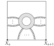
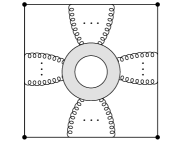
Figure 5: 5 A “side” web $W_{a+1,a}$ in Eq. (36), in this case associated with the lightlike side between $X_{a}$ and $X_{a+1}$. 5 A web that contributes to $W_{\rm plane}$ in Eq. (36).

Evidently, the single-cusp contribution, $W_{a}(\beta_{a},\beta_{a-1})$ has the same gauge-invariant integrand as for the finite Wilson lines in Eq. (10), in terms of the lengths $L_{a}$ of the sides of the polygon, between vertices $a$ and $a+1$

$$W_{a}(\beta_{a},\beta_{a-1},L_{a},L_{a-1})\ =\ \int_{0}^{L_{a}}\!\frac{d\lambda_{a}}{\lambda_{a}}\,\int^{0}_{-L_{a-1}}\!\frac{d\sigma_{a}}{\sigma_{a}}\,w(\alpha_{s}(1/\lambda_{a}\sigma_{a},\varepsilon),\varepsilon)\,.$$ (37)

The web function $w$ for the cusp can depend only on the scalar products of the velocities, and we may assume for simplicity that these are all of the same order.

The two-cusp contributions connect three sides, and the only available singular configuration is when all lines in the web are parallel to the side between the two adjacent vertices. The only invariants on which the web can then depend are of the form $L_{a}\eta$, with $L_{a}$ the length of this side, and $\eta$ a typical distance of vertices in the web from the side. As a result, the general form of the $W_{a+1,a}$ in Eq. (36) is

$$W_{a+1,a}(L_{a})\ =\ \int_{0}^{L_{a}}\frac{d\eta}{\eta}\ w_{a+1,a}\left(\alpha_{s}(\eta L_{a},\varepsilon)\right)\,,$$ (38)

for a function $w_{a+1,a}(\alpha_{s})$, where we assume all the sides are of a similar length. Finally, for the diagrams in which the web is stretched out between more than three sides of a polygon (in this case, the web is connected to all four sides of the quadrilateral), $W_{\rm plane}$, the only scale available is the area of the quadrilateral, and these web contributions are an expansion in the coupling evaluated at the inverse area, with finite coefficients.

The two-loop diagrams for all of these topologies were computed in Drummond:2007aua . We note that in the results quoted there, the cusp anomalous dimension does not appear until all diagrams of the topologies of $W_{a}$ and $W_{a+1,a}$ are combined. Following the prescription for the web integrand given above, however, the two-loop cusp is associated entirely with the diagrams dressing a single corner, $W_{a}$, precisely because the gauge-variant end-point contributions $E_{\rm end}$ of Eq. (24) are not included in that object. For polygons, these gauge-variant terms at two loops, or any order, cancel contributions from the two-cusp contributions $W_{a+1,a}$, which also give rise to gauge-variant terms that cancel those from planar diagrams. These gauge-variant terms contain subdivergences in general. The complete result, of course, is gauge invariant and corresponds at two loops to the full calculation in Refs. Korchemskaya:1992je and Drummond:2007aua .

For polygons, the renormalization group equation has been given in Korchemskaya:1992je ,

$$\frac{d}{d\,\ln\mu^{2}}\ P_{\rm ren}\ =\ -\frac{1}{2}\;\sum_{a}\Gamma_{\rm cusp}(\alpha_{s}(\mu^{2}))\ \ln(\mu^{2}L_{a}L_{a-1}\beta_{a}\cdot\beta_{a-1})\ -\ \Gamma_{\rm co}\left(\alpha_{s}(\mu^{2})\right)\,,$$ (39)

where the $L_{a}$ and $\mu$-dependence of the first term is characteristic of cusps with lightlike Wilson lines Korchemsky:1987wg , and where the second term, $\Gamma_{\rm co}$ was called the collinear anomalous dimension in Ref Korchemskaya:1992je . Aside from overall factors associated with the number of sides of the polygon, the collinear anomalous dimension for the quadrilateral is identical to $G_{\rm eik}$ in Eq. (32), except for the coefficient of $\zeta_{3}$, which differs due to extra diagrams that connect three sides of the quadrilateral.

Polygons of this sort have been studied in the context of a duality to scattering amplitudes in conformal theories Alday:2007hr ; Drummond:2007aua . Here, we consider a four-sided polygon that projects to a square in the $x_{1}/x_{2}$ plane, with side $X$, as in Figs. 4–5. In four dimensions, the loop starts at the origin, travels along the plus-$x_{1}$ direction for a “time” $X^{0}=X$, then changes direction to $x_{2}$ for time $X$, and then moves backwards in time and space, first in the $x_{1}$ direction, then $x_{2}$, back to the origin. We can now use the coordinates $x_{1}$ and $x_{2}$ to define parameters $\lambda_{a}$ and $\sigma_{a}$ for each of the cusp integrals $W_{a}$ in Eq. (37),

$$\begin{array}[]{lcl}\sigma_{1}=-x_{2}\,,&&\lambda_{1}=x_{1}\,,\\ \sigma_{2}=x_{1}-X\,,&&\lambda_{2}=x_{2}\,,\\ \sigma_{3}=x_{2}-X\,,&&\lambda_{3}=X-x_{1}\,,\\ \sigma_{4}=-x_{1}\,,&&\lambda_{4}=X-x_{2}\,.\end{array}$$ (40)

In this notation, we can add the four cusp web integrals of Eq. (37), to get a single integral over $x_{1}$ and $x_{2}$. The web functions, of course, depend on the particular forms of $\lambda$ and $\sigma$ above. We find

$$\sum_{a=1}^{4}W_{a}(\beta_{a},\beta_{a-1})\,=\,\int_{0}^{X}\!\!dx_{1}\int_{0}^{X}\!\!dx_{2}\,\frac{(X-x_{2})[(X-x_{1})w_{1}+x_{1}w_{2}]+x_{2}[x_{1}w_{3}+(X-x_{1})w_{4}]}{x_{1}(X-x_{1})x_{2}(X-x_{2})}\,,$$ (41)

where $w_{a}\equiv w(\alpha_{s}(\lambda_{a}(x_{1},x_{2})\sigma_{a}(x_{1},x_{2})))$. For a conformal theory, all dependence on the $\sigma_{a}$ and $\lambda_{a}$ is in the denominators and we can sum over $a$ to get a result in terms of a constant web function $w_{0}$. Changing variables to $y_{a}=1-2x_{a}/X$, we derive the unregularized form found from the analysis of extremal two-dimensional surfaces embedded in a five-dimensional background in Alday:2007hr ,

$$\sum_{a=1}^{4}W_{a}(\beta_{a},\beta_{a-1})\ =\ \int_{-1}^{1}dy_{1}\,\int_{-1}^{1}dy_{2}\,\frac{4w_{0}}{(1-y_{1}^{2})(1-y_{2}^{2})}\,,$$ (42)

to which we should add the collinear and finite multi-cusp contributions of Fig. 5.

V Conclusions

We have found that when the massless cusp is analyzed in coordinate space, it is naturally written as the exponential of a two-dimensional integral. The integrand, a web function, depends on the single invariant scale through the running of the coupling, which for a theory that is conformal in four dimensions agrees with strong-coupling results Alday:2007hr ; Alday:2008yw ; Kruczenski:2002fb . This agreement extends to aspects of closed, polygonal Wilson loops. These results do not rely on a planar limit 'tHooft:1973jz , but it is natural to conjecture that for large $N_{c}$ the integral may take on an even more direct interpretation in terms of surfaces for nonconformal theories.

In QCD, of course, our explicit knowledge of the web function is limited to the first few terms in the perturbative series, which run out of predictive power as the invariant distance increases. The integral forms derived above, however, hold to all orders in perturbation theory, and may point to an interpolation between short and long distances.

Appendix A Two-loop Integrals

A.1 The 3-scalar integral

To evaluate the the 3-scalar term in Eq. (24), we integrate over the position of the three-gluon vertex after combining the denominators by Feynman parametrization. Introducing the Feynman parameters $\alpha_{1}$ and $\alpha_{2}$, the 3-scalar contribution is given by

$$\begin{split}E_{3s}\ =\ &-\ \mathcal{N}_{3g}(\varepsilon)\int_{0}^{\infty}d\lambda\,d\sigma\int d^{4-2\varepsilon}y\>\frac{\Gamma(3-3\varepsilon)}{\Gamma^{3}(1-\varepsilon)}\\ &\quad\times\int^{1}_{0}d\alpha_{1}\int^{1-\alpha_{1}}_{0}\!\!d\alpha_{2}\frac{(1-\alpha_{1}-\alpha_{2})^{-\varepsilon}\alpha^{-\varepsilon}_{1}\alpha^{-\varepsilon}_{2}}{\left[-y^{2}+2\alpha_{2}(1-\alpha_{1}-\alpha_{2})\lambda\sigma+i\epsilon\right]^{3-3\varepsilon}}\ ,\end{split}$$ (43)

where $y\equiv x-\alpha_{2}\lambda\beta_{1}-(1-\alpha_{1}-\alpha_{2})\sigma\beta_{2}$. The integral over $y$ is straightforward after doing a clockwise Wick rotation,

$$\begin{split}E_{3s}\ =\ &-\ \mathcal{N}_{3g}(\varepsilon)\left(\frac{-i\pi^{2-\varepsilon}}{2^{1-2\varepsilon}}\frac{\Gamma(1-2\varepsilon)}{\Gamma^{3}(1-\varepsilon)}\right)\int_{0}^{\infty}\frac{d\lambda\ d\sigma}{\hskip 11.38109pt(\lambda\sigma)^{1-2\varepsilon}}\\ &\quad\times\int^{1}_{0}d\alpha_{1}\int^{1-\alpha_{1}}_{0}d\alpha_{2}\,(1-\alpha_{1}-\alpha_{2})^{-1+\varepsilon}\,\alpha^{-\varepsilon}_{1}\,\alpha^{-1+\varepsilon}_{2}\ .\end{split}$$ (44)

The integrals over Feynman parameters $\alpha_{1},\alpha_{2}$ now factor from the integrals over eikonal parameters $\lambda,\sigma$. After a change of variables $\eta\equiv\alpha_{2}/(1-\alpha_{1})$, they can be integrated independently,

$$\int^{1}_{0}d\alpha_{1}\,\alpha^{-\varepsilon}_{1}(1-\alpha_{1})^{2\varepsilon-1}\int^{1}_{0}d\eta\,\eta^{\varepsilon-1}(1-\eta)^{\varepsilon-1}\ =\ \frac{1}{\varepsilon^{2}}\Gamma(1-\varepsilon)\Gamma(1+\varepsilon)\ .$$ (45)

In Eq. (44), this gives the scaleless $\lambda,\,\sigma$ integral times a constant with a double pole in $\varepsilon$, given in Eq. (25).

A.2 The end-point term

We now return to the $\lambda_{2}=\Lambda$ end-point contribution from the second term on the right-hand side of Eq. (III.3), which vanishes in the $\Lambda\rightarrow\infty$ limit for any fixed values of the vertex $x^{\mu}$. If we integrate over $x^{\mu}$ first, however, we get a singular contribution, associated with the renormalization of a Wilson line of finite length. It cancels in the gauge-invariant polygons discussed in Sec. IV, and extensively in Refs. Korchemskaya:1992je ; Drummond:2007aua . After the $x^{\mu}$ integral, we have

$$E_{\mbox{\scriptsize end}} \ =\ -\ \mathcal{N}_{3g}(\varepsilon)\left(\frac{-i\pi^{2-\varepsilon}}{2^{1-2\varepsilon}}\frac{\Gamma(1-2\varepsilon)}{\Gamma^{3}(1-\varepsilon)}\right)\int_{0}^{\Sigma}\frac{d\sigma}{\sigma^{1-2\varepsilon}}\int_{0}^{\Lambda}d\lambda$$

$$\quad\times\int^{1}_{0}d\alpha_{1}\int^{1-\alpha_{1}}_{0}\!\!d\alpha_{2}\,\alpha_{1}^{\varepsilon-1}(1-\alpha_{1}-\alpha_{2})^{-\varepsilon}\alpha_{2}^{-\varepsilon}\left[\alpha_{2}\Lambda+(1-\alpha_{1}-\alpha_{2})\lambda\right]^{-1+2\varepsilon}\ .$$

Changing variables to $\eta=\alpha_{2}/(1-\alpha_{1})$, we find a form that is easy to evaluate,

$$E_{\mbox{\scriptsize end}} \ =\ -\ \mathcal{N}_{3g}(\varepsilon)\left(\frac{-i\pi^{2-\varepsilon}}{2^{1-2\varepsilon}}\frac{\Gamma(1-2\varepsilon)}{\Gamma^{3}(1-\varepsilon)}\right)\int_{0}^{\Sigma}\frac{d\sigma}{\sigma^{1-2\varepsilon}}$$

$$\hskip 14.22636pt\times\ \int^{1}_{0}d\alpha_{1}\,\alpha_{1}^{\varepsilon-1}\int^{1}_{0}\!\!d\eta\,(1-\eta)^{-\varepsilon}\eta^{-\varepsilon}\ \int_{0}^{\Lambda}\ d\lambda\left[\eta\Lambda+(1-\eta)\lambda\right]^{-1+2\varepsilon}$$

$$\ =\ \left(\frac{\alpha_{s}}{\pi}\right)^{2}\ C_{A}C_{F}\ \left(2\pi\mu^{2}\Lambda\Sigma\right)^{2\varepsilon}\ \frac{1}{64\varepsilon^{4}}\ \left[\Gamma(1-2\varepsilon)\,\Gamma(1-\varepsilon)\,\Gamma(1+\varepsilon)\ -\ \Gamma^{2}(1-\varepsilon)\right]\,.$$

If we add this result to the expressions found by integrating the $\sigma$ and $\lambda$ integrals of $E_{3s}$, Eq. (25) and $E_{pse}$, Eq. (26), over the finite intervals of $0$ to $\Sigma$ and $\Lambda$, we recover the expression quoted for this diagram in Refs. Korchemskaya:1992je ; Drummond:2007aua .