Exploiting boundary states of imperfect spin chains for high-fidelity state transfer

Abstract

We study transfer of a quantum state through $XX$ spin chains with static imperfections. We combine the two standard approaches for state transfer based on (i) modulated couplings between neighboring spins throughout the spin chain and (ii) weak coupling of the outermost spins to an unmodulated spin chain. The combined approach allows us to design spin chains with modulated couplings and localized boundary states, permitting high-fidelity state transfer in the presence of random static imperfections of the couplings. The modulated couplings are explicitly obtained from an exact algorithm using the close relation between tridiagonal matrices and orthogonal polynomials [Linear Algebr. Appl. 21, 245 (1978)]. The implemented algorithm and a graphical user interface for constructing spin chains with boundary states (spinGUIn) are provided as Supplemental Material.

I Introduction

Spin chains have attracted much attention in recent years (for reviews see Bose (2007); Kay (2010)) because of their ability either to act as quantum communication channels Bose (2003); Christandl et al. (2004); Wójcik et al. (2005) or to generate highly entangled states for quantum computation Yung and Bose (2005); Clark et al. (2005, 2007). The use of spin chains for both of these tasks has been considered in the context of various physical systems: Implementations of spin chains may connect nitrogen-vacancy registers in diamond Yao et al. (2011) or entangle internal states of an array of ultracold atoms confined to an optical lattice Clark et al. (2005). Arrays of capacitively coupled flux qubits have also been shown to be suited for quantum state transfer Lyakhov and Bruder (2005).

In particular, spin chains of $XX$ type Lieb et al. (1961) can be used as a quantum channel, i.e., a quantum state (qubit) placed at one end of the chain can be perfectly transferred to the other end as a result of the coherent time evolution. Two different strategies have been suggested to achieve perfect state transfer (PST) in this context. The first approach relies on modulated couplings between neighboring spins throughout the spin chain Christandl et al. (2004); Yung and Bose (2005). More precisely, the quality of the state transfer depends on the energy spectrum of the spin chain and suitable couplings for PST are obtained by solving an inverse eigenvalue problem (IEP). The prototypical couplings between spins for PST correspond to a linear spectrum Christandl et al. (2004), also considered relevant to the dynamics of electrons in $N$-level systems Eberly et al. (1977); Białynicka-Birula et al. (1977); Cook and Shore (1979); Shore and Cook (1979).

The second approach is based on weak couplings of the outermost spins to the rest of the otherwise unmodulated spin chain Wójcik et al. (2005, 2007); Zwick et al. (2012). In this weak-coupling limit the dynamics of the spin chain reduces to an effective two- or three-level system consisting of states localized at the boundaries of the spin chain (boundary states) and state transfer is a consequence of Rabi-type oscillations Shore and Cook (1979); Wójcik et al. (2007). PST is only achieved in the limit of vanishing couplings of the outermost spins of the chain. The advantage of this approach is that transfer does not depend on details of the spin chain, i.e., no modulation of inner spin couplings is required.

The primary aim of this paper is to combine these two strategies. We construct spin chains with modulated couplings; however, these are chosen such that state transfer takes place mainly through boundary states. The resulting spin chains therefore have two qualities: they permit PST through a perfectly engineered chain, and their dynamics, involving only a few states, is robust to small variations of the spin couplings. To construct these spin chains we start from the energy spectrum and add nearly zero eigenvalues, which under specific conditions entails boundary states.

The couplings of the spin chains are explicitly obtained by solving the IEP with a numerically stable algorithm developed by de Boor and Golub de Boor and Golub (1978). We describe the algorithm adapted to the specific problem of PST through spin chains and provide its implementation as matlab code. In addition, we supply a graphical user interface for designing spin chains with boundary states, called spinGUIn, as Supplemental Material sup .

As a proof of principle, we compare transfer fidelities of different spin chains with static imperfections of the spin couplings, similar to the analysis in Refs. De Chiara et al. (2005); Zwick et al. (2011, 2012). The imperfections are modeled as relative fluctuations of the couplings drawn from a uniform distribution. The resulting distributions of the transfer fidelities reveal that chains with boundary states are more resilient to imperfections. This is reflected in more instances of high-fidelity transfer through the spin chain.

The structure of this article is as follows: In Sec. II we recall the basics of state transfer through spin chains. In Secs. III and IV we give necessary details of the two strategies for achieving state transfer using modulated couplings and weakly coupled end spins. Furthermore, we describe the algorithm by de Boor and Golub, which may be applied to the modulated coupling strategy. In Sec. V we present the combined approach and apply it to specific examples, including an analysis of their transfer fidelity in the presence of imperfect couplings. We end with the conclusions in Sec. VI.

II State transfer

To start with, we recall the basics of state transfer through a one-dimensional $XX$ spin chain with the Hamiltonian

$$\hat{H}_{S}=\frac{1}{2}\sum_{j=1}^{N-1}b_{j}\left(\hat{\sigma}^{x}_{j}\hat{\sigma}^{x}_{j+1}+\hat{\sigma}^{y}_{j+1}\hat{\sigma}^{y}_{j}\right)+\frac{1}{2}\sum_{j=1}^{N}a_{j}\left(\mathbb{1}+\hat{\sigma}^{z}_{j}\right)\,.$$

Here, $b_{j}$ are the spatially dependent spin couplings between neighboring sites, $a_{j}$ are local external fields, and $\hat{\sigma}^{x},\hat{\sigma}^{y},\hat{\sigma}^{z}$ are the Pauli matrices. It is convenient to map the spin Hamiltonian $\hat{H}_{S}$ to a one-dimensional fermionic hopping model using the Jordan-Wigner transformation Lieb et al. (1961), which yields the equivalent Hamiltonian

$$\hat{H}_{F}=\sum_{j=1}^{N-1}b_{j}\left(\hat{c}^{\dagger}_{j}\hat{c}_{j+1}+\hat{c}^{\dagger}_{j+1}\hat{c}_{j}\right)+\sum_{j=1}^{N}a_{j}\hat{c}^{\dagger}_{j}\hat{c}_{j}\,.$$

The operators $\hat{c}^{\dagger}_{j}$ ($\hat{c}_{j}$) create (annihilate) a fermion at site $j$ and obey the usual anticommutation relations. Since the Hamiltonian $\hat{H}_{F}$ commutes with the total number operator $\hat{n}=\sum_{j=1}^{N}\hat{c}^{\dagger}_{j}\hat{c}_{j}$, the Hilbert space can be decomposed into subspaces $\mathcal{H}_{n}$ corresponding to different total fermion numbers $n$. For transferring a single qubit we restrict our considerations to the subspace $\mathcal{H}_{0}\oplus\mathcal{H}_{1}$. The subspaces $\mathcal{H}_{0}$ and $\mathcal{H}_{1}$ are spanned by the vacuum state $|\mathrm{vac}\rangle$ and the single-fermion Fock states $|j\rangle=\hat{c}^{\dagger}_{j}|\mathrm{vac}\rangle$, respectively.

For state transfer the spin chain is initialized in the vacuum state. The qubit is written into the first spin of the chain at time $t=0$, so that the state of the spin chain is $|\psi(0)\rangle=c_{0}|\mathrm{vac}\rangle+c_{1}|1\rangle$. Subsequently, the qubit is transferred under the coherent evolution $\hat{U}(t)=\mathrm{e}^{-\mathrm{i}\hat{H}_{F}t}$ to the spin at site $N$ after the transfer time $t=\tau$, where it can be read out. In the ideal case we have $|\psi(\tau)\rangle=\hat{U}(\tau)|\psi(0)\rangle=c_{0}|\mathrm{vac}\rangle+c_{1}|N\rangle$, i.e., PST is achieved. The unitary operator $\hat{U}(\tau)$ and therefore the Hamiltonian $\hat{H}_{F}$ have to fulfill certain conditions to ensure PST. Since the vacuum state has a trivial time evolution, the conditions only apply to the Hamiltonian for the subspace $\mathcal{H}_{1}$, which in the single-fermion basis $\{|j\rangle\}$ is given by the tridiagonal matrix

$$H_{N}=\left(\begin{array}[]{ccccc}a_{1}&b_{1}&0&\cdots&0\\ b_{1}&a_{2}&b_{2}&\cdots&0\\ 0&b_{2}&a_{3}&\cdots&0\\ \vdots&\vdots&\vdots&\ddots&b_{N-1}\\ 0&0&0&b_{N-1}&a_{N}\end{array}\right)\,.$$

III Modulated couplings

The approach based on modulated couplings between neighboring spins relies on two conditions of $H_{N}$ (for details see Yung and Bose (2005)). First, the matrix $H_{N}$ has to be symmetric along the antidiagonal, i.e., the entries of $H_{N}$ fulfill the condition $a_{N-j+1}=a_{j}$ and $b_{N-j}=b_{j}$. The matrix $H_{N}$, being symmetric along the antidiagonal, is said to be persymmetric. As a result of the reflection symmetry, the eigenvectors $|\lambda_{k}\rangle$ of the matrix $H_{N}$ have definite parities. Moreover, if the eigenvalues $\lambda_{k}$ are in increasing order then the eigenvectors $|\lambda_{k}\rangle$ change parity alternatively, i.e., the mirror-inverted eigenstates $|{\overline{\lambda}}_{k}\rangle$ satisfy the relation $|{\overline{\lambda}}_{k}\rangle=(-1)^{k}|\lambda_{k}\rangle$ upon assuming that even (odd) $k$ label even (odd) eigenstates $|\lambda_{k}\rangle$.

Second, for PST the eigenvalues $\lambda_{k}$ have to fulfill the condition

$$\mathrm{e}^{-\mathrm{i}\lambda_{k}\tau}=(-1)^{k}\mathrm{e}^{\mathrm{i}\Phi}$$ (1)

for a constant transfer time $\tau$ and phase $\Phi$. In fact, if the initial single-fermion state $|\varphi(0)\rangle\in\mathcal{H}_{1}$ is expanded in terms of eigenvectors as $|\varphi(0)\rangle=\sum_{k}c_{k}|\lambda_{k}\rangle$ with constant coefficients $c_{k}$, then the state at time $\tau$ is given by $|\varphi(\tau)\rangle=\sum_{k}c_{k}\mathrm{e}^{-\mathrm{i}\lambda_{k}\tau}|\lambda_{k}\rangle$. On the other hand, since $|\varphi(\tau)\rangle$ is the mirror-inverted state of $|\varphi(0)\rangle$, by assumption we have $|\varphi(\tau)\rangle=\mathrm{e}^{\mathrm{i}\Phi}\sum_{k}c_{k}|\overline{\lambda}_{k}\rangle=\mathrm{e}^{\mathrm{i}\Phi}\sum_{k}c_{k}(-1)^{k}|\lambda_{k}\rangle$. A comparison between the two expressions for $|\varphi(\tau)\rangle$ then indeed yields the condition in Eq. (1). The generalization by global phase factor $\mathrm{e}^{\mathrm{i}\Phi}$ can be made since the phase $\Phi$ can be compensated for, e.g., by applying a constant external field $a_{j}=-\Phi/\tau$ for all $j$.

Thus, finding the Hamiltonian $H_{N}$ for PST reduces to an IEP, namely, calculating the couplings $a_{j}$ and $b_{j}$ for a given sequence of eigenvalues $\lambda_{k}$ that fulfill the condition in Eq. (1) for a fixed $\tau$. A convenient choice is to set the transfer time $\tau$ to the fixed value $\pi$ so that the eigenenergies $\lambda_{k}$ take integer values. Other transfer times are obtained by rescaling the spectrum by an overall energy scale.

Solving the IEP

We now describe the algorithm developed by de Boor and Golub de Boor and Golub (1978) for solving the IEP in the case where $H_{N}$ is persymmetric and all eigenvalues $\lambda_{k}$ are distinct. Solving the IEP based on continued fractions has been suggested recently in Ref. Wang et al. (2011) for achieving PST, and similarly in the context of electric circuit theory Sussman-Fort (1982). We chose the algorithm by de Boor and Golub, which was in part motivated by Ref. Hochstadt (1974), because of its clarity and straightforward numerical implementation.

We start with basic definitions related to orthogonal polynomials and tridiagonal matrices. We denote by $H_{j}$ the left principal submatrix, which is formed by deleting the last $N-j$ rows and columns of $H_{N}$. Further, we introduce the polynomials $p_{j}(x)=\det(x-H_{j})$, with $j=1,\ldots,N$, and define $p_{0}=1$ and $p_{-1}=0$. Clearly $p_{j}(x)$ are the characteristic polynomials of the matrices $H_{j}$, and in particular, $p_{N}(\lambda_{k})=0$ for the eigenvalues $\lambda_{k}$. It then follows directly from Laplace’s formula for the expansion of determinants that the polynomials $p_{j}(x)$ satisfy the three-term recursion relation

$$p_{j}=(x-a_{j})p_{j-1}-b^{2}_{j-1}p_{j-2}\,.$$ (2)

Next we introduce the discrete scalar product $\langle\;,\>\rangle$ defined as

$$\langle f,g\rangle=\sum_{k}w_{k}\,f(\lambda_{k})g(\lambda_{k})$$ (3)

for any polynomials $f$ and $g$ up to degree $N$. As shown in Ref. de Boor and Golub (1978), the polynomials $p_{j}$ are orthogonal with respect to the scalar product in Eq. (3), i.e., $\langle p_{i},p_{j}\rangle=0$ for $i\neq j$, provided that the spectrum-dependent weights are defined by $w_{k}=\left|\mathrm{d}p_{N}(x)/\mathrm{d}x\right|^{-1}$ evaluated at $x=\lambda_{k}$. Using the expression $p_{N}(x)=\prod_{k}(x-\lambda_{k})$ for the characteristic polynomial, one finds the explicit form for the weights:

$$w_{k}=\bigg{|}\prod_{p\neq k}(\lambda_{k}-\lambda_{p})\bigg{|}^{-1}\,.$$ (4)

The orthogonality of the polynomials $p_{j}$ and the recurrence relation make it possible to express the coefficients $a_{j}$ and $b_{j}$ solely in terms of $p_{j}$ and $p_{j-1}$. By taking the scalar product with $p_{j-1}$ on both sides of Eq. (2) one obtains

$$a_{j}=\frac{\langle xp_{j-1},p_{j-1}\rangle}{\langle p_{j-1},p_{j-1}\rangle}\,.$$ (5)

Similarly, taking the scalar product with $p_{j-2}$ and $p_{j}$ on both sides of Eq. (2) yields $b_{j-1}^{2}\langle p_{j-2},p_{j-2}\rangle=\langle xp_{j-1},p_{j-2}\rangle$ and $\langle p_{j},p_{j}\rangle=\langle p_{j},xp_{j-1}\rangle$, respectively. Hence using the property of the scalar product $\langle xf,g\rangle=\langle f,xg\rangle$, one finds

$$b_{j}=\frac{||p_{j}||}{||p_{j-1}||}$$ (6)

with the norm $||f||=\sqrt{\langle f,f\rangle}$.

The algorithm is based on the key observation that the polynomials $p_{j}$ and coefficients $a_{j}$ and $b_{j}$ can be determined recursively starting with the polynomials $p_{-1}=0$ and $p_{0}=1$. The required weights $w_{k}$, which specify scalar product in Eq. (3), are readily calculated from the eigenvalues $\lambda_{k}$. Thus the algorithm for solving the IEP consists of the following steps:

1. Calculate the weights $w_{k}$ for the given $\lambda_{k}$ from Eq. (4). Subsequently repeat steps 2–4 for increasing $j$ starting with $j=1$.

2. Calculate the coefficient $a_{j}$ from Eq. (5).

3. Find the values of $p_{j}(x)$ at $x=\lambda_{k}$ from Eq. (2).

4. Calculate the coefficient $b_{j}$ from Eq. (6).

For odd $N$ the steps have to be repeated up to $j=(N+1)/2$ and for even $N$ up to $j=N/2$.

As noted by de Boor and Golub, the algorithm provides a stable means of computing the entries of $H_{N}$. However, the maximum length of the spin chain $N$ is limited by floating point under- or overflow in the weights or the values of the polynomials. To ameliorate this problem during execution of the algorithm it is advisable to scale the spectrum $\{\lambda_{k}\}$ into the interval $[-1,1]$ with appropriate rescaling of the resulting coefficients $a_{j}$ and $b_{j}$. This prevents the weights $w_{k}\sim 1/\Delta\lambda^{N-1}$ ($\Delta\lambda$ being the typical difference between any two of the $\lambda_{k}$) from becoming smaller than the typical floating point precision. Moreover, the polynomial terms $p_{j}(\lambda_{k})$ in the calculation are potentially large without scaling since they take values of the order of $\lambda_{k}^{(N+1)/2}$ for $j=(N+1)/2$. With this proviso the algorithm yields accurate results for spin chains with lengths up to a few hundred spins, as found by testing against the exact solutions for the linear and cosine spectrum (defined in Sec. V).

Note that the algorithm does not involve approximations and can be used to obtain exact analytic results for the coefficients $a_{j}$ and $b_{j}$. For instance, a useful analytic result following from Eq. (5) and based on symmetry arguments is that all $a_{j}$ vanish if the eigenvalues $\lambda_{k}$ are symmetrically distributed around zero (cf. Lemma 5 in Kay (2010)); the converse is also true Shore and Cook (1979).

IV Weakly coupled end spins

The second approach relies on weak couplings of the outermost spins (end spins) to the rest of the chain, i.e., the couplings $b_{1}$ and $b_{N-1}$ are considerably smaller than the otherwise arbitrary spin couplings $b_{j}$ with $j=2,\ldots,N-2$. To analyze this type of spin chain we can therefore use perturbation theory in the couplings $b_{1}$, $b_{N}$. Accordingly, we partition the Hamiltonian into two parts $H_{N}=H_{0}+V$ with

$$V=\left(\BMAT(rc){cc}{cc}\BMAT(rc){ccc}{ccc}0&b_{1}\\ b_{1}0\\ &\mbox{\huge 0}\\ \mbox{\huge 0}\BMAT(rc){ccc}{ccc}\\ 0b_{N-1}\\ b_{N-1}0\right)$$

and $H_{0}=H_{N}-V$, where for simplicity we assumed that the local external fields $a_{j}$ vanish.

As customary, we introduce the eigenvalues $\xi_{k}$ and eigenstates $|\xi_{k}\rangle$ of $H_{0}$, i.e., $H_{0}|\xi_{k}\rangle=\xi_{k}|\xi_{k}\rangle$. Before applying perturbation theory we make the following observations: First, the eigenvalues $\xi_{k}$ of $H_{0}$ are symmetrically distributed around zero. Therefore, if the number of spins $N$ is odd then the Hamiltonian $H_{0}$ has an eigenstate $|\xi_{0}\rangle$ with $\xi_{0}=0$, i.e., a zero mode. This mode has the property that all odd components in the position basis $\{|j\rangle\}$ vanish identically and that the even components have alternating signs. Second, $H_{0}$ has two additional zero modes regardless of $N$ which are localized at sites $1$ and $N$, i.e., the two boundary states $|\xi_{1}\rangle\equiv|1\rangle$ and $|\xi_{N}\rangle\equiv|N\rangle$ are zero modes of $H_{0}$. In sum, the $\xi_{k}=0$ subspace is spanned by the states $|\xi_{0}\rangle,|\xi_{1}\rangle,|\xi_{N}\rangle$ for odd $N$ and by the states $|\xi_{1}\rangle,|\xi_{N}\rangle$ for even $N$.

We determine the evolution of the state $|\varphi(t)\rangle$ initially in state $|\xi_{1}\rangle\equiv|1\rangle$ by using time-dependent perturbation theory Langhoff et al. (1972). To this end $|\varphi(t)\rangle$ is expanded in the basis $\{|\xi_{k}\rangle\}$ as

$$|\varphi(t)\rangle=\sum_{k}c_{k}(t)\,\mathrm{e}^{-\mathrm{i}\xi_{k}t}|\xi_{k}\rangle$$

where $c_{k}(t)$ are time-dependent coefficients with initial conditions $c_{k}(0)=\delta_{1k}$. Inserting $|\varphi(t)\rangle$ into the Schrödinger equation yields

$$\mathrm{i}\frac{\partial}{\partial t}c_{p}(t)=\sum_{k}V_{pk}\,c_{k}(t)\,\mathrm{e}^{-\mathrm{i}(\xi_{k}-\xi_{p})t}$$

with the matrix elements $V_{pk}=\langle\xi_{p}|V|\xi_{k}\rangle$. The coupled equations for the $c_{k}(t)$ can be solved approximately by separation of time scales Shore and Cook (1979). As a first step, the equations for the coefficient $c_{k}(t)$ with $k\neq 0,1,N$ are solved under the approximation that the slowly varying $c_{0}(t)$, $c_{1}(t)$ and $c_{N}(t)$ are constant, which yields $c_{k}(t)\approx(1-\mathrm{e}^{\mathrm{i}\xi_{k}t})[V_{k1}c_{1}(t)+V_{kN}c_{N}(t)]/\xi_{k}$. After inserting these approximate solutions into the equations for $c_{0}(t)$, $c_{1}(t)$, $c_{N}(t)$ and neglecting all fast oscillating terms $\mathrm{e}^{-\mathrm{i}\xi_{k}t}$ we obtain

$$\mathrm{i}\frac{\partial}{\partial t}\left(\begin{array}[]{c}c_{1}\\ c_{0}\\ c_{N}\\ \end{array}\right)\approx\left(\begin{array}[]{ccc}\Delta_{1}&V_{10}&\frac{1}{2}\Omega\\ V_{01}&0&V_{0N}\\ \frac{1}{2}\Omega&V_{N0}&\Delta_{N}\\ \end{array}\right)\left(\begin{array}[]{c}c_{1}\\ c_{0}\\ c_{N}\\ \end{array}\right)\,,$$ (7)

where the detunings $\Delta_{i}$ and the frequency $\Omega$ are given by

$$\Delta_{i}=-\sum_{k}\frac{|V_{i0}|^{2}}{\xi_{k}}\qquad\Omega=-2\sum_{k}\frac{V_{1k}V_{kN}}{\xi_{k}^{2}}\,.$$

Because of the symmetry of the problem the detunings $\Delta_{i}$ vanish identically Shore and Cook (1979). We discuss the dynamics of the state $|\varphi(t)\rangle$ resulting from Eq. (7) for the case $V_{01}=V_{0N}=\nu/\sqrt{2}$ and $b_{1}=b_{N-1}=b$.

If $N$ is odd then the system has a zero mode $|\xi_{0}\rangle$ and the dominant contributions in the limit of weak couplings $b\rightarrow 0$ come from the matrix elements $\nu\sim b$ since the second-order frequencies scale as $\Omega\sim b^{2}$. The state evolves according to

$$|\varphi(t)\rangle=\cos^{2}\left(\frac{\nu t}{2}\right)|1\rangle-\frac{\mathrm{i}\sin(\nu t)}{\sqrt{2}}|\xi_{0}\rangle-\sin^{2}\left(\frac{\nu t}{2}\right)|N\rangle$$

and thus is transferred from site $1$ to $N$ after the time $\tau=\pi/\nu\sim 1/b$. The (unnormalized) eigenstates of the matrix in Eq. (7) are given by $|1\rangle-|N\rangle$ and $|1\rangle\pm|\xi_{0}\rangle+|N\rangle$ with eigenvalues $0$ and $\pm\nu$, respectively. Thus the perturbation $V$ leads to strong mixing of the boundary states $|1\rangle$, $|N\rangle$ with the zero mode $|\xi_{0}\rangle$ and lifts their degeneracy with an energy splitting proportional to $b$.

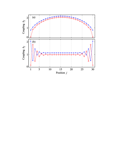
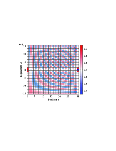
Figure 1: (Color online) Couplings $b_{j}$ between neighboring spins for perfect state transfer before (full dots $\bullet$) and after (empty dots $\circ$) adding boundary states to the spin chain. (a) The outermost couplings $b_{1}$, $b_{N}$ of the spin chain with linear spectrum are reduced when boundary states are added. (b) The couplings of the spin chain with inverted quadratic spectrum are approximately mirrored along the horizontal axis. (c) Components of the eigenstates $|\lambda_{k}\rangle$ in the position basis $\{|j\rangle\}$ corresponding to the modified couplings in (b). The boundary states $|\lambda_{-1}\rangle$, $|\lambda_{0}\rangle$ and $|\lambda_{1}\rangle$ can be clearly seen. The parameters are set to $N=31$, $A=7$ and the $b_{j}$ are scaled by $1/25$ and $1/100$ in (a) and (b), respectively.

If $N$ is even then the zero mode $|\xi_{0}\rangle$ is absent and Eq. (7) describes on-resonance Rabi oscillations between the states $|1\rangle$ and $|N\rangle$ at the Rabi frequency $\Omega$. Accordingly we have

$$|\varphi(t)\rangle=\cos\left(\frac{\Omega t}{2}\right)|1\rangle-\mathrm{i}\sin\left(\frac{\Omega t}{2}\right)|N\rangle$$

and state transfer takes place after the time $\tau=\pi/\Omega\sim 1/b^{2}$. The eigenstates under the effect of the perturbation $V$ are $|1\rangle\pm|N\rangle$ with eigenvalues $\pm\Omega$, and thus we have an energy splitting proportional to $b^{2}$.

The perturbative approach is valid provided that $\nu,\Omega\ll\xi_{\mathrm{min}}$, where $\xi_{\mathrm{min}}$ is the non-zero eigenvalue with the smallest magnitude. In this regime the contributions from high-frequency modes with $\xi_{k}\geq\xi_{\mathrm{min}}$ average out on the time scale of the state transfer. In particular, PST is achieved only in the limit of vanishing couplings $b_{1}$ and $b_{N-1}$, which is the main drawback of this approach. On the other hand, in this limit PST is possible for arbitrary configurations of the inner couplings $b_{j}$ with $j=2,\ldots,N-2$.

V Combined approach

We combine the two approaches in order to endow modulated spin chains with boundary states. State transfer then takes place mainly through the boundary states, making it more robust to imperfections, and yet is perfect even for finite couplings to the end spins. As seen previously, nearly zero eigenvalues in the spectrum of the spin chain, i.e., eigenvalues significantly smaller in magnitude than any other eigenvalue, are a signature of boundary states. The crucial question is if the converse is also true, i.e., if adding nearly zero eigenvalues is sufficient to introduce boundary states. The answer is no—the presence or absence of boundary states depends on the entire spectrum of the chain.

In order to show this we focus on spin chains with odd $N$; however, the arguments are similar for even $N$. The condition for state transfer through boundary states is $\nu\ll\xi_{\mathrm{min}}$, or equivalently $b\ll\xi_{\mathrm{min}}$. To obtain a condition only on the spectrum we make two observations: First, we find from the algorithm by de Boor and Golub that $b^{2}=\sum_{k}w_{k}\lambda_{k}^{2}/\sum_{k}w_{k}$, which is the weighted variance of the spectrum. Second, we notice that $\xi_{\mathrm{min}}$ is identical to $\lambda_{\mathrm{min}}$ provided nearly zero eigenvalues are excluded from the minimum. Therefore the condition for state transfer through boundary states in terms of the eigenvalues $\lambda_{k}$ and the weights $w_{k}=|\prod_{p\neq k}(\lambda_{k}-\lambda_{p})|^{-1}$ reads

$$\frac{\sum_{k}w_{k}\lambda_{k}^{2}}{\sum_{k}w_{k}}\ll\lambda^{2}_{\mathrm{min}}\,.$$ (8)

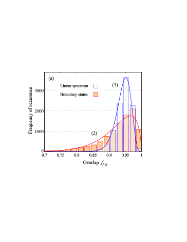
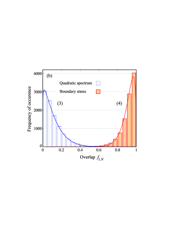
Figure 2: (Color online) The histogram and best-fit $\beta$ distribution of the overlap $f_{1,N}$ for the same spin chains as in Fig. 1 with randomly perturbed couplings $b_{j}$. (a) Adding boundary states to the chain with linear spectrum results in more instances of high-fidelity transport and a broader distribution of $f_{1,N}$. (b) The average transport fidelity of the chain with inverted quadratic spectrum is significantly improved by adding boundary states. The best-fit $\beta$ distribution corresponding to the curves labeled (1)–(4) yields $\alpha=\{96.7,19.3,1.11,15.6\}$, $\beta=\{5.88,1.63,8.65,1.48\}$ and the average $\mu=\{0.943,0.922,0.114,0.914\}$.

Even though Eq. (8) is the desired result we gain more insight by discussing it on the basis of a stepwise linear spectrum. The specific spectrum consist of three bands separated by gaps $\Gamma$, taking the role of $\lambda_{\mathrm{min}}$. The $m$ nearly zero eigenvalues in the central band and the $M$ eigenvalues in each of the peripheral bands have inter-level spacing $\delta$ and $\Delta$, respectively. We estimate the values of the weights $w_{k}$ to determine the regime of $\delta$, $\Gamma$, $\Delta$ for which Eq. (8) is fulfilled. Noting that the weights $w_{k}$ depend on the distance between the eigenvalues we find the scalings

$$w_{k}^{\mathrm{cen}}\sim\frac{1}{\delta^{m}\Gamma^{2M}}\,,\qquad w_{k}^{\mathrm{per}}\sim\frac{1}{\Delta^{M}\Gamma^{m}(2\Gamma)^{M}}\,,$$

where $w_{k}^{\mathrm{cen}}$ and $w_{k}^{\mathrm{per}}$ are the typical weights for the eigenvalues $\lambda_{k}$ located in the central and the peripheral bands, respectively. Now, Eq. (8) is fulfilled if contributions from large eigenvalues in the peripheral bands to the weighted variance are small, i.e., $w_{k}^{\mathrm{per}}\ll w_{k}^{\mathrm{cen}}$, or equivalently

$$\left(\frac{\delta}{\Gamma}\right)^{m}\left(\frac{\Gamma}{\Delta}\right)^{M}\ll 1\,.$$

Thus, eigenvalues in the central band lead to boundary states of the spin chain in the regime $\delta\ll\Gamma$ and $\Delta\sim\Gamma$.

To illustrate the combined approach we consider two examples, namely, the linear spectrum and an inverted quadratic spectrum. Nearly zero eigenvalues are introduced by changing the original spectrum $\lambda_{k}$ to the shifted spectrum $\tilde{\lambda}_{k}=\lambda_{k}-\mathrm{sgn}(\lambda_{k})C$, where $C<\lambda_{\mathrm{min}}$ is a constant. This shifting procedure is applicable to all spectra and leaves the length of the spin chain unchanged.

The linear spectrum is given by $\lambda_{k}=Ak$, where the index $k$ runs from $-\frac{1}{2}(N-1)$ to $\frac{1}{2}(N-1)$, and $A\gg 1$ is an arbitrary odd integer so that $\tau=\pi/A$. After shifting with $C=A-1$ the spectrum contains two eigenvalues $\tilde{\lambda}_{\pm 1}=\pm 1$ with boundary states $|\tilde{\lambda}_{\pm 1}\rangle$. Of the corresponding couplings only $b_{1}$, $b_{N-1}$ are significantly reduced, as shown in Fig. 1(a). Both spin chains, with spectrum $\lambda_{k}$ and $\tilde{\lambda}_{k}$, support PST and their transfer times are related by $\tilde{\tau}=A\tau$.

The inverted quadratic spectrum is defined by $\lambda_{k}=k(N-1-|k|)$. The corresponding couplings $b_{j}$ strongly oscillate toward the end of the chain and are approximately constant in the center. The shifted spectrum with $C=N-3$ has two eigenvalues $\tilde{\lambda}_{\pm 1}=\pm 1$ with boundary states $|\tilde{\lambda}_{\pm 1}\rangle$. Both spin chains, with spectrum $\lambda_{k}$ and $\tilde{\lambda}_{k}$, support PST with identical transfer times. The couplings $b_{j}$ and the eigenstates $|\lambda_{k}\rangle$ are shown in Figs. 1(b) and 1(c), respectively.

As an aside, spin chains with cosine spectrum $\lambda_{k}=2\cos\left[\pi k/(N+1)\right]$ and constant couplings $b_{j}=1$ do not support PST but can still be endowed with boundary states. The shifting procedure significantly reduces the outermost couplings $b_{1}$, $b_{N-1}$ and leads to slight oscillations of the inner couplings. This represents an alternative to the modification of the cosine spectrum suggested in Ref. Karbach and Stolze (2005) in order to achieve PST.

Random static imperfections

We now turn to the performance of spin chains in the presence of static imperfections in the couplings and show that boundary states improve the transfer fidelity. For this purpose we numerically evaluate the transfer fidelity of spin chains with randomized couplings $b^{\mathrm{rnd}}_{j}=b_{j}(1+R)$, where $R$ is a uniformly distributed random variable in the interval $[-r,r]$. We use the overlap $f_{1,N}(\tau)=|\langle N|\mathrm{e}^{-\mathrm{i}H_{N}\tau}|1\rangle|$, taking values in the interval $[0,1]$, to assess the performances of the chain. The overlap $f_{1,N}$ is related to the transfer fidelity $F$ of the state transfer averaged over all input states on the Bloch sphere by $F=\frac{1}{2}+\frac{1}{3}f_{1,N}+\frac{1}{6}f_{1,N}^{2}$ Bose (2007). The transfer time $\tau$ is fixed to the value of the perfectly engineered chain ($r=0$), in which case $f_{1,N}(\tau)=1$.

We reconsider the spin chains with linear and inverted quadratic spectrum and compare the distribution of the overlap $f_{1,N}(\tau)$ with and without boundary states, sampled over $10^{4}$ transfers. In addition, we fit a $\beta$ distribution to the numerically obtained distribution of $f_{1,N}(\tau)$. The $\beta$ distribution is defined on the interval $(0,1)$ by the probability density $P(x)=[B(\alpha,\beta)]^{-1}\,x^{\alpha-1}(1-x)^{\beta-1}$, where $\alpha$ and $\beta$ are two positive shape parameters and $B(\alpha,\beta)=\int_{0}^{1}\mathrm{d}t\,t^{\alpha-1}(1-t)^{\beta-1}$ is the $\beta$ function. The average value is given by $\mu=\alpha/(\alpha+\beta)$ and the variance by $\sigma^{2}=\alpha\beta/[(\alpha+\beta)^{2}(\alpha+\beta+1)]$.

Figure 2 shows the distribution of the $f_{1,N}(\tau)$ for the linear and inverted quadratic spectrum, as well as their shifted counterpart with boundary states. In all cases the randomized couplings (at the level $r=0.05$) result in reduced transfer fidelities. Both spin chains with linear spectrum are remarkably resilient to imperfections; however, the corresponding distributions of the overlap $f_{1,N}(\tau)$ differ noticeably, as shown in Fig. 2(a). Boundary states lead to a broader distribution of $f_{1,N}(\tau)$ and to substantially more instances of high-fidelity state transfer. Spin chains with boundary states are therefore advantageous in a scenario where varying couplings are caused by imperfect fabrication (or tuning) and only high-quality chains, say with $f_{1,N}(\tau)\geq 0.98$, are selected. Note that the performance of the spin chain with a linear spectrum can be further improved by increasing the parameter $A$.

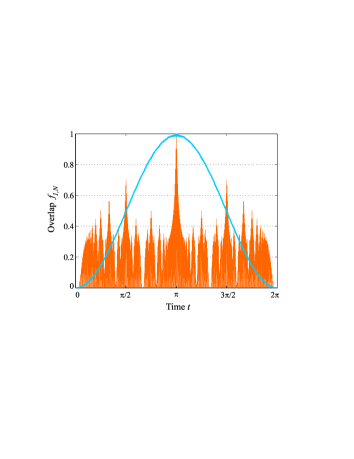
Figure 3: (Color online) The overlap $f_{1,N}$ as a function of time $t$ for the spin chains with the inverted quadratic spectrum of Fig. 1(b). The irregular time dependence of $f_{1,N}$ (orange peaks) with high-frequency oscillations and a sharp peak at $t=\pi$ is smoothed out by adding boundary states, resulting in a regular sine dependence (blue curve) with small-scale oscillations (visible only as the thickness of the plotted curve).

The fidelity of chains with an inverted quadratic spectrum is clearly improved by adding boundary states. The average fidelities and the distributions of $f_{1,N}(\tau)$ differ significantly, as shown in Fig. 2(b). This is readily explained by looking at the time dependence of $f_{1,N}(t)$ in Fig. 3. Without boundary states the overlap $f_{1,N}(t)$ carries out high-frequency oscillations and is sharply peaked around the transfer time $\tau=\pi$. As a consequence, small perturbations are likely to change the position of this peak and to reduce the overlap $f_{1,N}(\tau)$ considerably. In contrast, $f_{1,N}(t)$ varies smoothly if the time dependence is mainly determined by boundary states.

Our observations made above hold true for a wide range of parameters, specifically, for different levels of imperfection $r$. This is to be expected since all spin chains with boundary states are described by the same effective two- or three-level system and therefore exhibit similar behavior. Moreover, random imperfections of the spin chain, represented by $\hat{H}_{\mathrm{rnd}}$, lead to lowest-order corrections of the states $|\lambda_{k}\rangle$ and their energies $\lambda_{k}$ proportional to $\sum_{p}\langle\lambda_{k}|\hat{H}_{\mathrm{rnd}}|\lambda_{p}\rangle/(\lambda_{k}-\lambda_{p})$ and $\langle\lambda_{k}|\hat{H}_{\mathrm{rnd}}|\lambda_{k}\rangle$, respectively. The relevant matrix elements are small for boundary states as long as the perturbation $\hat{H}_{\mathrm{rnd}}$ mainly affects the inner part of the chain, and mixing of boundary states with high-frequency states $|\lambda_{p}\rangle$ is suppressed by $1/\lambda_{p}$. However, if the outermost couplings are affected by the perturbation, strong mixing of boundary states may occur.

VI Conclusions

In summary, we have presented a comprehensive approach for designing spin chains suitable for high-fidelity state transfer. We have combined the two strategies to achieve PST based on modulated couplings and weakly coupled end spins with boundary states. This allows us to exploit their respective advantages, namely, PST for finite couplings and resilience to imperfections. We have shown that a large class of spin chains can be endowed with boundary states by modifying their energy spectrum, provided it fulfills the condition in Eq. (8).

We have evaluated the performance of different spin chains assuming that the couplings between spins are affected by random static imperfections. We saw that adding boundary states to spin chains significantly changes the distribution of their transfer fidelities. Depending on the specific chain, either the number of high-fidelity transfers or the average transfer fidelity are increased. Part of this increase is explained by the smooth dependence of the transfer fidelity on the evolution time if transfer is achieved through boundary states.

The results for single-qubit transfer can be easily extended to registers of qubits. Adding several nearly zero eigenvalues to the energy spectrum results in boundary states localized over a few sites at both ends of the spin chain. As there are many possible configurations for spin chains supporting PST, e.g., adapted to a specific physical system, we provide a graphical user interface for designing spin chains (spinGUIn) as Supplemental Material sup .

Supplemental material

We here provide a graphical user interface for matlab, called spinGUIn, that allows the user to generate and modify spin chains for perfect state transfer. The files required to run spinGUIn are iepsolve.m, spinGUIn.fig and spinGUIn.p, which are added as supplemental material to this article or, alternatively, can be downloaded from the web page http://cms.uni-konstanz.de/physik/belzig/ research/publications. In order to start spinGUIn one has to copy the files into the Matlab current folder and run the function file spinGUIn.p. Furthermore, the implemented algorithm by de Boor and Golub (iepsolve.m) is given below for quick copy and paste.

As can be seen in Fig. 5, spinGUIn consist of four main panels: The upper left panel is used to define the spin chain either via eigenvalues or spin couplings. The remaining panels show (i) the time evolution of the state including the transfer fidelity (ii) the tunable couplings and (iii) the eigenvalues and eigenstates of the spin chain.

function [a,b,mat] = iepsolve(spec)
%
% IEPSOLVE solves an inverse eigenvalue problem: The function constructs
% the persymmetric tridiagonal matrix of size N*N for a given set of N real
% non-degenerate eigenvalues.
%
% [A,B,MAT] = IEPSOLVE(SPEC)
%
% SPEC is the vector containing the eigenvalues (no ordering required).
%
% MAT is the complete persymmetric tridiagonal matrix.
% A is the vector containing the diagonal elements of MAT.
% B is the vector containing subdiagonal (superdiagonal) elements of MAT.
%
% Supplemental material to the article by M. Bruderer et al. (2011)
% ’Exploiting boundary states of imperfect spin chains for high-fidelity
%  state transfer’
%

% Determine the spectrum size N and the iteration maximum M
N = size(spec,2);
if rem(N,2)
    M = ceil(N/2);
else
    M = N/2;
end

% Shift and rescale the spectrum into the interval [-1,1]
mpos = (max(spec) + min(spec))/2;
spec = spec - mpos;
scale = max(abs(spec));
spec = spec/scale;

% Initialize the necessary arrays a_j, (b_j)^2, w_k and p_{j-1}
a = zeros(1,M);
bb = zeros(1,M);
w = zeros(1,N);
p1 = ones(1,N);

% Calculate the weights w_k from the spectrum
tmp = spec(2:N);
for  k = 1:N
    w(k) = abs(prod(1./(spec(k) - tmp)));
    tmp(k) = spec(k);
end

% Calculate the components a_1, (b_1)^2 and the polynomial p_1
nom_a = sum(spec .* w);
den = sum(w);
a(1) = nom_a / den;
p = spec - a(1);
nom_b = sum(w .* p.^2);
bb(1) = nom_b / den;

% Calculate the remaining components a_j, (b_j)^2 and the polynomials p_j
for j = 2:M
    p2 = p1;
    p1 = p;
    nom_a = sum(spec .* w .* p1.^2);
    den = sum(w .* p1.^2);
    a(j) = nom_a / den;
    p = (spec - a(j)) .* p1 - bb(j-1) .* p2;
    nom_b = sum(w .* p.^2);
    bb(j) = nom_b / den;
end

% Compile and rescale the results using symmetry properties of the matrix
a = scale * a + mpos;
b = scale * sqrt(bb);
if rem(N,2)
    a = [a(1:M-1),fliplr(a)];
    b = [b(1:M-1),fliplr(b(1:M-1))];
else
    a = [a(1:M),fliplr(a(1:M))];
    b = [b(1:M-1),fliplr(b)];
end
mat =  diag(a) + diag(b,1) + diag(b,-1);

Figure 4: The authors’ rendition of a spinGUIn

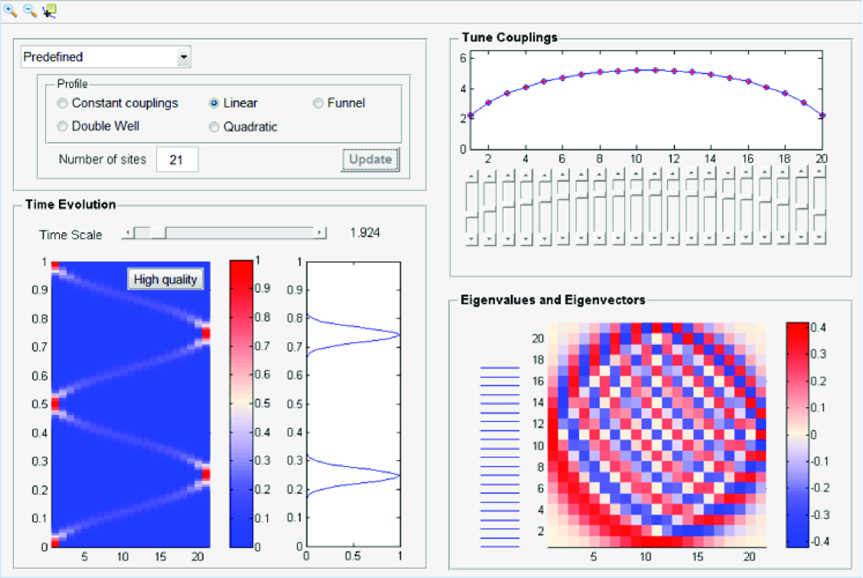
Figure 5: Screenshot of spinGUIn: The upper left panel is used to define the spin chain either via eigenvalues or spin couplings. The remaining panels show (i) the time-evolution of the state including the transfer fidelity (ii) the tunable couplings and (iii) the eigenvalues and eigenstates of the spin chain.