Signature of the long range triplet proximity effect in the density of states

Abstract

We study the impact of the long-range spin-triplet proximity effect on the density of states (DOS) in planar SF₁F₂S Josephson junctions that consist of conventional superconductors (S) connected by two metallic monodomain ferromagnets (F₁ and F₂) with transparent interfaces. We determine the electronic DOS in F layers and the Josephson current for arbitrary orientation of the magnetizations using the solutions of Eilenberger equations in the clean limit and for a moderate disorder in ferromagnets. We find that fully developed long-range proximity effect can occur in highly asymmetric ferromagnetic bilayer Josephson junctions with orthogonal magnetizations. The effect manifests itself as an enhancement in DOS, and as a dominant second harmonic in the Josephson current-phase relation. Distinctive variation of DOS in ferromagnets with the angle between magnetizations is experimentally observable by tunneling spectroscopy. This can provide an unambiguous signature of the long-range spin-triplet proximity effect.

I Introduction

Long-range spin-triplet superconducting correlations induced in heterostructures comprised of superconductors with the usual singlet pairing and inhomogeneous ferromagnets have been predicted recently. Bergeret et al. (2001); Volkov et al. (2003); Bergeret et al. (2005) It has been experimentally verified that superconducting correlations can propagate from SF interfaces with a penetration length up to 1$\mu$m, and provide a nonvanishing Josephson supercurrent through very strong ferromagnets. Sosnin et al. (2006); Keizer et al. (2006); Anwar et al. (2010); Wang et al. (2010); Sprungmann et al. (2010); Khaire et al. (2010); Robinson et al. (2010a)

The simplest Josephson junction with inhomogeneous magnetization is SF₁F₂S structure with monodomain ferromagnetic layers having noncollinear in-plane magnetizations. However, the long-range Josephson effect is not feasible in the junctions with only two F layers,Braude and Nazarov (2007); Houzet and Buzdin (2007); Volkov and Efetov (2010); Pajović et al. (2006); Crouzy et al. (2007) except in highly asymmetric SF₁F₂S junctions at low temperatures, as it was shown in Refs. Trifunovic et al., 2011 and  Trifunovic, 2011. In that case, the long-range spin-triplet effect manifests itself as a large second harmonic ($I_{2}\gg I_{1}$) in the expansion of the Josephson current-phase relation, $I(\phi)=I_{1}\sin(\phi)+I_{2}\sin(2\phi)+\cdots$. The ground state in Josephson junctions with ferromagnetic barriers can be either $0$ or $\pi$ state. The energy of the junction is proportional to $\int_{0}^{\phi}{I(\phi^{\prime})d\phi^{\prime}}$, hence a second harmonic leads to degenerate ground states at $\phi=0$ and $\phi=\pi$. Small contribution of the first harmonic lifts the degeneracy which results in coexistence of stable and metastable $0$ and $\pi$ states.Radović et al. (2001)

In SFS Josephson junctions with homogeneous magnetization, the projection of the total spin of a pair to the direction of magnetization is conserved and only spin-singlet and triplet correlations with zero spin projection occur. Buzdin (2005) These correlations penetrate into the ferromagnet over a short distance (determined by the exchange energy $h$) $\xi_{F}=\hbar v_{F}/h$ in the clean limit and $\xi_{F}=\sqrt{\hbar D/h}$ in the dirty limit, where diffusion coefficient $D=v_{F}l/3$. For inhomogeneous magnetization, odd-frequency triplet correlations with nonzero ($\pm 1$) total spin projection are present as well. These correlations, not suppressed by the exchange interaction, are long-ranged, $\xi_{F}=\hbar v_{F}/k_{B}T$ ($\sqrt{\hbar D/k_{B}T}$) in the clean (dirty) limit, and have a dramatic impact on the Josephson effect. Bergeret et al. (2005)

Dominant influence of long-range triplet correlations on the Josephson current can be realized in SFS junctions with magnetically active interfaces, Eschrig et al. (2003); Eschrig and Löfwander (2008) narrow domain walls between S and thick F interlayers with misaligned magnetizations, Braude and Nazarov (2007); Houzet and Buzdin (2007); Volkov and Efetov (2008, 2010); Trifunovic and Radović (2010); Alidoust and Linder (2010) or superconductors with spin orbit interaction. Duckheim and Brouwer (2011) In addition to the impact on the Josephson current, the odd-frequency triplet pair correlations can be seen through enhanced electronic density of states by tunneling spectroscopy.Cottet (2011) It has been found that proximity effect in diffusive FNS or NFS structures (N is a normal nonmagnetic metal), with magnetically active interface or precessing magnetization, gives a clearcut signature of the odd-frequency superconducting correlations. Yokoyama et al. (2007); Yokoyama and Tserkovnyak (2009) In general, measuring DOS is a very powerful tool to characterize the nature of superconducting correlations in NS and FS structures.Pilgram et al. (2000); Pérez-Willard et al. (2004)

In this article, we study the proximity effect and influence of spin-triplet superconducting correlations in clean and moderately diffusive SF₁F₂S junctions with transparent interfaces. Magnetic interlayer is composed of two monodomain ferromagnets with arbitrary orientation of in-plane magnetizations. We calculate density of states (DOS) in ferromagnetic layers and the Josephson current from the solutions of the Eilenberger equations. Previously, F₁SF₂ and SF₁F₂S junctions with monodomain ferromagnetic layers having noncollinear in-plane magnetizations have been studied using Bogoliubov-de Gennes equation Pajović et al. (2006); Asano et al. (2007); Halterman et al. (2007, 2008) and within the quasiclassical approximation in diffusive Fominov et al. (2003); You et al. (2004); Löfwander et al. (2005); Barash et al. (2002); Fominov et al. (2007); Crouzy et al. (2007); Sperstad et al. (2008); Karminskaya et al. (2009) and clean Blanter and Hekking (2004); Linder et al. (2009) limits using Usadel and Elienberger equations, respectively.

We present analytical solutions in stepwise approximation in the clean limit, and numerical self-consistently obtained results both in the clean limit and for a moderate disorder in ferromagnets. The second harmonic in the Josephson current-phase relation is dominant for highly asymmetric SF₁F₂S junctions composed of particularly thin (weak) and thick (strong) ferromagnetic layers with noncollinear magnetizations. This is a manifestation of the long-range spin-triplet proximity effect at low temperatures, related to the phase coherent transport of two Cooper pairs. Trifunovic et al. (2011); Trifunovic (2011) The proximity effect is also accompanied by pronounced change of both shape and magnitude of electronic DOS in ferromagnetic layers near the Fermi surface. In this case, the self-consistency and finite (but large) electronic mean free path do not alter the analytical results qualitatively. On the other hand, in symmetric SFFS junctions, with equal and strong magnetic influence of F layers, the long-range proximity effect is weak (cannot be dominantTrifunovic et al. (2011)); we show that DOS is therefore equal to its normal metal value even for moderately diffusive ferromagnets.

The article is organized as follows. In Sec. II, we present the model and the equations that we use to calculate the electronic DOS and the Josephson current. In Sec. III, we provide results for different ferromagnetic layers thickness and orientation of magnetizations. The conclusion is given in Sec. IV.

II Model and solutions

We consider a simple model of an SF₁F₂S heterojunction consisting of two conventional ($s$ wave, spin-singlet pairing) superconductors (S) and two uniform monodomain ferromagnetic layers (F₁ and F₂) of thickness $d_{1}$ and $d_{2}$, with angle $\alpha=\alpha_{2}-\alpha_{1}$ between their in-plane magnetizations (see Fig. 1). Interfaces between layers are fully transparent and magnetically inactive.

We describe superconductivity in the framework of the Eilenberger quasiclassical theory. Bergeret et al. (2005); Eilenberger (1966) Ferromagnetism is modeled by the Stoner model, using an exchange energy shift $2h$ between the spin subbands. Disorder is characterized by the electron mean free path $l=v_{F}\tau$, where $\tau$ is the average time between scattering on impurities, and $v_{F}$ is the Fermi velocity assumed to be the same in S and F metals.

Both the clean and moderately diffusive ferromagnetic layers are considered. In the clean limit, the mean free path $l$ is larger than the two characteristic lengths: the ferromagnetic exchange length $\xi_{F}=\hbar v_{F}/h$, and the superconducting coherence length $\xi_{S}=\hbar v_{F}/\pi\Delta_{0}$, where $\Delta_{0}$ is the bulk superconducting pair potential. For moderate disorder, $\xi_{F}<l<\xi_{S}$.

In this model, the Eilenberger Green functions $g_{\sigma\sigma^{\prime}}(x,\theta,\omega_{n})$, $g^{{\dagger}}_{\sigma\sigma^{\prime}}(x,\theta,\omega_{n})$, $f_{\sigma\sigma^{\prime}}(x,\theta,\omega_{n})$, and $f^{{\dagger}}_{\sigma\sigma^{\prime}}(x,\theta,\omega_{n})$ depend on the Cooper pair center-of-mass coordinate $x$ along the junction axis, angle $\theta$ of the quasiclassical trajectories with respect to the $x$ axis, and on the Matsubara frequencies $\omega_{n}=\pi k_{B}T(2n+1)$, $n=0,\pm 1,\ldots$. Spin indices are $\sigma=\uparrow,\downarrow$.

Figure 1: Schematics of an SF₁F₂S heterojunction. The magnetization vectors lie in the y-z plane at angles $\alpha_{1}$ and $\alpha_{2}$ with respect to the $z$-axis.

The Eilenberger equation in particle-hole $\otimes$ spin space can be written in the compact form

$$\hbar v_{x}\partial_{x}\check{g}+\Big{[}\omega_{n}\hat{\tau}_{3}\otimes\hat{1}-i\check{V}-\check{\Delta}+\hbar\langle\check{g}\rangle/2\tau,\check{g}\Big{]}=0,$$ (1)

with normalization condition $\check{g}^{2}=\check{1}$. We indicate by $\hat{\cdots}$ and $\check{\cdots}$ $2\times 2$ and $4\times 4$ matrices, respectively. The brackets $\langle...\rangle=(1/2)\int_{0}^{\pi}(...)\sin(\theta)d\theta$ denote angular averaging over the Fermi surface, $[\;,\;]$ denotes a commutator, and $v_{x}=v_{F}\cos{\theta}$ is the projection of the Fermi velocity vector on the $x$ axis.

The matrix of quasiclassical Green functions isTrifunovic et al. (2011); fUn

$$\check{g}=\left[\begin{array}[]{rrrr}g_{\uparrow\uparrow}&g_{\uparrow\downarrow}&f_{\uparrow\uparrow}&f_{\uparrow\downarrow}\\ g_{\downarrow\uparrow}&g_{\downarrow\downarrow}&f_{\downarrow\uparrow}&f_{\downarrow\downarrow}\\ -f_{\uparrow\uparrow}^{{\dagger}}&-f_{\uparrow\downarrow}^{{\dagger}}&-g_{\uparrow\uparrow}^{{\dagger}}&-g_{\uparrow\downarrow}^{{\dagger}}\\ -f_{\downarrow\uparrow}^{{\dagger}}&-f_{\downarrow\downarrow}^{{\dagger}}&-g_{\downarrow\uparrow}^{{\dagger}}&-g_{\downarrow\downarrow}^{{\dagger}}\end{array}\right],$$ (2)

and the matrix $\check{V}$ is given by

$$\check{V}=\hat{1}\otimes\textrm{Re}\Big{[}\textbf{h}(x)\cdot\widehat{\bm{\sigma}}\Big{]}+i\hat{\tau}_{3}\otimes\textrm{Im}\Big{[}\textbf{h}(x)\cdot\widehat{\bm{\sigma}}\Big{]},$$ (3)

where the components $\hat{\sigma}_{x},\hat{\sigma}_{y},\hat{\sigma}_{z}$ of the vector $\widehat{\bm{\sigma}}$, and $\hat{\tau}_{1},\hat{\tau}_{2},\hat{\tau}_{3}$ are the Pauli matrices in the spin and the particle-hole space, respectively. The in-plane ($y$-$z$) magnetizations of the neighboring F layers are not collinear in general, and form angles $\alpha_{1}$ and $\alpha_{2}$ with respect to the $z$-axis in the left (F₁) and the right (F₂) ferromagnets. The exchange field in ferromagnetic layers is $\textbf{h}(x)=h_{1}(0,\sin{\alpha_{1}},\cos{\alpha_{1}})$ and $h_{2}(0,\sin{\alpha_{2}},\cos{\alpha_{2}})$.

We assume that the superconductors are identical, with

$$\check{\Delta}=\left[\begin{array}[]{cc}0&\hat{\sigma}_{2}\Delta\\ \hat{\sigma}_{2}\Delta^{*}&0\end{array}\right]$$ (4)

for $x<-d_{1}$ and $x>d_{2}$. The self-consistency condition for the pair potential $\Delta=\Delta(x)$ is given by

$$\Delta=-i\lambda\pi N_{0}(0)k_{B}T\sum_{\omega_{n}}\langle f_{\uparrow\downarrow}\rangle,$$ (5)

where $\lambda$ is the coupling constant, $N_{0}(0)=mk_{F}/\pi^{2}\hbar^{2}$ is the density of states (per unit volume) of the free electron gas at the Fermi level $E_{F}=\hbar^{2}k_{F}^{2}/2m$, and $k_{F}=mv_{F}/\hbar$ is the Fermi wave number. In F layers $\check{\Delta}=0$.

The density of states normalized by its normal-state value is given by analytical continuation

$$N(\varepsilon)/N_{0}(0)=\frac{1}{2}\;\sum_{\sigma}\langle\textrm{Re}\hskip 2.84526ptg_{\sigma\sigma}(i\omega_{n}\to\varepsilon+i\delta)\rangle,$$ (6)

where a small imaginary part of the energy is introduced to regularize singularities. In numerical calculations we choose $\delta/\Delta_{0}(0)=10^{-2}$.

The supercurrent is obtained from the normal Green function through the following expression

$$I(\phi)=\frac{1}{2}\pi eN_{0}(0)Sk_{B}T\sum_{\omega_{n}}\sum_{\sigma}\langle v_{x}\textrm{Im}\hskip 2.84526ptg_{\sigma\sigma}\rangle,$$ (7)

where $\phi$ is the macroscopic phase difference across the junction, and $S$ is the area of the junction. In our examples, the current is normalized to $\pi\Delta_{0}/eR_{N}$ where $R_{N}=2\pi^{2}\hbar/Se^{2}k_{F}^{2}$.

We consider only transparent interfaces and use continuity of the Green functions as the boundary conditions. Analytical solutions of Eq. (1) are derived (see Appendix) in the stepwise approximation for the pair potential

$$\Delta=\Delta_{0}\left[e^{-i\phi/2}\Theta(-x-d_{1})+e^{i\phi/2}\Theta(x-d_{2})\right],$$ (8)

where $\Delta_{0}$ is the bulk pair potential, and $\Theta(x)$ is the Heaviside step function. The temperature dependence of the bulk pair potential $\Delta_{0}$ is given by $\Delta_{0}(T)=\Delta_{0}(0)\tanh\left(1.74\sqrt{T_{c}/T-1}\right)$. Mühlschlegel (1959)

We have chosen $\alpha_{2}=0$, that is $\alpha=\alpha_{1}$. For three characteristic values of the angle between magnetizations $\alpha=0$, $\pi/2$, and $\pi$, the normal Green functions in F₂ layer are $x$-independent and can be written in a compact form

$$g_{\sigma\sigma}(\theta,\omega_{n})=\frac{\omega_{n}}{\Omega_{n}}+\frac{\Delta_{0}^{2}}{\Omega_{n}}\;\frac{1}{\omega_{n}+i\Omega_{n}\hskip 2.84526pt\hbox{sign}(\cos{\theta})\cot{\left(\pm\frac{\vartheta_{1}+\vartheta_{2}}{2}+i\frac{\Xi_{n}}{2}-\frac{\phi}{2}\right)}},$$ (9)

$$g_{\sigma\sigma}(\theta,\omega_{n})=\frac{\omega_{n}}{\Omega_{n}}+\frac{\Delta_{0}^{2}}{\Omega_{n}}\;\frac{\omega_{n}[\cos{(\phi-i\Xi_{n})}-\cos{(\vartheta_{1})}\cos{(\vartheta_{2})}]-i\Omega_{n}\hskip 2.84526pt\hbox{sign}(\cos{\theta})[\pm\cos{(\vartheta_{1})}\sin{(\vartheta_{2})}-\sin{(\phi-i\Xi_{n})}]}{(\Omega_{n}^{2}+\omega_{n}^{2})\cos{(\phi-i\Xi_{n})}+(\Omega_{n}^{2}-\omega_{n}^{2})\cos{(\vartheta_{1})}\cos{(\vartheta_{2})}+2i\omega_{n}\Omega_{n}\hskip 2.84526pt\hbox{sign}(\cos{\theta})\sin{(\phi-i\Xi_{n})}},$$ (10)

$$g_{\sigma\sigma}(\theta,\omega_{n})=\frac{\omega_{n}}{\Omega_{n}}+\frac{\Delta_{0}^{2}}{\Omega_{n}}\;\frac{1}{\omega_{n}+i\Omega_{n}\hskip 2.84526pt\hbox{sign}(\cos{\theta})\cot{\left(\pm\frac{\vartheta_{2}-\vartheta_{1}}{2}+i\frac{\Xi_{n}}{2}-\frac{\phi}{2}\right)}},$$ (11)

respectively. Here, $\pm$ corresponds to $\sigma=\uparrow,\downarrow$, $\Omega_{n}^{2}=\omega_{n}^{2}+\Delta_{0}^{2}$, $\Xi_{n}=2(d_{1}+d_{2})\omega_{n}/\hbar v_{F}\cos{\theta}$ and $\vartheta_{j}=2d_{j}h_{j}/\hbar v_{F}\cos{\theta}$, $j=1$, $2$.

The well-known normal Green functions for $\alpha=0$ and $\pi$ are the same in F₁ and F₂ layers, Eqs. (9) and (11).Konschelle et al. (2008); Blanter and Hekking (2004) However, for $\alpha=\pi/2$ only $\sum_{\sigma}g_{\sigma\sigma}$ is the same in F₁ and F₂. In F₁ layer, $g_{\sigma\sigma}$ is $x$- and $\sigma$-dependent and cannot be expressed in a compact form.

The energy of Andreev states is determined by the poles of the Green functions. In contrast to the case of collinear magnetizations, the spin splitting of Andreev states is absent for orthogonal magnetizations, Eq. (10), where the long-range spin-triplet proximity effect is maximally pronounced.

Real part of the Green functions as a function of energy $\varepsilon$ inside the superconducting gap, $-\Delta_{0}<\varepsilon<\Delta_{0}$, reduces to four delta functions with $\theta$-dependent position for collinear magnetizations, and two delta functions for orthogonal magentizations. For planar SF₁F₂S junctions these contributions should be numerically summed over $\theta$. Note that the electronic DOS in ferromagnets is independent of $x$ only in the clean limit. For a finite electronic mean free path, DOS is calculated in the middle of F₂ ferromagnetic layer.

The above results for DOS in the clean limit, obtained in the stepwise approximation for the pair potential, are not altered qualitatively in numerical self-consistent calculations. Numerical computation for both the clean limit and for moderately diffusive ferromagnets is carried out using the collocation method: Eq. (1) is solved iteratively together with the self-consistency condition, Eq. (5). Iterations are performed until self-consistency is reached, starting from the stepwise approximation for the pair potential. For a finite electron mean free path in ferromagnets, the iterative procedure starts from the clean limit. We choose the appropriate boundary conditions in superconductors at the distance exceeding $2\xi_{S}$ from the SF interfaces. These boundary conditions are determined by eliminating the unknown constants from the analytical solutions in stepwise approximation. To reach self-consistency with good accuracy, starting from the stepwise $\Delta$, five to ten iterative steps were sufficient.

III Results

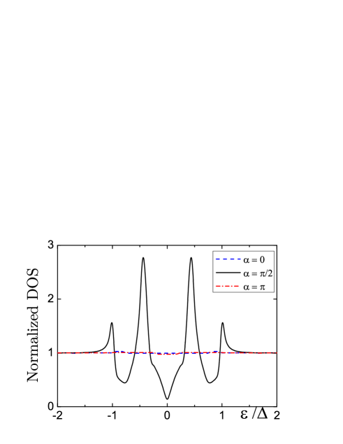
Figure 2: (Color online) Normalized DOS, $N(\varepsilon)/N_{0}(0)$, in ferromagnets for an asymmetric SF₁F₂S junction with $d_{1}=10k_{F}^{-1}$ and $d_{2}=990k_{F}^{-1}$, $h_{1}=h_{2}=0.1E_{F}$. Superconductor is characterized by $\Delta_{0}(0)/E_{\rm F}=10^{-3}$; the phase difference $\phi=0$. The results of non-self-consistent calculations in the clean limit, $l\to\infty$, are shown for three values of the relative angle between magnetizations: $\alpha=0$ (dashed curve), $\pi/2$ (solid curve), and $\pi$ (dash-dotted curve).

We illustrate our results on SF₁F₂S planar junctions with relatively weak ferromagnets, $h/E_{F}=0.1$, and the ferromagnetic exchange length $\xi_{F}=20k_{F}^{-1}$. Superconductors are characterized by the bulk pair potential at zero temperature $\Delta_{0}(0)/E_{\rm F}=10^{-3}$, which corresponds to the superconducting coherence length $\xi_{S}(0)=636k_{F}^{-1}$. We assume that all interfaces are fully transparent and the Fermi wave numbers in all metals are equal ($k_{F}^{-1}\sim$ 1Å).

Detailed analysis is given for a highly asymmetric junction ($d_{1}=10k_{F}^{-1}$ and $d_{2}=990k_{F}^{-1}$), Figs. 2-4, and for a symmetric junction ($d_{1}=d_{2}=500k_{F}^{-1}$), Figs. 5 and 6. In these examples: $h_{1}=h_{2}=0.1E_{F}$ and $T/T_{c}=0.1$. In Figs. 2, 3, and 5, the results of non-self-consistent calculations for DOS and Josephson currents are shown in the clean limit ($l\rightarrow\infty$). The self-consistent numerical calculations for electronic DOS in the clean limit ($l\rightarrow\infty$) and for moderate disorder ($l=200k_{F}^{-1}$) in ferromagnets are shown in Figs. 4 and 6.

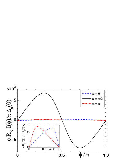
Figure 3: (Color online) The Josephson current-phase relation $I(\phi)$ for an asymmetric SF₁F₂S junction with $d_{1}=10k_{F}^{-1}$ and $d_{2}=990k_{F}^{-1}$, $h_{1}=h_{2}=0.1E_{F}$, $l\to\infty$, $T/T_{c}=0.1$, and for three values of the relative angle between magnetizations: $\alpha=0$ (dashed curve), $\pi/2$ (solid curve), and $\pi$ (dash-dotted curve). Inset: Magnified curves for $\alpha=0$ and $\alpha=\pi$.

Figure 4: Normalized DOS, $N(\varepsilon)/N_{0}(0)$, in ferromagnets for an asymmetric SF₁F₂S junction with $d_{1}=10k_{F}^{-1}$ and $d_{2}=990k_{F}^{-1}$, $h_{1}=h_{2}=0.1E_{F}$, for $\alpha=\pi/2$. Superconductor is characterized by $\Delta_{0}(0)/E_{\rm F}=10^{-3}$; the phase difference $\phi=0$. Results of self-consistent numerical solutions in the clean limit, $l\to\infty$ (thin solid curve) and for moderately diffusive ferromagnets, $l=200k_{F}^{-1}$, $x=d_{2}/2$ (thick solid curve) are shown. For comparison, the non-self-consistent solution in the clean limit (dotted curve) is also shown.

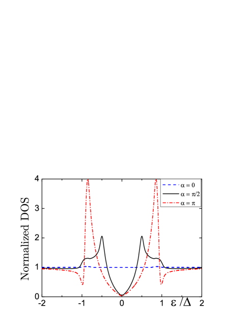
Figure 5: (Color online) Normalized DOS, $N(\varepsilon)/N_{0}(0)$, in ferromagnets for a symmetric SF₁F₂S junction with $d_{1}=d_{2}=500k_{F}^{-1}$, $h_{1}=h_{2}=0.1E_{F}$. Superconductor is characterized by $\Delta_{0}(0)/E_{\rm F}=10^{-3}$; the phase difference $\phi=0$. Results of non-self-consistent calculations in the clean limit, $l\to\infty$ are shown for three values of the relative angle between magnetizations: $\alpha=0$ (dashed curve), $\pi/2$ (solid curve), and $\pi$ (dash-dotted curve).

Figure 6: Normalized DOS, $N(\varepsilon)/N_{0}(0)$, in ferromagnets for a symmetric SF₁F₂S junction with $d_{1}=d_{2}=500k_{F}^{-1}$, $h_{1}=h_{2}=0.1E_{F}$, for $\alpha=\pi/2$. Superconductor is characterized by $\Delta_{0}(0)/E_{\rm F}=10^{-3}$; the phase difference $\phi=0$. Results of self-consistent numerical solutions in the clean limit, $l\to\infty$ (thin solid curve) and for moderately diffusive ferromagnets, $l=200k_{F}^{-1}$, $x=d_{2}/2$ (thick solid curve) are shown. For comparison, the non-self-consistent solution in the clean limit (dotted curve) is also shown.

In highly asymmetric SF₁F₂S junctions the variation of DOS for finite electronic mean free path is less pronounced but qualitatively similar to the clean limit results, see Fig. 4. This is not the case for symmetric junctions where the long-range spin-triplet proximity effect is weak, Fig. 6.

Influence of the ferromagnet is predominantly determined by the parameter $\Theta=(h/E_{F})k_{F}d$, and the results shown here remain the same for a large range of the junction parameters where $\Theta_{1}\sim 1$ in F₁ and $\Theta_{2}\sim 100$ in F₂ layers. Note that $\Theta_{1}\sim 1$ is the optimal choice for long-range triplet Josephson effect. Trifunovic and Radović (2010) For experimental realization of asymmetric junctions it is more suitable to use weak and strong ferromagnets ($h_{1}\ll h_{2}$) with small and comparable thickness ($d_{1}\approx d_{2}$) to avoid multidomain magnetic structures and destructive influence of the orbital effect (vortices). Lyuksyutov and Pokrovsky (2005)

We have verified by additional calculations that the long-range triplet proximity effect in highly asymmetric SF₁F₂S junctions is rather robust. Small variations in the layers thickness and in the exchange energy of ferromagnets, as well as moderate disorder, do not affect distinctive feature of DOS. Likewise, the long-ranged second harmonic in $I(\phi)$ at low temperatures remains dominant.Trifunovic et al. (2011)

In all calculations we have assumed transparent SF interfaces and clean or moderately disordered ferromagnets. Finite transparency, as well as large disorder, strongly suppress the Josephson current and the electronic DOS approaches its normal state value.

In symmetric SFFS junctions with equal ferromagnetic layers no substantial impact of long-range spin-triplet superconducting correlations on the Josephson current has been found previously both in the ballistic and diffusive regimes. Pajović et al. (2006); Crouzy et al. (2007); Trifunovic et al. (2011); Trifunovic (2011) It can be seen from Figs. 5 and 6 that the electronic DOS for $\alpha=\pi/2$ is much less pronounced than for the corresponding (equal strength and total thickness of ferromagnets) asymmetric junction, Figs. 2 and 3. Moreover, for moderate disorder in ferromagnts, $l=200k_{F}^{-1}$, the proximity effect is practically absent, and DOS equals its normal value (Fig. 6). In symmetric SFFS junctions the Josephson critical current monotonically increases with angle between the magnetizations, except in the vicinity of $0-\pi$ transitions. Trifunovic et al. (2011) In the clean limit for $\alpha=\pi$, the influence of opposite magnetizations in F layers practically cancels out and the proximity effect is much stronger, see Fig. 5. Both DOS and the Josephson current-phase relation are the same as for the corresponding SNS junction, where N stands for a normal nonmagnetic metal ($h_{1}=h_{2}=0$). Recently, substantially enhanced supercurrent has been observed in Josephson junctions with ferromagnetic Fe/Cr/Fe trilayer in the antiparallel configuration, without long-range spin-triplet correlations. Robinson et al. (2010b)

IV Conclusion

We have studied the spin-triplet proximity effect in SF₁F₂S planar junctions made of conventional superconductors and two monodomain ferromagnetic layers with arbitrary thickness, strength, and angle between in-plane magnetizations. We have derived analytical expressions for the quasiclassical normal Green functions in the clean limit and the stepwise pair potential approximation (non self-consistent). We have calculated the electronic density of states in ferromagnets, and the Josephson current. In addition, results of the numerical self-consistent calculations for the clean and moderately diffusive ferromagnets are shown for comparison.

The second harmonic in the Josephson current-phase relation is dominant for highly asymmetric SF₁F₂S junctions composed of particularly thin (weak) and thick (strong) ferromagnetic layers with noncollinear magnetizations. This is a manifestation of the long-range spin-triplet proximity effect at low temperatures, related to the phase coherent transport of two Cooper pairs. We find that the proximity effect is also accompanied by distinctive variation of electronic DOS in ferromagnetic layers as a function of energy near the Fermi surface. This variation is less pronounced in moderately diffusive case, but still detectable by tunneling spectroscopy as a signature of the long-range proximity effect. The self-consistency and finite (but large) electronic mean free path do not alter the analytical results qualitatively. In contrast, in symmetric junctions with moderately diffusive and thick ferromagnets the long-range proximity effect is absent and DOS is equal to its normal metal value.

In summary, fully developed long-range proximity effect occurs in highly asymmetric SF₁F₂S junctions with orthogonal magentizations. Dominant second harmonic in the Josephson current-phase relation, as well as a distinctive variation of DOS in ferromagnetic layers with the angle between magnetizations, should be experimentally observable for relatively small interface roughness and relatively clean ferromagnetic layers at low temperatures.

V Acknowledgment

The work was supported by the Serbian Ministry of Science, Project No. 171027. Z. R. acknowledges Mihajlo Vanević, Ivan Božović, and Marco Aprili for helpful discussions.

VI Appendix

In the clean limit, $l\rightarrow\infty$, solutions of Eq. (1) in the step-wise approximation, Eq. (8), for the left superconductor ($x<-d_{1}$) can be written in the usual form for normal Green functions

$$g_{\uparrow\uparrow}(x) = \frac{\omega_{n}}{\Omega_{n}}+D_{1}e^{\kappa_{s}x},$$ (12)

$$g_{\uparrow\downarrow}(x) = D_{2}e^{\kappa_{s}x},$$ (13)

$$g_{\downarrow\uparrow}(x) = D_{3}e^{\kappa_{s}x},$$ (14)

$$g_{\downarrow\downarrow}(x) = \frac{\omega_{n}}{\Omega_{n}}+D_{4}e^{\kappa_{s}x},$$ (15)

and for anomalous Green functions

$$f_{\uparrow\uparrow}(x) = -\frac{2i\Delta_{0}}{2\omega_{n}+\hbar v_{x}\kappa_{s}}D_{2}e^{\kappa_{s}x},$$ (16)

$$f_{\uparrow\downarrow}(x) = \frac{i\Delta_{0}}{\Omega_{n}}+\frac{2i\Delta_{0}}{2\omega_{n}+\hbar v_{x}\kappa_{s}}D_{1}e^{\kappa_{s}x},$$ (17)

$$f_{\downarrow\uparrow}(x) = -\frac{i\Delta_{0}}{\Omega_{n}}-\frac{2i\Delta_{0}}{2\omega_{n}+\hbar v_{x}\kappa_{s}}D_{4}e^{\kappa_{s}x},$$ (18)

$$f_{\downarrow\downarrow}(x) = \frac{2i\Delta_{0}}{2\omega_{n}+\hbar v_{x}\kappa_{s}}D_{3}e^{\kappa_{s}x},$$ (19)

with

$$\kappa_{s}=\frac{2\Omega_{n}}{\hbar v_{F}|\cos(\theta)|},$$ (20)

and $\Omega_{n}=\sqrt{\omega_{n}^{2}+|\Delta|^{2}}$. For the right superconductor ($x>d_{2}$), the solutions retain the same form with $\kappa_{s}\longrightarrow-\kappa_{s}$, $\phi\longrightarrow-\phi$, with a new set of constants $D^{\prime}_{1},...,D^{\prime}_{4}$.

Solutions for the Green functions in the left ferromagnetic layer F₁, $-d_{1}<x<0$, for three values of angle $\alpha_{1}=0$, $\pi/2$, $\pi$ (we have chosen $\alpha_{2}=0$) can be written as follows. For collinear magnetizations $\alpha_{1}=0$ and $\pi$,

$$g_{\uparrow\uparrow}(x) = K_{1},$$ (21)

$$g_{\uparrow\downarrow}(x) = K_{2}e^{\pm i\kappa_{0}x},$$ (22)

$$g_{\downarrow\uparrow}(x) = K_{3}e^{\mp i\kappa_{0}x},$$ (23)

$$g_{\downarrow\downarrow}(x) = K_{4},$$ (24)

and

$$f_{\uparrow\uparrow}(x) = C_{1}e^{i\kappa x},$$ (25)

$$f_{\uparrow\downarrow}(x) = C_{2}e^{i\kappa_{\pm}x},$$ (26)

$$f_{\downarrow\uparrow}(x) = C_{3}e^{i\kappa_{\mp}x},$$ (27)

$$f_{\downarrow\downarrow}(x) = C_{4}e^{i\kappa x},$$ (28)

where the upper (lower) sign corresponds to $\alpha_{1}=0$ ($\alpha_{1}=\pi$). For orthogonal magnetizations, $\alpha_{1}=\pi/2$,

$$g_{\uparrow\uparrow}(x) = K_{1}+K_{2}e^{i\kappa_{0}x}+K_{3}e^{-i\kappa_{0}x},$$ (29)

$$g_{\uparrow\downarrow}(x) = K_{4}+iK_{2}e^{i\kappa_{0}x}-iK_{3}e^{-i\kappa_{0}x},$$ (30)

$$g_{\downarrow\uparrow}(x) = -K_{4}+iK_{2}e^{i\kappa_{0}x}-iK_{3}e^{-i\kappa_{0}x},$$ (31)

$$g_{\downarrow\downarrow}(x) = K_{1}-K_{2}e^{i\kappa_{0}x}-K_{3}e^{-i\kappa_{0}x},$$ (32)

and

$$f_{\uparrow\uparrow}(x) = C_{1}e^{i\kappa x}+C_{2}e^{i\kappa_{+}x}+C_{3}e^{i\kappa_{-}x},$$ (33)

$$f_{\uparrow\downarrow}(x) = C_{4}e^{i\kappa x}-iC_{2}e^{i\kappa_{+}x}+iC_{3}e^{i\kappa_{-}x},$$ (34)

$$f_{\downarrow\uparrow}(x) = C_{4}e^{i\kappa x}+iC_{2}e^{i\kappa_{+}x}-iC_{3}e^{i\kappa_{-}x},$$ (35)

$$f_{\downarrow\downarrow}(x) = -C_{1}e^{i\kappa x}+C_{2}e^{i\kappa_{+}x}+C_{3}e^{i\kappa_{-}x}.$$ (36)

Here,

$$\kappa_{0} = 2h_{1}/\hbar v_{x},$$ (37)

$$\kappa = 2i\omega_{n}/\hbar v_{x},$$ (38)

$$\kappa_{\pm} = 2(i\omega_{n}\pm h_{1})/\hbar v_{x}.$$ (39)

For the right ferromagnetic layer F₂, $0<x<d_{2}$, $\alpha_{2}=0$, the solutions are the same as for the layer F₁ in the case $\alpha_{1}=0$, with $h_{1}\to h_{2}$ and a new set of constants $K^{\prime}_{1},\ldots,K^{\prime}_{4}$, $C^{\prime}_{1},\ldots,C^{\prime}_{4}$.

The complete solution has $24$ unknown coefficients: $4+4$ in superconducting electrodes, and $8+8$ in ferromagnetic layers. Continuity of normal and anomalous Green functions at the three interfaces provide the necessary set of $24$ equations.

References

- Bergeret et al. (2001) F. S. Bergeret, A. F. Volkov, and K. B. Efetov, Phys. Rev. Lett. 86, 4096 (2001).
- Volkov et al. (2003) A. F. Volkov, F. S. Bergeret, and K. B. Efetov, Phys. Rev. Lett. 90, 117006 (2003).
- Bergeret et al. (2005) F. S. Bergeret, A. F. Volkov, and K. B. Efetov, Rev. Mod. Phys. 77, 1321 (2005).
- Sosnin et al. (2006) I. Sosnin, H. Cho, V. T. Petrashov, and A. F. Volkov, Phys. Rev. Lett. 96, 157002 (2006).
- Keizer et al. (2006) R. S. Keizer, S. T. B. Goennenwein, T. M. Klapwijk, G. Miao, G. Xiao, and A. Gupta, Nature 439, 825 (2006).
- Anwar et al. (2010) M. S. Anwar, F. Czeschka, M. Hesselberth, M. Porcu, and J. Aarts, Phys. Rev. B 82, 100501 (2010).
- Wang et al. (2010) J. Wang, M. Singh, M. Tian, N. Kumar, B. Liu, C. Shi, J. K. Jain, N. Samarth, T. E. Mallouk, and M. H. W. Chan, Nature Phys. 6, 389 (2010).
- Sprungmann et al. (2010) D. Sprungmann, K. Westerholt, H. Zabel, M. Weides, and H. Kohlstedt, Phys. Rev. B 82, 060505(R) (2010).
- Khaire et al. (2010) T. S. Khaire, M. A. Khasawneh, W. P. Pratt, and N. O. Birge, Phys. Rev. Lett. 104, 137002 (2010).
- Robinson et al. (2010a) J. W. A. Robinson, J. D. S. Witt, and M. G. Blamire, Science 329, 59 (2010a).
- Braude and Nazarov (2007) V. Braude and Y. V. Nazarov, Phys. Rev. Lett. 98, 077003 (2007).
- Houzet and Buzdin (2007) M. Houzet and A. I. Buzdin, Phys. Rev. B 76, 060504 (2007).
- Volkov and Efetov (2010) A. F. Volkov and K. B. Efetov, Phys. Rev. B 81, 144522 (2010).
- Pajović et al. (2006) Z. Pajović, M. Božović, Z. Radović, J. Cayssol, and A. Buzdin, Phys. Rev. B 74, 184509 (2006).
- Crouzy et al. (2007) B. Crouzy, S. Tollis, and D. A. Ivanov, Phys. Rev. B 75, 054503 (2007).
- Trifunovic et al. (2011) L. Trifunovic, Z. Popović, and Z. Radović, Phys. Rev. B 84, 064511 (2011).
- Trifunovic (2011) L. Trifunovic, Phys. Rev. Lett. 107, 047001 (2011).
- Radović et al. (2001) Z. Radović, L. Dobrosavljević-Grujić, and B. Vujičić, Phys. Rev. B 63, 214512 (2001).
- Buzdin (2005) A. I. Buzdin, Rev. Mod. Phys. 77, 935 (2005).
- Eschrig et al. (2003) M. Eschrig, J. Kopu, J. C. Cuevas, and G. Schön, Phys. Rev. Lett. 90, 137003 (2003).
- Eschrig and Löfwander (2008) M. Eschrig and T. Löfwander, Nature Phys. 4, 138 (2008).
- Volkov and Efetov (2008) A. F. Volkov and K. B. Efetov, Phys. Rev. B 78, 024519 (2008).
- Trifunovic and Radović (2010) L. Trifunovic and Z. Radović, Phys. Rev. B 82, 020505 (2010).
- Alidoust and Linder (2010) M. Alidoust and J. Linder, Phys. Rev. B 82, 224504 (2010).
- Duckheim and Brouwer (2011) M. Duckheim and P. W. Brouwer, Phys. Rev. B 83, 054513 (2011).
- Cottet (2011) A. Cottet, Phys. Rev. Lett. 107, 177001 (2011).
- Yokoyama et al. (2007) T. Yokoyama, Y. Tanaka, and A. A. Golubov, Phys. Rev. B 75, 134510 (2007).
- Yokoyama and Tserkovnyak (2009) T. Yokoyama and Y. Tserkovnyak, Phys. Rev. B 80, 104416 (2009).
- Pilgram et al. (2000) S. Pilgram, W. Belzig, and C. Bruder, Phys. Rev. B 62, 12462 (2000).
- Pérez-Willard et al. (2004) F. Pérez-Willard, J. C. Cuevas, C. Sürgers, P. Pfundstein, J. Kopu, M. Eschrig, and H. v. Löhneysen, Phys. Rev. B 69, 140502 (2004).
- Asano et al. (2007) Y. Asano, Y. Tanaka, and A. A. Golubov, Phys. Rev. Lett. 98, 107002 (2007).
- Halterman et al. (2007) K. Halterman, P. H. Barsic, and O. T. Valls, Phys. Rev. Lett. 99, 127002 (2007).
- Halterman et al. (2008) K. Halterman, O. T. Valls, and P. H. Barsic, Phys. Rev. B 77, 174511 (2008).
- Fominov et al. (2003) Y. Fominov, A. Golubov, and M. Kupriyanov, JETP Lett. 77, 510 (2003).
- You et al. (2004) C. You, Y. B. Bazaliy, J. Y. Gu, S. Oh, L. M. Litvak, and S. D. Bader, Phys. Rev. B 70, 014505 (2004).
- Löfwander et al. (2005) T. Löfwander, T. Champel, J. Durst, and M. Eschrig, Phys. Rev. Lett. 95, 187003 (2005).
- Barash et al. (2002) Y. S. Barash, I. V. Bobkova, and T. Kopp, Phys. Rev. B 66, 140503 (2002).
- Fominov et al. (2007) Y. V. Fominov, A. F. Volkov, and K. B. Efetov, Phys. Rev. B 75, 104509 (2007).
- Sperstad et al. (2008) I. B. Sperstad, J. Linder, and A. Sudbø, Phys. Rev. B 78, 104509 (2008).
- Karminskaya et al. (2009) T. Y. Karminskaya, A. A. Golubov, M. Y. Kupriyanov, and A. S. Sidorenko, Phys. Rev. B 79, 214509 (2009).
- Blanter and Hekking (2004) Y. M. Blanter and F. W. J. Hekking, Phys. Rev. B 69, 024525 (2004).
- Linder et al. (2009) J. Linder, M. Zareyan, and A. Sudbø, Phys. Rev. B 79, 064514 (2009).
- Eilenberger (1966) G. Eilenberger, Z. Phys. 190, 142 (1966).
- (44) Our matrix and Eq. (1) are equivalent up to an unitary transformation to the definitions used in Ref. Bergeret et al., 2005.
- Mühlschlegel (1959) B. Mühlschlegel, Z. Phys. 155, 313 (1959).
- Konschelle et al. (2008) F. Konschelle, J. Cayssol, and A. I. Buzdin, Phys. Rev. B 78, 134505 (2008).
- Lyuksyutov and Pokrovsky (2005) I. F. Lyuksyutov and V. L. Pokrovsky, Adv. Phys. 54, 67 (2005).
- Robinson et al. (2010b) J. W. A. Robinson, G. B. Halász, A. I. Buzdin, and M. G. Blamire, Phys. Rev. Lett. 104, 207001 (2010b).