Oracle inequalities and minimax rates for non-local means
and related adaptive kernel-based methods

Abstract

This paper describes a novel theoretical characterization of the performance of non-local means (NLM) for noise removal. NLM has proven effective in a variety of empirical studies, but little is understood fundamentally about how it performs relative to classical methods based on wavelets or how its parameters should be chosen. For cartoon images and images which may contain thin features and regular textures, the error decay rates of NLM are derived and compared with those of linear filtering, oracle estimators, Yaroslavsky’s filter and wavelet thresholding estimators. The trade-off between global and local search for matching patches is examined, and the bias reduction associated with the local polynomial regression version of NLM is analyzed. The theoretical results are validated via simulations for 2D images corrupted by additive white Gaussian noise.

1 Introduction

The classical problem of image noise removal has drawn significant attention during the past few decades from the image processing, computational harmonic analysis, nonlinear approximation, and statistics communities. In recent years there has been a resurgence of interest in kernel-based methods, including the ubiquitous non-local means (NLM) algorithm [6], due to their practical efficacy on broad collections of “natural” images. While there is a wealth of theoretical analysis associated with nonlinear thresholding estimators based on wavelets and related sparse multiscale representations of images [13, 14, 35, 51] or on diffusion models [52, 47] and partial differential equations [39, 1], performance guarantees for NLM are lacking and this paper aims at providing some results in this direction.

In this paper, we explore the theoretical underpinnings of adaptive kernel-based image estimation and derive bounds on the mean squared error as a function of the number of pixels observed and features of the underlying image. The denoising methods we consider are based on estimating each pixel value with a weighted sum of the surrounding pixels. Depending on how the weights in this average are selected, this corresponds to classical linear filters [38, 60], Yaroslavsky’s filter (YF) [62], the Sigma filter [28], or the bilateral filter [55]. It also includes variable-bandwidth kernel estimators [29], referred to as Lepski’s method by statisticians and as the Intersection of Confidence Intervals (ICI) rule [22, 23] in signal processing. Other variants for a local choice of the kernel include [49, 53] We refer to [20, 43, 36] for more insights on a unifying framework for averaging filters.

As none of these methods have been explicitly designed to deal with textured regions, many authors, inspired by work on texture synthesis [16] and inpainting [8], have proposed to introduce patches (small sub-images) to take advantage of natural image redundancy, especially in textured regions. NLM [6] and UINTA [3] algorithms are typical examples of this approach, as is their extension using Lepski’s method [26]. Those algorithms rely on averaging similar pixels, where the similarity is measured through patches centered on the pixel of interest. Some more elaborate methods have tried to remove artifacts appearing in regions with low redundancy [45] — a phenomenon also known as the rare patch effect [15] — for instance by choosing NLM parameters automatically and locally. A common tool used for this local adaptivity is the Stein Unbiased Risk Estimate (SURE) [15, 58, 59].

Most current state-of-the-art methods for denoising take advantage of the patch framework [32, 9, 10]. The interested reader could get a clear picture of practical performance of those recent methods, in the review paper by Katkovnik et al. [25]. Despite the strong empirical performance of these methods, few performance guarantees exist: bounds with information theory flavor are derived in [61] for a simple version of NLM; a consistency result relying on beta-mixing assumptions on the image and on the noise (both modeled as random variables) is obtained in [5, 6]; [47] proposes a graph-diffusion interpretation for a simple image model; a bias/variance analysis aiming at locally choosing NLM parameters is carried out in [15]; [30, 7] obtain Cramer-Rao type efficiency results. While finishing this paper, we became aware of two related papers by Maleki, Narayan and Baraniuk, addressing optimal performance in the context of non-parametric minimax estimation [34, 33]. [34] evaluates the performance of NLM for the piecewise constant horizon model [27], while [33] considers an anisotropic variant of NLM for the same image class. The latter shares several features with earlier work on anisotropic NLM [11, 12]. Our work is most closely related to [34], addressing the same challenge of quantifying the performance of NLM and related methods, and at the same time contains several novel contributions. While the paper was under review, we learned about an older paper of Tsybakov [56]. This paper proposes and analyzes a patch-based method that compares the medians over patches. The paper also derives a minimax lower bound for the cartoon model we consider. We comment in more detail on the work of Maleki [34] et al and the work of Tsybakov [56] in Section 7.

1.1 Our contribution

We derive theoretical performance bounds for the linear filter, oracle variable-bandwidth kernel methods, Yaroslavsky’s filter and NLM — both the original [6] and a fast patch-mean based variant [31] — in the classical “cartoon” model in which an image consists of smooth surfaces separated by a smooth discontinuity, a popular model in statistics [27]. Our results are for the local polynomial versions of these methods. (The systematic bias associated with NLM near discontinuities — and boundaries — is shown to disappear when using a local polynomial regression.) We also consider nonstandard image classes, one modeling images with thin features and another one modeling regular textures. The latter is particularly significant because it highlights some of the key advantages of patch-based methods over, say, wavelet thresholding estimators. Previous insights into the performance of NLM-like methods on textures are empirical at best; we are not aware of any theory in this vein. Our benchmarks are two oracle inequalities, though many of our theoretical results can be compared directly with similar classical results in the wavelet literature and known minimax lower bounds on mean squared error (MSE) [14, 27].

The cartoon model for images has been a benchmark for image denoising methods, at least since the work of Korostelev and Tsybakov, condensed in [27]. This model is relevant when comparing denoising methods on texture-less images. The other models are novel and tailored to situations where the image exhibits some thin features — like the legs of the Cameraman’s tripod — and regular textures — like the patterns in Barbara’s blouse. Though these models do not reflect the complexities of real images, we do gain some qualitative insights. First, we learn that variable bandwidth kernel methods are fundamentally limited by the bias near discontinuities. Yaroslavsky’s filter is found to be near-optimal when the noise level is sufficiently low that the different regions in the cartoon image do not mix when noise is added; and when this is not the case, the method becomes useless. In non-local means, the patch size should be chosen just sufficiently large that nearby patches from different regions look different (in the average version of the NLM, this can be made very precise). The search window should be chosen like a standard kernel bandwidth. We quickly argue that not localizing these methods may lead to very poor performance, in agreement with [44, 64]. Also, while the NLM average and regular NLM perform similarly on cartoon images, the latter is superior when textures are present.

1.2 Organization of the paper

In Section 2 we describe the mathematical framework. In Section 3 we introduce the methods that we analyze in the sequel. In Section 4 we state performance guarantees in the cartoon model for these methods, and in Section 5 we do the same in the context of the thin feature and regular pattern models. In Section 6 we perform some numerical experiments carefully illustrating our theoretical findings. In Section 7 we contrast our contribution to that of Maleki et al. [34] and discuss extensions. The proofs are gathered in Section 8, which includes general results on local polynomial regression which may be of independent interest.

1.3 Notation

We use standard notation. For non-negative sequences $(a_{n})$ and $(b_{n})$, $a_{n}=O(b_{n})$ (same as $a_{n}\preceq b_{n}$) if the sequence $|a_{n}/b_{n}|$ is bounded from above; $a_{n}\asymp b_{n}$ if $a_{n}=O(b_{n})$ and $b_{n}=O(a_{n})$; $a_{n}=o(b_{n})$ if $a_{n}/b_{n}\to 0$ as $n\to\infty$. For real numbers $a$ and $b$, $a\vee b=\max(a,b)$ while $a\wedge b=\min(a,b)$. For a Lebesgue-measurable subset $A\subset\mathbb{R}^{d}$, ${\rm Vol}(A)$ denotes its Lebesgue measure. For any $x\in\mathbb{R}^{d}$, we define its Euclidean and sup norm as

$$\|x\|_{2}=\left(\sum_{i=1}^{d}x_{i}^{2}\right)^{1/2},\qquad\|x\|:=\|x\|_{\infty}=\max_{i=1}^{d}|x_{i}|.$$

We use the notation $B(0,1)$ (resp. $\overline{B(0,1)}$) to denote the open (resp. closed) unit ball for the supnorm. For $\eta>0$, we define the $\eta$-neighborhood (for the norm $\|\cdot\|$) of a set $A\subseteq\mathbb{R}^{d}$ as

$$B(A,\eta)=\{x\in\mathbb{R}^{d}:\operatorname{dist}(x,A)<\eta\}.$$

For a discrete set $A$, we denote its cardinality by either $|A|$ or $\#A$. For a set $A\subset\mathbb{R}^{d}$, $\mathds{1}_{\{A\}}$ is the indicator function of $A$, while for a discrete subset $B\subset\{1,\dots,m\}$, ${\bf 1}_{B}$ denotes the vector with entries indexed by $B$ equal to one, and all others equal to zero. Additional notation is introduced in the text as needed.

2 Function estimation in additive white noise

We cast the problem of image denoising as a non-parametric regression problem in the presence of white noise, a standard model in statistics [27]. We consider the general $d$-dimensional problem, and use the term “image” to denote any discretized signal on the $d$-dimensional square lattice, with important cases when $1\leq d\leq 4$. Though patch-based methods were designed for 2D images, we consider a general dimension, as the same techniques may apply in color, spectral, 3D and 4D imaging [63].

We observe noisy samples $\{y_{i}\in\mathbb{R}:i\in I_{n}^{d}\}$ (where $I_{n}:=\{1,\dots,n\}$) of the target function $f:[0,1]^{d}\to[0,1]$ at the design points $\{x_{i}\in\mathbb{R}^{d}:i\in I_{n}^{d}\}$ corrupted by an additive noise $\{\varepsilon_{i}\in\mathbb{R}:i\in I_{n}^{d}\}$, as follows

$$y_{i}=f(x_{i})+\varepsilon_{i},\quad i\in I_{n}^{d}.$$ (1)

For now, we only assume that the noise $\{\varepsilon_{i}:i\in I_{n}^{d}\}$ are uncorrelated with mean zero and variance $\sigma^{2}$, though some results will require some tail bounds. Also, for concreteness, we focus on a standard model in image processing where the sample points are on the square lattice, specifically, $x_{i}=((i_{1}-1/2)/n,\dots,(i_{d}-1/2)/n)$ when $i=(i_{1},\dots,i_{d})$. Leaving $n$ implicit, define vectors $\mathbf{y}=(y_{i}:i\in I_{n}^{d})$, $\mathbf{f}=(f_{i}:i\in I_{n}^{d})$ with $f_{i}:=f(x_{i})$ and ${\boldsymbol{\varepsilon}}=(\varepsilon_{i}:i\in I_{n}^{d})$. The vector model can thus be written

$$\mathbf{y}=\mathbf{f}+{\boldsymbol{\varepsilon}}\,.$$ (2)

We focus on estimating a function $f$ on the grid, namely our goal is to estimate the vector $\mathbf{f}$ and we measure the performance of an estimator $\widehat{\mathbf{f}}$ in terms of (MSE):

$${\rm MSE}_{f}(\widehat{\mathbf{f}})=\frac{\mathbb{E}\|\widehat{\mathbf{f}}-\mathbf{f}\|_{2}^{2}}{n^{d}}=\frac{1}{n^{d}}\sum_{i\in I_{n}^{d}}\mathbb{E}(\widehat{f}_{i}-f_{i})^{2}\,,$$

where the expectation $\mathbb{E}$ is with respect to the probability measure associated with the noise.

Although our analysis may be generalized to other norms, mean squared error is handy because of the point-wise (squared) bias and variance decomposition:

$$\mathbb{E}(\widehat{f}_{i}-f_{i})^{2}=\underbrace{(\mathbb{E}\widehat{f}_{i}-f_{i})^{2}}_{\mbox{\footnotesize{Squared Bias}}}+\underbrace{\mathbb{E}\big{(}\mathbb{E}(\widehat{f}_{i})-\widehat{f}_{i}\big{)}^{2}}_{\mbox{\footnotesize{Variance}}}\ ,\quad\forall i\in I_{n}^{d}.$$ (3)

This leads for the vector estimate to the following decomposition:

$$\mathbb{E}\|\widehat{\mathbf{f}}-\mathbf{f}\|_{2}^{2}=\|\mathbb{E}(\widehat{\mathbf{f}})-\mathbf{f}\|_{2}^{2}+\mathbb{E}\|\mathbb{E}(\widehat{\mathbf{f}})-\widehat{\mathbf{f}}\|_{2}^{2}\,.$$

To recover the function $f$ only through a finite number of measurements, it is customary to require that the targeted function belongs to a class $\mathcal{F}$ of structured functions such as smooth, piecewise smooth, or periodic textured images. In this context, the minimax risk over the function class $\mathcal{F}$ is defined as

$$\mathcal{R}_{n}^{*}(\mathcal{F})=\inf_{\widehat{\mathbf{f}}}\sup_{f\in\mathcal{F}}{\rm MSE}_{f}(\widehat{\mathbf{f}}),$$

where the infimum is over all the measurable function with respect to the observations. We say that an estimator is (rate-)optimal for the class $\mathcal{F}$ if its worst-case MSE over $\mathcal{F}$ is comparable to the minimax risk, i.e., (assuming implicitly that $n$ becomes large)

$$\mathcal{R}_{n}(\widehat{\mathbf{f}},\mathcal{F}):=\sup_{f\in\mathcal{F}}{\rm MSE}_{f}(\widehat{\mathbf{f}})=O(\mathcal{R}_{n}^{*}(\mathcal{F})).$$

2.1 Cartoon images

We are particularly interested in situations where the function $f$ has discontinuities: this is typical of images, mainly because of occlusions occurring in natural scenes. We say that $f$ is a “cartoon image” if it is a piecewise smooth image with discontinuities along smooth hypersurfaces. This model spurred the greatest part of the research in image processing and is very common when no texture is present [27]. For simplicity, we consider that $f$ is made of two pieces with each piece being Hölder smooth. Note that all our results apply to the more general case where $f$ is made of more than two pieces. For a function $g:\mathbb{R}^{d}\to\mathbb{R}$ and $s=(s_{1},\dots,s_{d})\in\mathbb{N}^{d}$, we denote the $s$-derivative of $g$ at $x\in\mathbb{R}^{d}$ by

$$g^{(s)}(x)=\frac{\partial^{|s|}}{\partial_{x_{1}}^{s_{1}}\cdots\partial_{x_{d}}^{s_{d}}}g(x),$$

where $|s|:=s_{1}+\cdots+s_{d}$.

Definition 1 (Hölder function class).

For $\alpha,C_{0}>0$, we define $\mathcal{H}_{d}(\alpha,C_{0})$ as the Hölder class of functions $g:[0,1]^{d}\to[0,1]$ that are $\lfloor\alpha\rfloor$ times differentiable ($\lfloor\alpha\rfloor$ is the largest integer strictly less than $\alpha$) and satisfy

$$\forall x\in[0,1]^{d},\ \forall s\in\mathbb{N}^{d},1\leq|s|\leq\lfloor\alpha\rfloor: \quad|g^{(s)}(x)|\leq C_{0};$$ (4)

$$\forall(x,x^{\prime})\in[0,1]^{d},\ \forall s\in\mathbb{N}^{d},|s|=\lfloor\alpha\rfloor: \quad|g^{(s)}(x)-g^{(s)}(x^{\prime})|\leq C_{0}\|x-x^{\prime}\|_{\infty}^{\alpha-\lfloor\alpha\rfloor}.$$ (5)

The main feature of Hölder functions of order $\alpha$ is that they are well-approximated locally by a polynomial (in fact, their Taylor expansion) of degree $\lfloor\alpha\rfloor$, cf. Lemma 8.1.

Definition 2 (Cartoon function class).

For $\alpha,C_{0}>0$, let $\mathcal{F}^{\rm cartoon}(\alpha,C_{0})$ denote the set of functions of the form

$$f(x)=\mathds{1}_{\{x\in\Omega\}}\,f_{\Omega}(x)+\mathds{1}_{\{x\in\Omega^{c}\}}\,f_{\Omega^{c}}(x),$$ (6)

where $f_{\Omega},f_{\Omega^{c}}\in\mathcal{H}_{d}(\alpha,C_{0})$, with jump (or discontinuity gap)

$$\mu(f):=\inf_{x\in\partial\Omega}|f_{\Omega}(x)-f_{\Omega^{c}}(x)|\geq 1/C_{0},$$ (7)

and $\Omega\subset(0,1)^{d}$ is a bi-Lipschitz image of the (Euclidean) unit ball $B(0,1)$, specifically, $\Omega=\phi(B(0,1))$, where $\phi:\mathbb{R}^{d}\to\mathbb{R}^{d}$ is injective with $\phi$ and $\phi^{-1}$ both Lipschitz with constant $C_{0}$ (i.e., $C_{0}$-Lipschitz) with respect to the supnorm. We refer to $f_{\Omega}$ as the foreground and to $f_{\Omega^{c}}$ as the background. Moreover $\partial\Omega$ represents the (topological) boundary of $\Omega$.

The condition (7) is a lower bound on the minimum “jump”t along the discontinuity $\partial\Omega$. We require that $\phi$ is bi-Lipschitz to ensure that the set $\Omega$ is sufficiently smooth and does not have a serious bottleneck, which could potentially mislead the methods discussed here.

We define the jump-to-noise ratio (JNR) for a target function $f$ with jump $\mu(f)$, and noise standard deviation $\sigma$, as being the quantity

$${\rm JNR}=\frac{\mu(f)}{\sigma}\,.$$ (8)

We assume throughout that $\mu\asymp 1$, so that our bounds (which scale with $\sigma$) reflect performance also as a function of JNR. In the cartoon model, we focus on the case where the noiseless image is at least piecewise Lipschitz, that is, $\alpha\geq 1$. Note that our results apply to the case where $\alpha>1/2$, and that simple linear filtering is essentially optimal when $\alpha\leq 1/2$. The setting is illustrated in Figure 1(a).

(a) Blob

(b) Bowl

(c) Swoosh

(d) Stripes

(e) Ridges

(f) Barbara

(g) Cameraman

Fig. 1: Original and noisy images: cartoon (Blob, Bowl), thin features (Swoosh), texture (Stripes) and natural images (Ridges, Barbara, Cameraman).

2.2 Thin features and textures

In addition to considering cartoon images as defined above, we will consider images which contain other features common in natural images, such as thin regions a few pixel wide and regular textures. We consider simple models for these and show that YF and, more generally, the NLM perform much better than linear filtering. These models are instances of the cartoon model where the forefront $\Omega$ varies with $n$. Let $\mathcal{F}(\alpha,C_{0})$ be defined as $\mathcal{F}^{\rm cartoon}(\alpha,C_{0})$ but without constraints on $\Omega$.

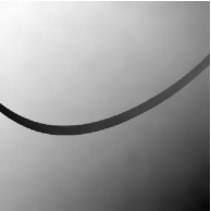
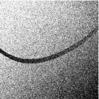
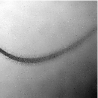
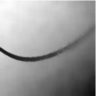
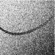
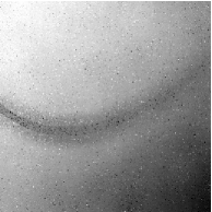
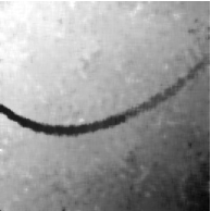
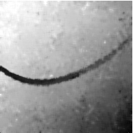
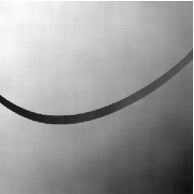
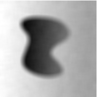
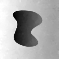
As a simple model of thin feature, consider an image $f$ in the cartoon family, but where $\Omega$ is a thin $d_{0}$-dimensional surface of thickness $a$ — which will vary with $n$. A classical example of this kind of structure is the support bar of the Cameraman’s tripod, see Figure 1(g). An example of function from this class is illustrated by the Swoosh image, see Figure 1(c).

Definition 3 (Thin feature function class).

$$\mathcal{F}^{\rm thin}(\alpha,C_{0},d_{0},a):=\left\{f\in\mathcal{F}(\alpha,C_{0}):\Omega=\{x=(x^{\prime},z):\operatorname{dist}(z,\phi(x^{\prime}))<a\}\right\},$$

where $\phi:(0,1)^{d_{0}}\to(0,1)^{d-d_{0}}$ is $C_{0}$-Lipschitz.

We may similarly define a class of regular pattern functions which themselves may not be smooth, but which occur repeatedly across the image domain. This structure would be difficult to exploit with, say, wavelet-based methods that fail to take advantage of image redundancy. However, empirical evidence suggests that non-local adaptive kernels can perform quite well on these images. A classical example of this type of image structure is the striped scarf in the Barbara image. The following is a class where $\Omega$ is made of the disjoint union of translates of a smaller region $\Omega_{0}$ of diameter of order $a$ — which will vary with $n$.

Definition 4 (Regular pattern function class).

$$\mathcal{F}^{\rm pattern}(\alpha,C_{0},a):=\left\{f\in\mathcal{F}(\alpha,C_{0}):\Omega=(0,1)^{d}\cap\bigcup_{v\in a\mathbb{Z}^{d}}(\Xi+v)\right\},$$

where $\Xi\subset(0,a)^{d}$ is any set. Note that the union above is disjoint.

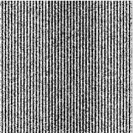
An example of function from this class is illustrated by the Stripes image in Figure 1(d).

3 Background on kernel methods for denoising

We now describe NLM and other related methods. The story starts with kernel smoothing (i.e., linear filtering). Though this age-old method (with a proper choice of kernel) is essentially optimal when the image does not have discontinuities, its performance suffers dramatically in the presence of edges, which it tends to blur. YF, and more generally NLM, attempt to choose the kernel adaptively so as to avoid averaging over the discontinuity.

The estimates we consider are weighted averages of the pixel values of the form

$$\widehat{f}_{i}=\displaystyle\frac{\sum_{j\in I_{n}^{d}}\,\omega_{i,j}\,y_{j}}{\sum_{j\in I_{n}^{d}}\,\omega_{i,j}}\,.$$ (9)

The various methods that we study in this paper differ only in the choice of weights $\omega_{i,j}$. Adaptation to higher order of smoothness is often accomplished by a local polynomial regression (LPR) [17, 20]. The local polynomial estimator of degree $r$ and weights $(\omega_{i,j})$ is

$$\begin{cases}&\widehat{f}_{i}=\widehat{a}^{(i)}_{0}\\ &\widehat{\mathbf{a}}^{(i)}=\displaystyle\mathop{\mathrm{arg\,min}}_{\mathbf{a}}\sum_{j\in I_{n}^{d}}\omega_{i,j}\left(y_{j}-\sum_{0\leq|s|\leq r}a_{s}\,(x_{j}-x_{i})^{s}\right)^{2},\end{cases}$$ (10)

where $x^{s}:=x_{1}^{s_{1}}\cdots x_{d}^{s_{d}},$ for $x=(x_{1},\dots,x_{d})\in\mathbb{R}^{d}$ and $s=(s_{1},\dots,s_{d})\in\mathbb{R}^{d}$, and the minimization in (10) is over $\mathbf{a}=(a_{s}:0\leq|s|\leq r)\in\mathbb{R}^{q}$ where $q={r+d\choose d}$. Note that, in fact, (10) leads to an estimator of the form (9) with different weights (e.g., a smoother kernel) [57, p. 34]. We assume throughout that the polynomial degree $r$ is sufficiently large to take full advantage of the smoothness of $f$. Specifically, if $f\in\mathcal{F}^{\rm cartoon}(\alpha,C_{0})$, we assume that $r\geq\lfloor\alpha\rfloor$. When the number of nonzero weights in (10) is not enough to determine $\widehat{f}_{i}$ uniquely, we define $\widehat{f}_{i}$ as $y_{i}$, namely, we do not apply any smoothing. Alternatively, one could decrease the degree of the polynomial regression until the fit is well-defined, but this is not important in our setting.

Since we know that $f$ takes values in $[0,1]$, we clip $\widehat{f}$ so that it also takes values in $[0,1]$. This clipping does not increase the MSE.

3.1 Linear filtering (LF)

This method can be traced back in the statistics literature to the work of Nadaraya [38] and Watson [60] (cf. [20] for details on kernel methods). In this context the choice of the similarity between two pixels is only controlled by spatial proximity:

$$\omega_{i,j}=K_{h}(x_{i},x_{j})\,,$$ (11)

where $K_{h}(x,x^{\prime})=K(\frac{x}{h},\frac{x^{\prime}}{h})$ for a kernel function $K$ and a bandwidth $h>0$, which is independent of the location in the nonadaptive (classical) version. Common choices include the Gaussian kernel, but we focus on the box kernel

$$K_{h}(x,x^{\prime}) =\mathds{1}{\{\|x-x^{\prime}\|_{\infty}\leq h\}}.$$ (12)

3.2 Yaroslavsky’s filter (YF)

YF was introduced by Yaroslavsky [62] and independently by Lee [28], and more modern variants such as SUSAN [48] and Bilateral filtering [55]. Here, similarity between pixels is based on their spatial distance and on the relative proximity of image intensity at these pixels. This translates into choosing weights in (9) of the form

$$\omega_{i,j}=K_{h}(x_{j},x_{j})\ L_{h_{y}}(y_{i},y_{j})\,,$$ (13)

where $K,L$ are kernels and $h,h_{y}$ the associated bandwidths. $(K,h)$ control the spatial proximity while $(L,h_{y})$ control the photometric proximity. As in classical kernel smoothing, $h$ plays the role of spatial bandwidth, while $h_{y}$ is a photometric bandwidth. In this work we only consider the simple version using the box kernel:

$$K_{h_{y}}(y,y^{\prime}) =\mathds{1}{\{|y-y^{\prime}|\leq h_{y}\}}.$$ (14)

3.3 Non-Local Means (NLM) and patch-based methods

NLM and other patch-based methods generalize the idea of including the photometric proximity in the kernel. In [6], the distance between two pixels is solely measured in terms of the discrepancy between patches surrounding the pixels considered. Though spatial proximity was already introduced in [6], it was only mentioned as a numerical parameter to solve a computational issue. However, later works (cf. [44, 64]) have shown that spatial proximity can improve NLM performance. We consider NLM with spatial proximity, which includes the non-local version, the two being identical when $h$ is sufficiently large.

A generic description is the following. Let $h_{\textsf{P}}>0$ and let $\textsf{P}_{i}$ (leaving $h_{\textsf{P}}$ implicit) be the hypercube of width $h_{\textsf{P}}$ centered at $x_{i}$, i.e.,

$$\textsf{P}_{i}=x_{i}+\left[-\frac{h_{\textsf{P}}}{2},\frac{h_{\textsf{P}}}{2}\right]^{d}=\left\{x:\|x-x_{i}\|_{\infty}\leq\frac{h_{\textsf{P}}}{2}\right\}.$$ (15)

Such a patch corresponds to a pixel patch of width $[h_{\textsf{P}}n]+1$ in the digital image (where $[a]$ denotes the largest integer not exceeding $a\in\mathbb{R}$). Let ${\mathbf{y}_{\textsf{P}_{i}}}=(y_{j}:x_{j}\in\textsf{P}_{i})$ be the vector of pixel values over the patch centered at $x_{i}$. With this notation, the weights used in NLM are:

$$\omega_{i,j}=K_{h}(x_{i},x_{j})\ L_{h_{y}}\left({\mathbf{y}_{\textsf{P}_{i}}},{\mathbf{y}_{\textsf{P}_{j}}}\right)\,,$$ (16)

where $K,L$ are kernel functions and $h,h_{y}$ are bandwidths, as before. One classical choice of $L_{h_{y}}$ (which we consider in our theoretical results) is

$$L_{h_{y}}\left({\mathbf{y}_{\textsf{P}_{i}}},{\mathbf{y}_{\textsf{P}_{j}}}\right)=\mathds{1}\{\|{\mathbf{y}_{\textsf{P}_{i}}}-{\mathbf{y}_{\textsf{P}_{j}}}\|_{2}\leq h_{y}\}.$$ (17)

The photometric similarity is based on the Euclidean distance between the patches (as vectors) around the pixels. We refer to this as “classical” or Euclidean NLM (or just NLM).

Computing $L_{h_{y}}$ can be computationally intensive for large $h_{\textsf{P}}$. To address this, some authors have considered projecting ${\mathbf{y}_{\textsf{P}_{i}}}$ onto a low-dimensional subspace and using this projection to compute an approximation of $L_{h_{y}}({\mathbf{y}_{\textsf{P}_{i}}},{\mathbf{y}_{\textsf{P}_{j}}})$. This introduces an interesting trade-off between computational complexity and accuracy which is examined in [4, 54]. In this paper, we consider a $1$-dimensional projection introduced in [31] where patches are simply compared via their means alone, resulting in a photometric kernel of the form

$$L_{h_{y}}\left({\mathbf{y}_{\textsf{P}_{i}}},{\mathbf{y}_{\textsf{P}_{j}}}\right)=\overline{L}_{h_{y}}\left({\overline{y}_{\textsf{P}_{i}}},{\overline{y}_{\textsf{P}_{j}}}\right),\quad{\overline{y}_{\textsf{P}_{i}}}:={\rm Ave}({\mathbf{y}_{\textsf{P}_{i}}}).$$ (18)

We refer to this method as NLM-average. For our theoretical results, we consider the kernel

$$\overline{L}_{h_{y}}\left({\overline{y}_{\textsf{P}_{i}}},{\overline{y}_{\textsf{P}_{j}}}\right)=\mathds{1}\{|{\overline{y}_{\textsf{P}_{i}}}-{\overline{y}_{\textsf{P}_{j}}}|\leq h_{y}\}.$$ (19)

In our analysis, Euclidean NLM (17) and NLM-average (19) behave similarly, except for the regular pattern model, where the former is generally superior. In practice, however, we note a difference. In smooth regions, the average in (19) has little bias and little variance, making it significantly more robust to noise than the Euclidean distance (17). Near edges or patterns, however, the bias of the average in (19) can outweigh the variance, making Euclidean NLM (17) superior. This insight is supported by our experimental results in Section 6.

The spatial bandwidth $h$ is typically larger than the patch width $h_{\textsf{P}}$. Common sizes used in practice are $21\times 21$ kernel windows (also referred to as the searching zone) and $7\times 7$ patches (in pixel units). Common kernels are the box-kernel for $K$ and the Gaussian kernel for $L$. Though we assume box kernels for both, our results extend readily to other kernel functions.

4 Oracle inequalities and minimax results for cartoon images

We analyze the performance of the kernel-based methods described in Section 3 within the mathematical framework detailed in Section 2. Qualitatively speaking, our theoretical results are congruent with what is observed in practice; see our experiments in Section 6.

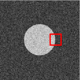
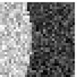
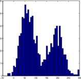
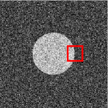
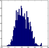
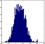
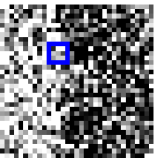
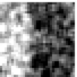
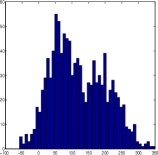
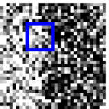
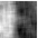
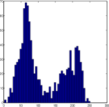
Indeed, we show that LF blurs edges, which is in fact well-known both in theory and practice. YF performs well when the JNR is large, and poorly otherwise. This filter relies on a clear gap between the pixel values on either side of the discontinuity: when the JNR is large, there is indeed a gap, which ceases to exist when the JNR is of order 1 (cf. Figure 2). The latter situation is where NLM shines. Indeed, patches of size larger than one pixel gather more information about the area surrounding the pixel, which NLM (implicitly) uses to assess whether two pixels are on the same size of the discontinuity. For example, comparing patches in Figure 3, we see that the means of sufficiently large patches allow us to estimate reliably whether each center pixel is in $\Omega$ or not, even with an JNR of order 1.

Fig. 2: On the left column are cartoon images with increasing levels of noise (rows are with $JNR=4,2,1$ from top to bottom). A searching zone is displayed in red, for a pixel near the discontinuity. The middle column is a close-up of the searching zone, while the right one provides histograms of pixel values within it.

Fig. 3: We use again the image from Figure 2, last row (JNR=1). The noisy image is displayed in the first column, with kernel supports. The second column is the result of the local (box) kernel averaging using support of width 1, 3 and 7 from top to bottom. The last column provides histograms of the filtered pixels

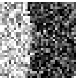
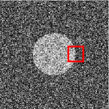
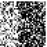
In what follows, we focus on the LPR variants described in (10) to avoid a systematic bias that conventional weighted average variants suffer from. It is well-known that this bias appears near the boundary of the image, though this can be corrected with a proper extension of the image. More importantly, this bias arises also near the discontinuity. Note that enforcing the spatial windows to have the same (symmetric) shape puts a real constraint on the resulting performance of the algorithm, as discussed in Section 4.3. The choice of kernel $K$ for LPR variants (10) is unimportant for standard kernel regression as long as it satisfies some basic properties. (For example, in [17, Th. 3.1], the kernel does not impact the error rate except for a multiplicative constant.) Less is known about the impact of the choice of $L$. In this paper, we consider box kernels for both spatial and photometric components, namely (12), (17) or (19).

To obtain our bounds, we minimize the error with respect to the bandwidth parameter $h$, effectively striking a good balance between the bias and variance in (3). Indeed, the larger the bandwidth, the larger the bias and the smaller the variance. The issue with kernel smoothing — whether in the form of weighted average (9) or LPR (10) — is that it suffers from a substantial bias when the smoothing window (those points where the weights are equal to one) includes points from the “other side” of the discontinuity. At the same time, the window cannot be too small, for otherwise the variance will be overwhelming.

4.1 Linear kernel smoothing blurs edges

It is well-known that LF blurs discontinuities. This comes from the fact that the window size is fixed — the same at all pixels — so points near and points far from the discontinuity are treated in the same way. This lack of adaptivity leads to a substantial MSE. How does that statement translate into a mathematical result within our framework? The following is proved in [2] for $d\leq 2$, though the result (at least the upper bound) is probably older; see also [27]. We provide a proof for LPR in Section 8.

Theorem 4.1.

Let $\widehat{\mathbf{f}}_{h}^{\rm LF}$ denote the linear estimator, in the form of either local average (9) or LPR (10), with weights as in (11). We have

$$\inf_{h}\mathcal{R}_{n}(\widehat{\mathbf{f}}_{h}^{\rm LF},\mathcal{F}^{\rm cartoon}(\alpha,C_{0}))\asymp\mathcal{R}^{\rm LF}:=(\sigma^{2}/n^{d})^{1/(d+1)},$$

and the optimal choice of bandwidth is $h\asymp h^{\rm LF}:=(\sigma^{2}/n^{d})^{1/(d+1)}$.

Note that the bound does not depend on the regularity $\alpha\geq 1$ of the function $f$. As apparent in the proof, this is because LF blurs edges: to strike a good bias-variance trade-off, the smoothing window cannot be too small, transforming sharp edges into ramps. The resulting bias is then larger than the bias over the smooth regions, which is where $\alpha$ appears.

4.2 Oracle kernel

What can we hope to achieve with adaptive kernel methods? Statisticians have used the notion of an oracle to answer this question [13, 21, 57]. We saw that what limits linear filtering is a large bias near the discontinuity, due to the mixing of pixels from both sides. What if we had access to an oracle that would identify for us the foreground and the background?

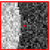
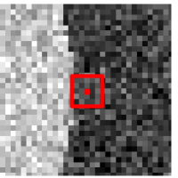
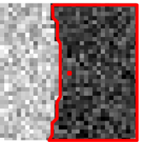
The membership oracle tells us which sample points belong to $\Omega$ or to $\Omega^{c}$. With access to this oracle, we simply process the smooth pieces, $f_{\Omega}$ and $f_{\Omega^{c}}$, separately. By doing so we achieve the minimax rate for the class $\mathcal{H}_{d}(\alpha,C_{0})$: the information this oracle provides is sufficient to do as well as if there were no discontinuity. This is illustrated in Figure 4 (best viewed in color).

(a) Kernel smoothing

(b) Bandwidth oracle

(c) Membership oracle

Fig. 4: The kernel supports for the linear filter, the bandwidth oracle and the membership oracle

Theorem 4.2.

Let $\widehat{\mathbf{f}}_{h}^{\rm MO}$ denote LPR estimator (10) with weights as in (11) when $x_{i}$ and $x_{j}$ belong to the same side of the discontinuity, and set to zero otherwise. We have

$$\inf_{h}\mathcal{R}_{n}(\widehat{\mathbf{f}}_{h}^{\rm MO},\mathcal{F}^{\rm cartoon}(\alpha,C_{0}))\asymp\mathcal{R}^{\rm MO}:=(\sigma^{2}/n^{d})^{2\alpha/(d+2\alpha)},$$

and the optimal choice of bandwidth is $h\asymp h^{\rm MO}:=(\sigma^{2}/n^{d})^{1/(d+2\alpha)}$.

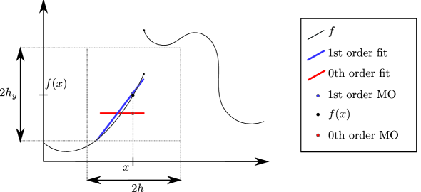
The lower bound is a well-known minimax bound [27, Theorem 5.1.2, p. 133]. If we consider a class of piecewise polynomial functions, then this oracle estimator, without spatial proximity (i.e., $h=\infty$), achieves the parametric rate of $\sigma^{2}/n^{d}$. It is worth noting that LPR plays a crucial role here. Indeed, the window around a point near the discontinuity — comprised of all points belonging to the same side of the discontinuity — will be irregularly shaped. For instance, imagine a point on a linear surface adjacent to the discontinuity. For a symmetric window (sufficiently small not to include the discontinuity), the linear variations around the pixel of interest will average out and we can accurately estimate the pixel value. For an asymmetric window caused by the discontinuity, the linear variations will not average out, inducing a small bias and leading to a higher risk of order $(\sigma^{2}/n^{d})^{3/(d+3)}$ when $\alpha\geq 3/2$. This phenomenon can be observed in practice and is illustrated in Figure 5.

Fig. 5: Membership oracles of order 0 and 1 on a non-noisy 1D signal. Note how the bias is reduced by going to the order 1.

Note that the oracle only has to provide the membership information locally, within the searching window. The insight we get from this is that we only need to know over which pixel values to average to attain the same error rate as we would without discontinuities. This is exactly what adaptive kernel methods [29], including patch-based methods, PDE methods [39, 1, 19] and graph diffusion methods [52, 47] aim at doing.

4.3 Variable bandwidth kernel methods

These methods [37, 50, 22, 23, 24], including Lepski’s method [29] and variants [40, 41], choose the bandwidth adaptively at every location, the goal being to avoid smoothing over discontinuities and to adapt to the regularity of the signal when unknown. Wavelet shrinkage methods are often thought to perform some sort of variable-bandwidth kernel smoothing [13]. Clearly, we cannot do better than if we knew the discontinuity, meaning if we had access to the membership oracle. In that case, at each point we would choose the bandwidth equal to its distance to the discontinuity (BO below stands for bandwidth oracle). See Figure 4 for a comparison of the MO and BO spatial supports.

Theorem 4.3.

Let $\widehat{\mathbf{f}}_{h}^{\rm BO}$ denote LPR estimator (10) with weights chosen as in (11) when $\|x_{i}-x_{j}\|_{\infty}<\operatorname{dist}(x,\partial\Omega):=\displaystyle\inf_{y\in\partial\Omega}\|x-y\|_{\infty}$, and set to zero otherwise. We have

$$\inf_{h}\mathcal{R}_{n}(\widehat{\mathbf{f}}_{h}^{\rm BO},\mathcal{F}^{\rm cartoon}(\alpha,C_{0}))\asymp\mathcal{R}^{\rm BO}:=(A_{n}\sigma^{2}/n)\vee(\sigma^{2}/n^{d})^{2\alpha/(d+2\alpha)},$$

where $A_{n}=\log n$ when $d=1$ and $A_{n}=1$ when $d\geq 2$, for an optimal choice of maximal bandwidth $h\asymp h^{\rm MO}$.

Note that BO achieves the error rate of MO only when $d=1$, when $d=2$ and $\alpha=1$, or when $d\geq 2$ and $\sigma^{2}=O(n^{-2\alpha(1-1/d)+1})$, which is polynomially small when $d=2$ and $\alpha>1$ or when $d\geq 3$. Thus in general, BO is substantially weaker than MO. That said, BO achieves the minimax rate established in [56] when $\sigma$ is fixed.

4.4 Yaroslavsky’s filter is oracle-optimal under low noise

As the practitioner knows, YF can be quite good on natural images. In fact, it can dramatically outperforms the linear filter and compares favorably with methods such as wavelet thresholding, particularly when the noise level is small. We substantiate this empirical evidence with a theoretical study of its performance, showing it achieves MO bound in such situations (i.e., when $\sigma$ is small).

Assume that for a fixed cumulative distribution function $F$, the noise satisfies the following

$$\mathbb{P}(|\varepsilon_{i}|\leq t)\geq F(t/\sigma),\ \forall t,\ \forall i\in I_{n}^{d},$$ (20)

The following result states that YF achieves a performance comparable to that of MO if $\sigma$ is small. We only require that the noise distribution in (20) has quickly decaying tails.

Theorem 4.4.

Let $\widehat{\mathbf{f}}_{h,h_{y}}^{\rm YF}$ denote the LPR estimator (10) with Yaroslavsky’s weights (13). Suppose that, for some constants $C,b>0$, (20) holds with $1-F(t)\leq C\exp(-(t/C)^{b})$ for $t$ large enough. Then there is another constant $C^{\prime}>0$ such that, if $\sigma\leq(C^{\prime}\log n)^{-1/b}$,

$$\inf_{h,h_{y}}\mathcal{R}_{n}(\widehat{\mathbf{f}}_{h,h_{y}}^{\rm YF},\mathcal{F}^{\rm cartoon}(\alpha,C_{0}))\leq(1+o(1))\mathcal{R}^{\rm MO},$$

where an optimal choice of bandwidths is $h\asymp h^{\rm MO}$ and $h_{y}\asymp 1$.

Gaussian noise satisfies the requirements of Theorem 4.4 with $C=\sqrt{2}$ and $b=2$, resulting in the constraint $\sigma=O(1/\sqrt{\log n})$, which is quite mild. This explains why YF tends to perform well in practice, at least for low noise level.

This excellent performance hinges on the fact that the photometric kernel is able to mimic the membership oracle when the noise level is small. When the noise level is of order 1 or larger, this is no longer true, as illustrated in Figure 2. There, we clearly see that in a window containing points from both $\Omega$ and its complement, the pixel values are mixed in the histogram if the noise level is too large, making a clear separation impossible. We formally argue this point after the proof of Theorem 4.4 in Section 8.2.4.

It is worth noting that the proof helps clarify exactly the artifacts encountered in practice by the YF for strong noise (cf. Figure 10). Indeed, the output often looks like the original scene contaminated by something like “salt and pepper” noise. As mentioned in the proof, this is because the YF does not alter pixels with extreme values.

4.5 Performance analysis for Non-Local Means

In the previous section we established that YF performs as well as MO when the noise level is small, while it is useless otherwise. A natural strategy consists of, first, reducing the noise level by averaging and, then, applying YF. This is almost exactly what NLM-average does. We precisely quantify the MSE performance of both NLM-average and Euclidean NLM in this section. Note that we state our results for i.i.d. Gaussian noise for simplicity, though they are valid for many other distribution families such as uniform and double-exponential.

Theorem 4.5.

Let $\widehat{\mathbf{f}}_{h,h_{y}}^{\rm NLM}$ denote LPR estimator (10) with NLM weights (16) and photometric kernel either Euclidean (17) or Average (19). If the noise conditions of Theorem 4.4 hold, then

$$\inf_{h,h_{y}}\mathcal{R}_{n}(\widehat{\mathbf{f}}_{h,h_{y}}^{\rm NLM},\mathcal{F}^{\rm cartoon}(\alpha,C_{0}))\leq(1+o(1))\mathcal{R}^{\rm MO},$$

where $h_{\textsf{P}}=1/n$. Otherwise, assuming $\sigma$ is bounded away from 0, we have

$$\inf_{h,h_{y}}\mathcal{R}_{n}(\widehat{\mathbf{f}}_{h,h_{y}}^{\rm NLM},\mathcal{F}^{\rm cartoon}(\alpha,C_{0}))\preceq\mathcal{R}^{\rm NLM}:=(B_{n}/n)\vee(\sigma^{2}/n^{d})^{2\alpha/(d+2\alpha)},$$

where $B_{n}:=(\sigma^{4}\log n)^{1/d}$ (Euclidean) or $:=(\sigma^{2}\log n)^{1/d}$ (Average), and an optimal choice of bandwidths is $h\asymp h^{\rm MO}$, $h_{y}\asymp h_{y}^{\rm NLM}:=\sigma^{3}\sqrt{\log n}$ (Euclidean) or $:=(2C_{0})^{-d}\mu/2$ (Average), and $h_{\textsf{P}}\asymp h_{\textsf{P}}^{\rm NLM}:=B_{n}/n$.

In other words, if the low-noise conditions of Theorem 4.4 hold, then the optimal patch size is a single pixel, and the NLM is exactly YF and we achieve the YF performance bound. There is an elbow in the performance bound, since once the optimal patch size exceeds a single pixel, estimation errors within a patch sidelength of the boundary impact the performance.

There is a strong correspondence between this bound and the BO bound in Theorem 4.3. If $\sigma$ is fixed, $\mathcal{R}^{\rm NLM}\asymp\mathcal{R}^{\rm BO}$ for $d=1$ and $\mathcal{R}^{\rm NLM}\asymp(\log n)^{1/d}\mathcal{R}^{\rm BO}$ for $d\geq 2$, therefore $\mathcal{R}^{\rm BO}$ is the minimax rate [56] and NLM is minimax optimal up to a logarithmic factor.

Note that our bandwidth $h$ is not infinite as in [34]. There, the authors use an infinite window for searching for matching patches: this is optimal in their setting because they consider piecewise constant images. In our setting, images are piecewise smooth, and a smaller bandwidth can not only help us reduce the risk of our estimate, but also lead to more computationally efficient estimation algorithms.

5 Performance analysis for thin features and textures

In the cartoon model of Section 2 with JNR of order 1, the performance of NLM is comparable to that of variable bandwidth kernel smoothing, and actually that of wavelets as well [26, 42]. In natural images, however, NLM can perform substantially better. We explain this by the fact that the cartoon model we considered so far, though useful as a benchmark, does not account for features common in natural images, particularly, very thin regions a few pixels wide and regular textures.

Below, we do as if the image contained regions of cartoon type and regions with thin features and/or texture, and keep the same bandwidths that we found to be optimal in the cartoon model in the previous results.

5.1 Thin features

Both YF and NLM achieve a good performance on thin features. We focus on sample points within the feature and focus on the interesting case where the thickness is of smaller order of magnitude than the bandwidth $h$.

Theorem 5.1.

Consider $f\in\mathcal{F}^{\rm thin}(\alpha,C_{0},d_{0},a)$ with band $\Omega$; assume all parameters are fixed except $a\geq 4/n$ and $a\rightarrow 0$ as $n\rightarrow\infty$ . In terms of point-wise risk (3) at $x_{i}\in\Omega$, we have:

1. The linear filter with bandwidth $h^{\rm LF}$ has risk of order 1 if $a=o(h^{\rm LF})$.

2. BO with maximal bandwidth $h^{\rm MO}$ has a point-wise risk of order $a^{2\alpha}\vee\sigma^{2}(na)^{-d}$, if $\operatorname{dist}(x_{i},\Omega^{c})\geq a/C$ for some $C>3$, if $na\to\infty$.

3. MO with bandwidth $h^{\rm MO}$ has risk of order $(h^{\rm MO}/a)^{d-d_{0}}\mathcal{R}^{\rm MO}$ if $a=o(h^{\rm MO})$.

4. The latter is true of YF with bandwidths $h^{\rm MO},h_{y}\asymp 1$, if the noise satisfies the conditions of Theorem 4.4.

5. This is also the case of NLM (Euclidean or Average) with bandwidths $h=h^{\rm MO},h_{y}=h_{y}^{\rm NLM}$, and patch size $h_{\textsf{P}}=h_{\textsf{P}}^{\rm NLM}$, if $\operatorname{dist}(x_{i},\Omega^{c})\geq h_{\textsf{P}}^{\rm NLM}$.

In view of this result, we can say that linear filtering essentially erases the feature. In contrast, YF still performs very well (relative to the MO) under low noise, and NLM performs well in this case and for higher noise settings. Note that when $h_{\textsf{P}}^{\rm NLM}=o(a)$, the bound above holds for most points within the thin features. Though not stated here, we found that NLM is able to handle such bands under special circumstances — when $d\geq 3$ and the band is straight.

5.2 Regular patterns and textures

We consider very general patterns where YF will do as well as in the cartoon model, situations where most other methods are essentially useless. Euclidean NLM performs well too, under additional assumptions on the pattern.

Proposition 5.1.

Consider $f\in\mathcal{F}^{\rm pattern}(\alpha,C_{0},a)$ with all parameters are fixed except for $a$, which satisfies $a=o(h^{\rm MO})$. Let $N_{\Omega}:=\#\{i:x_{i}\in\Omega\}$ and $N_{\Omega^{c}}$ is defined similarly. If $N_{\Omega}\vee N_{\Omega^{c}}\leq C(N_{\Omega}\wedge N_{\Omega^{c}})$ and $na\geq(r+1)(2C+2)$, with $C>1$ fixed, we have the following:

1. MO with $h=h^{\rm MO}$ achieves an MSE of order $\mathcal{R}^{\rm MO}$.

2. The latter is true of YF with bandwidths $h^{\rm MO},h_{y}\asymp 1$, if the noise satisfies the conditions of Theorem 4.4.

3. Suppose in addition that for every $x_{i}\in\Omega$ and $x_{j}\in\Omega^{c}$,

   $$\|\mathds{1}(\textsf{P}_{i}\cap\Omega)-\mathds{1}(\textsf{P}_{j}\cap\Omega)\|_{2}^{2}\geq(\sigma^{2}\log n)/C^{\prime},$$ (21)

   for some $C^{\prime}>1$ fixed. Then (Euclidean) NLM with bandwidths $h=h^{\rm MO},h_{y}=h_{y}^{\rm NLM}$ and patch size $h_{\textsf{P}}^{\rm NLM}$, achieves an MSE of order $(na)^{d}\,\mathcal{R}^{\rm MO}$.

The condition (21) essentially means that any two patches, where on is centered in the foreground and the other is centered in the background, must be sufficiently distinct – and the necessary degree of distinction increases with the noise level. For instance, (21) is satisfied by such patterns as a chessboard or stripes. A regular pattern in a real image (e.g., Barbara’s blouse) is often referred to as texture, and NLM is able to effectively denoise such patterns under some regularity conditions. For random models of textures, such as Markov random fields, we do not expect NLM to do well unless the pattern is not very random. The reason is that few patches are close in Euclidean distance to a given patch.

6 Experiments

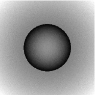
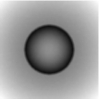
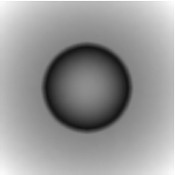
In this section we provide numerical results for images with $d=2$, whose pixel intensities are between $0$ and $255$. In our experiments, the noise is Gaussian with standard deviation $\sigma\in\{5,20,50,100\}$ (Note that this corresponds, for normalized images in $[0,1]$ to noise with $\sigma\in\{5/255,10/255,50/255,100/255\}$).

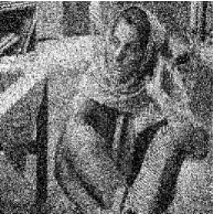
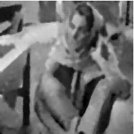
On both toy and classical images, we have compared the behavior of the following methods: linear filtering (LF), Yaroslavsky’s filter (YF), Euclidean NLM (NLM), average non-local means (NLM-average) and the membership oracle (MO). In all cases we have implemented LPR version of the methods for the orders $r\in\{0,1,2\}$. Note that, as expected, for linear filtering LPR of order 0 and 1 are exactly identical because the support of the kernel is symmetric. However, for other methods the symmetry of the support is no longer guaranteed and the estimators differ. The higher order LPR versions are computed by solving the linear system in (26). A small numerical constant ($10^{-8}$) is added to the diagonal elements of $\mathbf{X}^{T}\mathbf{X}$ so that inverting this matrix is always a well conditioned problem.

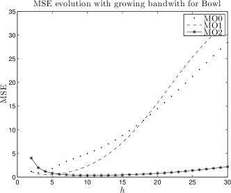
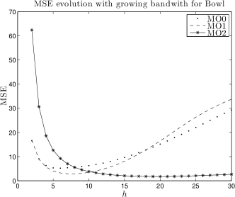
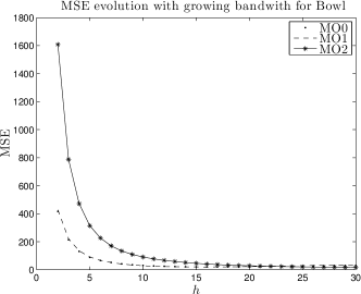
For fair comparisons we have used the same box kernel with every method. The patch size is $7\times 7$ (i.e., $h_{\textsf{P}}=7$). It is kept fixed for all the methods. For the spatial bandwidth $h$ we have chosen to use the values obtained by considering the best $h$ (in term of MSE) for the MO, on the Bowl image. Thus, we use for each noise level $\sigma\in\{5,20,50,100\}$ and polynomial order $r\in\{0,1,2\}$ an $h$ optimized on Bowl. The values are provided by the MSE optimization in Figure 6 and summarized in Tab. 6. The photometric bandwidth $h_{y}$ is chosen by hand, and differs from method to method: $\sqrt{10}\sigma$ (YF), $0.29\sigma$ (NLM-average), $13.1\sigma$ (NLM), $30$ (MO). It is to be noted that the parameters are given for comparison in between methods, we do not claim those are the best parameters for all applications.

(a) $\sigma=5$

(b) $\sigma=20$

(c) $\sigma=20$

(d) $\sigma=100$

Fig. 6: MSE with respect to $h$ for the image Bowl, with noise level $\sigma\in\{5,20,50,100\}$.

	$\sigma=5$	$\sigma=20$	$\sigma=50$	$\sigma=100$
$r=0$	7	13	23	35
$r=1$	9	17	25	33
$r=2$	23	41	59	61

Table 1: Spatial bandwidth $h$ used in practice obtained by minimizing the MSE of the MO on Bowl (cf. Figure 6).

In practice, $h$ needs to increase with $r$ to ensure that the LPR is stable. Note that there are $q={r+d\choose d}$ polynomial coefficients in each search window. If we apply the rule of thumb of 10 observations per unknown parameter, the search window needs to include about $10q$ pixels. This is illustrated in Figure 6, where we see the best $h$ increasing with $r$.

Since for natural (not cartoon-like) images MO is irrelevant, we have used a modified YF oracle instead. This oracle has access to the original image to compute the weights as in (11), and then performs LPR on the noisy pixel values with these weights. For piecewise constant images, this coincides exactly with MO as soon as the bandwidth is large enough.

The experiments conducted show that LF is always outperformed in practice by YF, NLM and NLM-average. For low noise level ($\sigma=5$), the YF with $r=2$ outperforms the other methods (cf. Figure 11 and Table 6). However, in the presence of strong noise the NLM and the NLM-average are the clear winners on most images. Interestingly, and may be surprisingly the NLM-average  can even improve on the NLM for very strong noise, even for natural images. On the other hand, one can see that the NLM-average mimics the behavior of LF for textured images with strong noise (cf. Figure 14), due to the fact that different sides of periodic features are averaged together. This limitation is particularly obvious for the Stripe image 14.

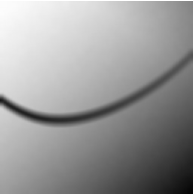
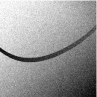
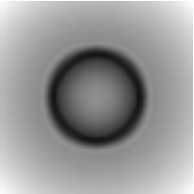
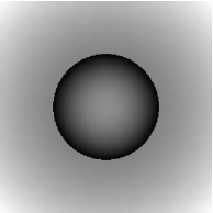
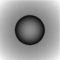
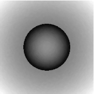
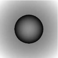
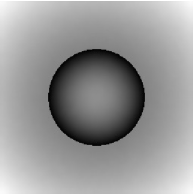
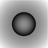
The influence of the degree $r$ of the LPR depends on the nature of the image being denoised (e.g., natural vs. cartoon images). In practice it remains unclear how this parameter should be tuned. Figure 7, Figure 8, Figure 9, and Figure 10 demonstrate the importance of the jump parameter $\mu$ in practice. On the left end of the Swoosh, the jump is larger and we reconstruct it accurately across all noise levels. On the right end, the jump is smaller and the performance degrades with $\sigma$, exactly as predicted by our theory.

The MATLAB codes are available on the authors’ webpages to reproduce those results.

Table 2: MSE comparisons of the denoising methods considered for LPR of order 0, 1 and 2. The compared methods are the Linear Filter (LF), the Yaroslavsky Filter (YF), the NLM-average (NLM-Av.), the classical NLM and the Membership Oracle (MO). Results are averaged over 5 Gaussian noise replicas.

(a) Noisy, MSE = 2.50e+01

(b) LF0, MSE = 4.03e+01

(c) LF1, MSE = 5.55e+01

(d) LF2, MSE = 8.29e+01

(e) YF0, MSE = 1.69e+00

(f) YF1, MSE = 1.31e+00

(g) YF2, MSE = 1.19e+00

(h) NLM-Av.0, MSE = 2.56e+00

(i) NLM-Av.1, MSE = 1.90e+00

(j) NLM-Av.2, MSE = 1.75e+00

(k) NLM0, MSE = 1.54e+00

(l) NLM1, MSE = 1.36e+00

(m) NLM2, MSE = 1.37e+00

(n) MO0, MSE = 1.79e+00

(o) MO1, MSE = 1.26e+00

(p) MO2, MSE = 1.31e+00

Fig. 7: Toy thin feature image (Swoosh) corrupted Gaussian noise with $\sigma=5$.

(a) Noisy, MSE = 3.99e+02

(b) LF0, MSE = 9.18e+01

(c) LF1, MSE = 1.35e+02

(d) LF2, MSE = 2.09e+02

(e) YF0, MSE = 1.71e+01

(f) YF1, MSE = 2.08e+01

(g) YF2, MSE = 2.49e+01

(h) NLM-Av.0, MSE = 9.86e+00

(i) NLM-Av.1, MSE = 8.37e+00

(j) NLM-Av.2, MSE = 7.87e+00

(k) NLM0, MSE = 6.19e+00

(l) NLM1, MSE = 6.00e+00

(m) NLM2, MSE = 4.53e+00

(n) MO0, MSE = 4.54e+00

(o) MO1, MSE = 3.39e+00

(p) MO2, MSE = 2.85e+00

Fig. 8: Toy thin feature image (Swoosh) corrupted Gaussian noise with $\sigma=20$.

(a) Noisy, MSE = 2.50e+03

(b) LF0, MSE = 2.13e+02

(c) LF1, MSE = 2.35e+02

(d) LF2, MSE = 2.91e+02

(e) YF0, MSE = 1.38e+02

(f) YF1, MSE = 1.56e+02

(g) YF2, MSE = 1.78e+02

(h) NLM-Av.0, MSE = 3.11e+01

(i) NLM-Av.1, MSE = 2.91e+01

(j) NLM-Av.2, MSE = 2.64e+01

(k) NLM0, MSE = 3.54e+01

(l) NLM1, MSE = 4.25e+01

(m) NLM2, MSE = 4.35e+01

(n) MO0, MSE = 8.61e+00

(o) MO1, MSE = 8.32e+00

(p) MO2, MSE = 6.40e+00

Fig. 9: Toy thin feature image (Swoosh) corrupted Gaussian noise with $\sigma=50$.

(a) Noisy, MSE = 9.98e+03

(b) LF0, MSE = 3.22e+02

(c) LF1, MSE = 3.11e+02

(d) LF2, MSE = 3.07e+02

(e) YF0, MSE = 3.67e+02

(f) YF1, MSE = 3.58e+02

(g) YF2, MSE = 3.54e+02

(h) NLM-Av.0, MSE = 8.55e+01

(i) NLM-Av.1, MSE = 8.27e+01

(j) NLM-Av.2, MSE = 8.11e+01

(k) NLM0, MSE = 1.78e+02

(l) NLM1, MSE = 1.78e+02

(m) NLM2, MSE = 1.68e+02

(n) MO0, MSE = 1.51e+01

(o) MO1, MSE = 1.82e+01

(p) MO2, MSE = 1.86e+01

Fig. 10: Toy thin feature image (Swoosh) corrupted Gaussian noise with $\sigma=100$.

(a) Noisy, MSE = 2.50e+01

(b) LF0, MSE = 5.76e+01

(c) LF1, MSE = 7.40e+01

(d) LF2, MSE = 1.05e+02

(e) YF0, MSE = 1.71e+00

(f) YF1, MSE = 9.88e-01

(g) YF2, MSE = 8.74e-01

(h) NLM-Av.0, MSE = 3.41e+00

(i) NLM-Av.1, MSE = 2.50e+00

(j) NLM-Av.2, MSE = 2.15e+00

(k) NLM0, MSE = 1.67e+00

(l) NLM1, MSE = 1.60e+00

(m) NLM2, MSE = 1.50e+00

(n) MO0, MSE = 9.56e-01

(o) MO1, MSE = 5.01e-01

(p) MO2, MSE = 3.48e-01

Fig. 11: Toy cartoon image (Bowl) corrupted Gaussian noise with $\sigma=5$.

(a) Noisy, MSE = 3.99e+02

(b) LF0, MSE = 7.78e+01

(c) LF1, MSE = 1.04e+02

(d) LF2, MSE = 1.40e+02

(e) YF0, MSE = 1.53e+01

(f) YF1, MSE = 1.80e+01

(g) YF2, MSE = 1.90e+01

(h) NLM-Av.0, MSE = 7.55e+00

(i) NLM-Av.1, MSE = 6.62e+00

(j) NLM-Av.2, MSE = 5.10e+00

(k) NLM0, MSE = 5.86e+00

(l) NLM1, MSE = 5.83e+00

(m) NLM2, MSE = 4.92e+00

(n) MO0, MSE = 4.12e+00

(o) MO1, MSE = 3.03e+00

(p) MO2, MSE = 2.37e+00

Fig. 12: Toy cartoon image (Blob) corrupted Gaussian noise with $\sigma=20$.

(a) Noisy, MSE = 2.50e+03

(b) LF0, MSE = 9.00e+02

(c) LF1, MSE = 9.55e+02

(d) LF2, MSE = 1.15e+03

(e) YF0, MSE = 6.53e+02

(f) YF1, MSE = 6.99e+02

(g) YF2, MSE = 8.10e+02

(h) NLM-Av.0, MSE = 4.20e+02

(i) NLM-Av.1, MSE = 4.17e+02

(j) NLM-Av.2, MSE = 4.26e+02

(k) NLM0, MSE = 4.50e+02

(l) NLM1, MSE = 4.76e+02

(m) NLM2, MSE = 4.96e+02

(n) MO0, MSE = 5.28e+01

(o) MO1, MSE = 5.86e+01

(p) MO2, MSE = 5.18e+01

Fig. 13: Barbara image corrupted Gaussian noise with $\sigma=50$.

(a) Noisy, MSE = 9.98e+03

(b) LF0, MSE = 1.71e+04

(c) LF1, MSE = 1.78e+04

(d) LF2, MSE = 1.71e+04

(e) YF0, MSE = 8.91e+03

(f) YF1, MSE = 9.26e+03

(g) YF2, MSE = 8.87e+03

(h) NLM-Av.0, MSE = 7.39e+03

(i) NLM-Av.1, MSE = 7.51e+03

(j) NLM-Av.2, MSE = 7.25e+03

(k) NLM0, MSE = 2.42e+02

(l) NLM1, MSE = 2.10e+02

(m) NLM2, MSE = 2.33e+02

(n) MO0, MSE = 2.11e+01

(o) MO1, MSE = 2.37e+01

(p) MO2, MSE = 2.28e+01

Fig. 14: Toy texture image (Stripes) corrupted Gaussian noise with $\sigma=100$.

7 Discussion

The theoretical results of the preceding sections are summarized in Table 3.

Image class	Method	Bound
$\mathcal{F}^{\rm cartoon}$	MO	$\mathcal{R}_{n}\asymp\mathcal{R}^{\rm MO}:=(\sigma^{2}/n^{d})^{2\alpha/(d+2\alpha)}$
	LF	$\mathcal{R}_{n}\asymp(\sigma^{2}/n^{d})^{1/(d+1)}$
	YF	$\mathcal{R}_{n}\leq(1+o(1))\mathcal{R}^{\rm MO}$ (for low noise)
	NLM	$\mathcal{R}_{n}\preceq\begin{cases}(1+o(1))\mathcal{R}^{\rm MO}&\mbox{ for low noise }\\ [(\sigma^{4}\log n)^{1/d}/n]\vee\mathcal{R}^{\rm MO}&\mbox{ otherwise}\end{cases}$
	NLM-Av.	$\mathcal{R}_{n}\preceq\begin{cases}(1+o(1))\mathcal{R}^{\rm MO}&\mbox{ for low noise }\\ [(\sigma^{2}\log n)^{1/d}/n]\vee\mathcal{R}^{\rm MO}&\mbox{ otherwise}\end{cases}$
$\mathcal{F}^{\rm pattern}$	MO	$\mathcal{R}_{n}\asymp\mathcal{R}^{\rm MO}$
	LF	$\mathcal{R}_{n}\asymp 1$
	YF	$\mathcal{R}_{n}\preceq\mathcal{R}^{\rm MO}$ (for low noise)
	NLM	$\mathcal{R}_{n}\preceq\begin{cases}(1+o(1))\mathcal{R}^{\rm MO}&\mbox{ for low noise }\\ [(na)^{d}\mathcal{R}^{\rm MO}&\mbox{ for ``distinct'' patterns}\end{cases}$
$\mathcal{F}^{\rm thin}$	MO	$\mathbb{E}(\widehat{f}_{i}-f_{i})^{2}\asymp(h^{\rm MO}/a)^{d-d_{0}}\mathcal{R}^{\rm MO}$
	LF	$\mathbb{E}(\widehat{f}_{i}-f_{i})^{2}\asymp 1$
	YF	$\mathbb{E}(\widehat{f}_{i}-f_{i})^{2}\preceq(h^{\rm MO}/a)^{d-d_{0}}\mathcal{R}^{\rm MO}$ (for low noise)
	NLM	$\mathbb{E}(\widehat{f}_{i}-f_{i})^{2}\preceq(h^{\rm MO}/a)^{d-d_{0}}\mathcal{R}^{\rm MO}$
	NLM-Av.	$\mathbb{E}(\widehat{f}_{i}-f_{i})^{2}\preceq(h^{\rm MO}/a)^{d-d_{0}}\mathcal{R}^{\rm MO}$

Table 3: Summary of results

As described in the Introduction, the bounds described in this paper and in the independent work [34, 33] address fundamental performance limits of NLM and related photometric image filtering methods. These methods have an established history of strong empirical performance on natural images, but until now little was known about how these methods performed asymptotically, especially with respect to related methods based on computational harmonic analysis (e.g., wavelet or curvelet denoising).

Both our bounds and the bounds in [34] suggest that NLM has some limitations for piecewise smooth images when the noise is not small (i.e., when YF cannot perform effectively). When the noise is small, we note that YF is a special case of NLM with a patch size of one pixel, and the performance of NLM hinges upon our ability to measure the similarity of two patches based on noisy observations. In low noise, this similarity can already be estimated quite accurately with a single pixel patch. In stronger noise, the similarity measured through larger patches is more robust to noise — but larger patches also introduce some bias. This results in an elbow in the performance bounds for NLM. Recent empirical results suggest that these limitations can be mitigated by adapting the kernel shape [53], the patch shape [12], or spatial bandwidth $h$ [26]; a theoretical understanding of this kind of adaptation remains an open problem.

There are several distinctions between our work and the closely related work in [34] that bear mentioning. First, we consider the cartoon model, where the functions are piecewise Hölder smooth images with a discontinuity set corresponding to a Lipschitz mapping of the unit ball, while Maleki et al. [34] consider the horizon edge model, where the functions are piecewise constant with a discontinuity set corresponding to the graph of a Lipschitz function. Though they actually consider smoother edges, their analysis reduces to the case of Lipschitz smoothness. We consider images in arbitrary dimension — showing that NLM behaves differently when $d\geq 3$ — while Maleki et al. consider the case of 2D images ($d=2$). Because they consider functions that are piecewise constant, they use the weighted average version (9) without spatial localization (i.e., $h=\infty$). Because we focus on smooth — not necessarily constant — regions, we need to localize both YF and NLM. Applying the more complex LPR (10) enables YF to adapt to the degree of regularity in each smooth region. We note that Maleki et al. [34] do not consider the case of low noise and simply show that YF achieves the same performance as LF — which is also our conclusion in strong noise.

Moreover to simplify the analysis, Maleki et al. consider a slightly modified version of NLM and derive lower bounds for oracle versions of YF and NLM. The lower bounds for NLM were also challenging for us and we only provide heuristics. We mention that our results imply that the simpler NLM-average achieves the same performance as NLM in the horizon model.

Let us also comment on the work of Tsybakov [56]. This paper suggests and analyzes (within the cartoon model) a method very similar to NLM-average, based on medians rather than means. The method is based on non-overlapping patches. This allows the method to be applicable in situations where the noise distribution is heavy-tailed. (We were not aware of this work when we prepared our paper.)

Our analysis of NLM for image classes with thin features or regular patterns is also a significant novel aspect of our work. Though we expect wavelets are near-optimal for cartoon images when the discontinuity is Lipschitz, NLM has a significant empirical advantage over wavelets for certain kinds of repeating textures. We develop a model for images with these features, and note that it does not approach cartoon or horizon model asymptotically. For this image class, we demonstrate that NLM performs as well as it does for the cartoon class.

The current bounds are based on ideal bandwidths which depend on the unknown smoothness parameter $\alpha$. Thus we have demonstrated that the adaptive filtering techniques considered adapt to the discontinuity $\Omega$, but not to $\alpha$. We anticipate that adaptivity to $\alpha$ is indeed possible and leave that analysis for future work.

We note that NLM is not the current state-of-the-art image denoising method in common use. More evolved patch-based methods utilize sparse representations of patches, adaptive kernel bandwidths, and adaptive patch shapes (cf. [9, 10, 32, 11, 49, 53]). While these aspects are not considered in our analysis, the theoretical insights provided by this paper may potentially lead to an improved understanding of a broad class of patch-based image denoising methods and subsequently better algorithms (cf. [46] for possible directions).

8 Proofs

In this section, $C,C_{1},C_{2},\dots$ denote finite positive constants that do not change with $n$ and whose actual value may change with each appearance.

8.1 Preliminary results

We first gather some basic results.

8.1.1 Some analysis

Functions in $\mathcal{H}_{d}(\alpha,C_{0})$ are uniformly well-approximated locally by polynomials of degree $\lfloor\alpha\rfloor$, specifically their Taylor expansions. For $g\in\mathcal{H}_{d}(\alpha,C_{0})$ and $x\in[0,1]^{d}$, the Taylor expansion of $g$ at $x$ of degree $t\in\mathbb{N}$ is defined as follows: T^r_x g(x’) = ∑_—s— ≤t g^(s)(x)  ∏_i=1^d (xi’ - xi)sisi!.

Lemma 8.1.

For any $g\in\mathcal{H}_{d}(\alpha,C_{0})$, —g(x’) - T^⌊α⌋_x g (x’)— ≤c_α C_0 ∥x’ - x∥_∞^α,  ∀x, x’ ∈[0,1]^d, where

$$c_{\alpha}:=\sum_{s\in\mathbb{N}^{d}:|s|=\lfloor\alpha\rfloor}\frac{1}{s_{1}!\cdots s_{d}!}.$$

Proof.

Though this sort of result is well-known, we provide a proof for completeness. A Taylor approximation of degree $\lfloor\alpha\rfloor$ gives: g(x’) =T^⌊α⌋_x g (x’) + ∑_—s— = ⌊α⌋ (g^(s)(z) - g^(s)(x))  ∏_i=1^d (xi’ - xi)sisi!, for some $z$ on the segment joining $x$ and $x^{\prime}$. Hence, —g(x’) - T^⌊α⌋_x g (x’)— ≤c_α ∥x’ - x∥_∞^⌊α⌋ max_—s— = ⌊α⌋ —g^(s)(z) - g^(s)(x)—. Now apply (5) and the fact that $\|z-x\|_{\infty}\leq\|x^{\prime}-x\|_{\infty}$ to get —g^(s)(z) - g^(s)(x)— ≤C_0 ∥x’ - x∥_∞^α- ⌊α⌋,  ∀s ∈N^d, —s— = ⌊α⌋.                                                                                                                                                                                                                              ∎

8.1.2 Some geometry

For a measurable set $A\subset\mathbb{R}^{d}$,

$$\rho(A):=\inf_{h\in(0,1)}\inf_{x\in A}\sup\left\{\frac{{\rm Vol}(B(y,s))}{{\rm Vol}(B(x,h))}:B(y,s)\subset B(x,h)\cap A\right\}.$$ (22)

The quantity $\rho(A)$ provides some measure of how irregular the boundary of $A$ is. The following lemma bounds $\rho$ from below for sets whose boundary is sufficiently regular.

Lemma 8.2.

Let $\phi:\mathbb{R}^{d}\to\mathbb{R}^{d}$ be injective, with $\phi$ and $\phi^{-1}$ both $C$-Lipschitz. Then for $\Omega=\phi(B(0,1))$ and $\rho$ defined in (22), we have $\min(\rho(\Omega),\rho(\Omega^{c}))\geq(2C)^{-d}$.

Proof.

Fix $x\in\Omega$ and $h>0$. Since $\phi$ is Lipschitz with constant $C$, we have $\phi(B(\phi^{-1}(x),h/C))\subset B(x,h)$. Note that $z:=\phi^{-1}(x)\in B(0,1)$ and, by the triangle inequality, $B(z,h/C)\cap B(0,1)\supset B(z^{\prime},t)$, where $z^{\prime}:=(1-h/(2C))z$ and $t:=h/(2C)$. Because $\phi^{-1}$ is $C$-Lipschitz, we have $\phi^{-1}(B(\phi(z^{\prime}),t/C))\subset B(z^{\prime},t)$, so that

$$B(y,s)\subset\phi(B(z^{\prime},t))\subset\phi(B(z,h/C)\cap B(0,1))\subset B(x,h)\cap\Omega,$$

where $y:=\phi(z^{\prime})$ and $s:=t/C$. We obtain a lower bound for $\Omega^{c}$ in a similar way. ∎

Next is a result on the number of sample points within a certain distance of a subset. Let $\mathcal{X}_{n^{d}}$ be the set of sample points, that is, $\mathcal{X}_{n^{d}}=\{x_{i}:i\in I_{n}^{d}\}$.

Lemma 8.3.

For any subset $A\subset(0,1)^{d}$ of the form $A=B(A^{\prime},\eta)$ for some $A^{\prime}\subset(0,1)^{d}$ and $4/n\leq\eta\leq 1$, 8^-d n^d Vol(A) ≤—A ∩X_n^d— ≤4^d n^d Vol(A).

Proof.

Let $z_{1},\dots,z_{k}\in(0,1)^{d}$ be a maximal $\eta$-packing for $A^{\prime}$ (i.e., the balls $B(z_{j},\eta/2)$ for $j=1,\dots,k$ are disjoint and included in $A^{\prime}\subset A$, and for any $z\in A^{\prime}$, there is $j$ such that $z\in B(z_{j},\eta)$). By the triangle inequality, we have ⋃_j=1,…,k B(z_j, η/2) ⊂A ⊂⋃_j=1,…,k B(z_j, 2 η). On the one hand, taking volumes on all sides, we get $k\eta^{d}\leq{\rm Vol}(A)\leq k2^{d}(2\eta)^{d}$, since the unit ($\|\cdot\|_{\infty}$) ball has volume $2^{d}$. This turns into $4^{-d}{\rm Vol}(A)\leq k\eta^{d}\leq{\rm Vol}(A)$. On the other hand, counting sample points on all sides, using the fact that

$$\eta^{d}n^{d}\leq|B(z,\eta)\cap\mathcal{X}_{n^{d}}|\leq(2\eta)^{d}n^{d},\quad\forall z\in(0,1)^{d},\ \forall\eta\in(2/n,1),$$

we get k (η/2)^d n^d ≤∑_j=1^k —B(z_j, η/2) ∩X_n^d— ≤—A ∩X_n^d— ≤∑_j=1^k —B(z_j, 2 η) ∩X_n^d— ≤k (4η)^d n^d. Combining these, we get the desired result. ∎

Lemma 8.4.

Suppose $1\leq d_{0}\leq d$ are integers and let $\phi:\mathbb{R}^{d_{0}}\to\mathbb{R}^{d}$ be injective, with $\phi$ and $\phi^{-1}$ (on the range of $\phi$) both $C$-Lipschitz with $C\geq 1$. Then there is another constant $C^{\prime}>1$ such that, for $A:=\phi((0,a)^{d_{0}})$ and $h\in(0,1)$,

$$\frac{1}{C^{\prime}}a^{d_{0}}h^{d-d_{0}}\leq{\rm Vol}(B(A,h))\leq C^{\prime}a^{d_{0}}h^{d-d_{0}}.$$

Consequently, if $\phi:\mathbb{R}^{d}\to\mathbb{R}^{d}$ is as above and $A:=\phi(\partial B(0,1))$, the result holds with $d-d_{0}=1$.

Proof.

We first observe that, for any $z\in\mathbb{R}^{d_{0}}$ and $h>0$, since $\phi$ is $C$-Lipschitz,

$$\phi(B(z,h))\subset B(\phi(z),Ch).$$ (23)

Now, let $z_{1},\dots,z_{m}$ denote a maximal $h$-packing of $(0,a)^{d_{0}}$. Note that $m\asymp(a/h)^{d_{0}}$ when $h\leq 1$. By definition $\|z_{i}-z_{j}\|\geq h$, so that $\|\phi(z_{i})-\phi(z_{j})\|\geq h/C$ since $\phi^{-1}$ is $C$-Lipschitz with $C\geq 1$. Hence,

$$\bigsqcup_{i=1,\dots,k}B(\phi(z_{i}),h/C)\subset B(A,h/C)\subset B(A,h),$$

implying

$$\sum_{i=1}^{m}{\rm Vol}(B(\phi(z_{i}),h/C))\leq{\rm Vol}(B(A,h)).$$

We then conclude by the fact that $\sum_{i=1}^{m}{\rm Vol}(B(\phi(z_{i}),h/C))\asymp mh^{d}\asymp a^{d_{0}}h^{d-d_{0}}$. For the upper bound, we use the fact that $(0,a)^{d_{0}}\subset\cup_{i=1,\dots,k}B(z_{i},h)$, so that

$$A\subset\bigcup_{i=1,\dots,k}\phi(B(z_{i},h))\subset\bigcup_{i=1,\dots,k}B(\phi(z_{i}),Ch),$$

by (23). Hence, using the triangle inequality,

$${\rm Vol}(B(A,h))\leq\sum_{i=1}^{m}{\rm Vol}(B(\phi(z_{i}),Ch+h))\asymp mh^{d}\asymp a^{d_{0}}h^{d-d_{0}}.$$

For the second part, we use the fact that $\partial B(0,1)=\cup_{\ell}\phi_{\ell}((0,1)^{d-1})$ for a finite set of functions $\phi_{\ell}$ satisfying the requirements and the fact that the composition $\phi\circ\phi_{\ell}$ is also Lipschitz. ∎

8.1.3 Some statistics

We establish here some bounds on the point-wise MSE (3) of LPR (10). We mention that much finer results exist in dimension $d=1$ for the case where the underlying function $f$ is smooth; see [17] and references therein.

Lemma 8.5 (Variance).

For any sufficiently large constant $C>0$, depending only on $d,r,$ the following is true. Consider the LPR estimator of the form (10), with weights $\omega_{i,j}\in\{0,1\}$. Assume that $B_{i}^{\rm in}\subset A_{i}:=\{j:\omega_{i,j}=1\}\subset B_{i,h}:=\{j:x_{j}\in B(x_{i},h)\}$, for some discrete ball $B_{i}^{\rm in}$ satisfying $|B_{i}^{\rm in}|\geq|B_{i,h}|/C$ for some constant $C$.

$$\frac{1}{C}\sigma^{2}(nh)^{-d}\leq\operatorname{Var}(\widehat{f}_{i})\leq C\sigma^{2}(nh)^{-d}.$$ (24)

Proof.

We assume without loss of generality that $x_{i}=0$ and drop the subscript $i$ for simplicity. Below $C$ denotes a generic constant that may change with each appearance. Let

$$q=\sum_{s=0}^{r}{s+d-1\choose d-1}={r+d\choose d},$$ (25)

which is the number of monomials in $d$ variables of degree $r$ or less. Let $\mathbf{X}$ denote the $|A|\times q$ matrix with coefficients $(x_{j}^{s}:j\in A,|s|\leq r)$. By definition of the local polynomial estimator (10) and the usual least squares formula, we have

$$\widehat{f}=\mathbf{e}^{T}(\mathbf{X}^{T}\mathbf{X})^{-1}\mathbf{X}^{T}\mathbf{y},$$ (26)

where $\mathbf{e}=(1,0,\dots,0)\in\mathbb{R}^{q}$ and $\mathbf{y}:=(y_{j}:j\in A)$ (assuming that $\mathbf{X}$ is full-rank, which we prove further down). In particular,

$$\operatorname{Var}(\widehat{f})=\sigma^{2}\mathbf{e}^{T}(\mathbf{X}^{T}\mathbf{X})^{-1}\mathbf{e},$$

since $y_{j}=f(x_{j})+\varepsilon_{j}$, with the noise $(\varepsilon_{j})$ being uncorrelated and having identical variance $\sigma^{2}$.

Let $z_{j}=x_{j}/h$ and $\mathbf{Z}=(z_{j}^{s}:j\in A,|s|\leq r)$, and also let $\mathbf{H}=\mathop{\operator@font diag}\nolimits(h^{|s|},|s|\leq r)$, so that $\mathbf{X}=\mathbf{Z}\mathbf{H}$, leading to

$$\operatorname{Var}(\widehat{f})=\sigma^{2}\mathbf{e}^{T}\mathbf{H}^{-1}(\mathbf{Z}^{T}\mathbf{Z})^{-1}\mathbf{H}^{-1}\mathbf{e}=\sigma^{2}\mathbf{e}^{T}(\mathbf{Z}^{T}\mathbf{Z})^{-1}\mathbf{e},$$ (27)

since $\mathbf{H}^{-1}\mathbf{e}=\mathbf{e}$. This is because $\mathbf{H}$ is an invertible diagonal matrix with first element equal to 1. The reason we work with $\mathbf{Z}$ instead of $\mathbf{X}$ is that, under the conditions assumed here, $z_{j}\in[-1,1]^{d}$ (because $j\in A$) and $(nh)^{-d}\mathbf{Z}^{T}\mathbf{Z}$ is bounded from above and below in terms of its spectrum. Indeed, define matrices $\mathbf{Z}_{1}=(z_{j}^{s}:j\in B^{\rm in},|s|\leq r)$, $\mathbf{Z}_{2}=(z_{j}^{s}:j\in A\setminus B^{\rm in},|s|\leq r)$, $\mathbf{Z}_{3}=(z_{j}^{s}:j\in B_{h},|s|\leq r)$ and $\mathbf{Z}_{4}=(z_{j}^{s}:j\in B_{h}\setminus A,|s|\leq r)$. Let $\prec$ denote the ordering for positive semi-definite matrices. Since

$$\mathbf{Z}_{1}^{T}\mathbf{Z}_{1}\prec\mathbf{Z}_{1}^{T}\mathbf{Z}_{1}+\mathbf{Z}_{2}^{T}\mathbf{Z}_{2}=\mathbf{Z}^{T}\mathbf{Z}=\mathbf{Z}_{3}^{T}\mathbf{Z}_{3}-\mathbf{Z}_{4}^{T}\mathbf{Z}_{4}\prec\mathbf{Z}_{3}^{T}\mathbf{Z}_{3},$$

it suffices that we focus on proving a lower bound on the spectrum of $\mathbf{Z}_{1}^{T}\mathbf{Z}_{1}$ and upper bound on the spectrum of $\mathbf{Z}_{3}^{T}\mathbf{Z}_{3}$. Consider therefore the case where $A$ itself is a discrete ball, say $A=\{j:x_{j}\in B(x,ah)\}$, where $a\in(C^{-1/d},1)$ by assumption. Let $z=x/h$. First, assume that $a$ and $h$ remain fixed. Then for $s,t\in\mathbb{N}^{d}$ such that $|s|\vee|t|\leq r$, we have

$$\frac{1}{(nh)^{d}}(\mathbf{Z}^{T}\mathbf{Z})_{st}=(nh)^{-d}\sum_{j\in A}z_{j}^{s+t}\to M_{st}:=\int_{B(z,a)}u^{s+t}du,\quad\text{ when }nh\to\infty,$$ (28)

recognizing a Riemann sum on the LHS. So, if $\mathbf{M}=(M_{st}:|s|\vee|t|\leq r)$, we have the convergence $(nh)^{-d}\ \mathbf{Z}^{T}\mathbf{Z}\to\mathbf{M},$ when $nh\to\infty$. $\mathbf{M}$ is a well-defined positive semi-definite matrix since its elements are bounded by 1 — because $B(z,a)\subset B(0,1)$ — so we only need to show that it is positive uniformly over $a\in(C^{-1/d},1)$. Let $\lambda_{z,a}$ denote the smallest eigenvalue of $\mathbf{M}$ with integral over $B(z,a)$, with $z\in B(0,1)$ and $a\in(C^{-1/d},1)$. We want to show that $\lambda_{z,a}$ is bounded away from 0. Suppose this is not the case, that there are sequences $(z_{m},a_{m})$ such that $\lambda_{z_{m},a_{m}}\to 0$ as $m\to\infty$. By compacity, we may assume that $(z_{m},a_{m})\to(z_{\infty},a_{\infty})\in\overline{B(0,1)}\times[C^{-1/d},1]$. Then $\lambda_{z_{\infty},a_{\infty}}=0$, by continuity. Let $\mathbf{M}_{\infty}$ be the associated matrix. Then there is $b_{\infty}\in\mathbb{R}^{q}$ nonzero such that

$$0=b_{\infty}^{T}\mathbf{M}_{\infty}b_{\infty}=\int_{B(z_{\infty},a_{\infty})}\sum_{s,t}b_{\infty_{s}}b_{\infty,t}u^{s+t}du=\int_{B(z_{\infty},a_{\infty})}\Big{(}\sum_{s}b_{\infty,s}u^{s}\Big{)}^{2}du,$$

where the sums are over $s\in\mathbb{N}^{d}$ such that $|s|\leq r$. This leads to a contradiction since the polynomial in the second integral cannot be zero on a nonempty ball.

So far, we assumed that $a$ and $z$ were fixed. Assume this is not the case. The upper bound on the largest eigenvalue of $\mathbf{Z}^{T}\mathbf{Z}$ is bounded in the exact same way, using the fact that $\|z_{j}\|\leq 1$. For the lower bound we still have that

$$\liminf\ (nh)^{-d}\sum_{j\in A}z_{j}^{s+t}\geq\inf_{z^{\prime},a^{\prime}}\int_{B(z^{\prime},a^{\prime})}u^{s+t},du$$

where the inf is over $z^{\prime}$ and $a^{\prime}$ such that $a^{\prime}\in(C^{-1/d},1)$ and $B(z^{\prime},a^{\prime})\subset B(0,1)$. Our arguments apply to the RHS. We conclude that there is $C_{1}\in(0,\infty)$ such that, for $nh$ large enough,

$$\frac{1}{C_{1}}(nh)^{d}\leq\lambda_{\rm min}(\mathbf{Z}^{T}\mathbf{Z})\leq\lambda_{\rm max}(\mathbf{Z}^{T}\mathbf{Z})\leq C_{1}(nh)^{d}.$$ (29)

We then redefine $C$ as $\max(C,C_{1})$ and conclude with (27). ∎

Lemma 8.6 (Bias: Upper Bound).

Assume that $f\in\mathcal{F}^{\rm cartoon}(\alpha,C_{0})$, with foreground $\Omega$, and that the conditions of Lemma 8.5 also hold. If moreover either $A_{i}\subset\Omega$ or $A_{i}\subset\Omega^{c}$, then, for some constant $C>0$, the following inequality holds

$$(\mathbb{E}\widehat{f}_{i}-f_{i})^{2}\leq\min(1,Ch^{2\alpha}).$$ (30)

Proof.

We continue with the notation introduced in the proof of Lemma 8.6. WLOG, assume $A\subset\Omega$. In that case, $f$ is smooth in the window, since $f=f_{\Omega}$. By Lemma 8.1, $f(x_{j})=T_{0}^{\lfloor\alpha\rfloor}f(x_{j})+g(x_{j})$, where $T_{0}^{\lfloor\alpha\rfloor}f$ is a polynomial of degree at most $\lfloor\alpha\rfloor\leq r$, and $|g(x_{j})|\leq c_{\alpha}C_{0}h^{\alpha}$ for all $j\in A$. Now, for a polynomial $p$ of degree at most $r$, let $\mathbf{p}=(p(x_{j}):j\in A)$ so that $\mathbf{p}=\mathbf{X}\mathbf{a}$ for some $\mathbf{a}\in\mathbb{R}^{q}$, and we have

$$\mathbf{e}^{T}(\mathbf{X}^{T}\mathbf{X})^{-1}\mathbf{X}^{T}\mathbf{p}=\mathbf{e}^{T}\mathbf{a}=a_{0}=p(0).$$

With this reproducing formula and the fact that $T_{0}^{\lfloor\alpha\rfloor}f(0)=f(0)$,

$$\mathbb{E}\widehat{f}-f(0)=\mathbf{e}^{T}(\mathbf{X}^{T}\mathbf{X})^{-1}\mathbf{X}^{T}\mathbf{g}=\mathbf{e}^{T}(\mathbf{Z}^{T}\mathbf{Z})^{-1}\mathbf{Z}^{T}\mathbf{g}.$$

Because of (29), we have

$$|\mathbf{e}^{T}(\mathbf{Z}^{T}\mathbf{Z})^{-1}\mathbf{Z}^{T}\mathbf{g}|\leq\frac{\|\mathbf{e}\|_{2}\cdot\|\mathbf{Z}^{T}\mathbf{g}\|_{2}}{\lambda_{\rm min}(\mathbf{Z}^{T}\mathbf{Z})}\leq C_{1}(nh)^{-d}\|\mathbf{Z}^{T}\mathbf{g}\|_{2},$$ (31)

where $C_{1}$ is the constant of Lemma 8.5. But the entries $(\mathbf{Z}^{T}\mathbf{g})_{s}=\sum_{j\in A}g(x_{j})z_{j}^{s}$ are uniformly bounded by $|A|\cdot c_{\alpha}C_{0}h^{\alpha}=O((nh)^{d}h^{\alpha})$, so that the RHS in (31) is of order $O(h^{\alpha})$. This imply that $(\mathbb{E}\widehat{f}-f(0))^{2}\leq C_{2}h^{2\alpha}$ for some constant $C_{2}$, and we conclude by redefining $C$ as $\max(C,C_{1},C_{2})$. ∎

Lemma 8.7 (Bias: Lower Bound).

Let $f={\bf 1}_{\Omega}$, where $\Omega=(0,1/2)\times(0,1)^{d-1}$ and linear filtering (meaning $\omega_{i,j}=1$ if, and only if, $\|x_{i}-x_{j}\|\leq h/2$). Then there is a constant $C>0$ such that, when $\operatorname{dist}(x_{i},\partial\Omega)\leq h/C$, we have

$$(\mathbb{E}\widehat{f}_{i}-f_{i})^{2}\geq 1/C.$$ (32)

Proof.

We continue with the notation introduced in the proof of Lemma 8.6. In particular, we translate everything so that $x_{i}=0$. WLOG, assume that $x_{i}\in\Omega$ and let $\delta=\operatorname{dist}(x_{i},\partial\Omega)$. Let $A_{\Omega}=\{j:x_{j}\in B_{h}\cap\Omega\}$ and define $A_{\Omega^{c}}$ similarly. Using the reproducing formula, we get

$$\mathbb{E}\widehat{f}-f(x_{i})=\mathbf{e}^{T}(\mathbf{Z}^{T}\mathbf{Z})^{-1}\mathbf{Z}^{T}{\bf 1}_{A_{\Omega}}-\mathbf{e}^{T}(\mathbf{Z}^{T}\mathbf{Z})^{-1}\mathbf{Z}^{T}{\bf 1}=-\mathbf{e}^{T}(\mathbf{Z}^{T}\mathbf{Z})^{-1}\mathbf{Z}^{T}{\bf 1}_{A_{\Omega^{c}}}.$$ (33)

Assume that $\delta<h$, in which case $A_{\Omega^{c}}=\{j:x_{j}\in(\delta,h)\times(-h,h)^{d-1}\}$, in which case the RHS in (33) is equal to $-G(\delta/h)$, where

$$G(a):=\mathbf{e}^{T}(\mathbf{Z}^{T}\mathbf{Z})^{-1}\mathbf{Z}^{T}{\bf 1}_{\{j:\,z_{j}\in(a,1)\times(-1,1)^{d-1}\}}.$$

It suffices to show that there is $C>0$ such that $G(a)\geq 1/C$ when $a\leq 1/C$. Assume this is not the case, in which case there is $a_{m}\to 0$ such that $G(a_{m})\to 0$. As in the proof of Lemma 8.6, recognizing Riemann sums we see that, as $m\to\infty$,

$$\frac{1}{(nh)^{d}}\mathbf{Z}^{T}\mathbf{Z}\to\mathbf{M}:=\int_{(-1,1)^{d}}\mathbf{p}(z)\mathbf{p}(z)^{T}dz,\quad\mathbf{p}(z):=(z^{s}:|s|\leq r),$$

and

$$\frac{1}{(nh)^{d}}\mathbf{Z}^{T}{\bf 1}_{\{j:\,z_{j}\in(a,1)\times(-1,1)^{d-1}\}}\to\mathbf{v}:=\int_{(0,1)\times(-1,1)^{d-1}}\mathbf{p}(z)dz.$$

Let

$$\mathbf{u}=\int_{(-1,0)\times(-1,1)^{d-1}}\mathbf{p}(z)dz.$$

We have $\mathbf{u}+\mathbf{v}=\mathbf{M}\cdot{\bf 1}$ (where ${\bf 1}=(1,\dots,1)$), so that $\mathbf{e}^{T}\mathbf{M}^{-1}(\mathbf{u}+\mathbf{v})=1$, and therefore $\mathbf{e}^{T}\mathbf{M}^{-1}\mathbf{v}=1/2$ by symmetry. Hence, $G(a_{m})\to 1/2$, which is a contradiction. ∎

This lemma states a lower bound on the squared bias of linear filtering when $f$ is an indicator function of a half hypercube. The result is actually much more general. Any function $f$ in the cartoon class has a foreground $\Omega$ whose boundary is well-approximated by a hyperplane — since $\partial\Omega$ is Lipschitz — and $f$ is approximately locally piecewise constant ($f$ is smooth on $\Omega$ and $\Omega^{c}$). Hence, near the discontinuity, $f$ resembles the function in Lemma 8.7.

8.1.4 Some probability

The following result asserts that the maximum of $m$ identically distributed random variables with exponentially decaying tails is at most a power of $\log m$.

Lemma 8.8.

Suppose $X_{1},\dots,X_{m}$ are such that for some $a,b,c>0$,

$$\mathbb{P}\left(|X_{r}|>t\right)\leq c\exp(-(t/a)^{b}),\quad\forall t>c,\quad\forall r=1,\dots,m.$$

Then for $m$ sufficiently large,

$$\mathbb{P}\left(\max(|X_{1}|,\dots,|X_{m}|)>a(2\log m)^{1/b}\right)\leq c/m.$$

Proof.

Define $x_{m}=a(2\log m)^{1/b}$. By the union bound,

$$\mathbb{P}\left(\max(|X_{1}|,\dots,|X_{m}|)>x_{m}\right) \leq\mathbb{P}\left(|X_{1}|>x_{m}\right)+\cdots\mathbb{P}\left(|X_{m}|>x_{m}\right)$$

$$\leq mc\exp(-(x_{m}/a)^{b})$$

$$=cm^{-1}\to 0.$$

∎

Lemma 8.9.

For $X_{i}\sim\mathcal{N}(0,\sigma_{i}^{2})$ for $i=1,\dots,m$, and any $C>0$, we have

$$\mathbb{P}\left(\max_{1\leq i\leq m}|X_{i}|>\max_{1\leq i\leq m}\sigma_{i}\sqrt{2C\log m}\right)\leq m^{1-C}.$$

Proof.

Fix $t\geq 1$ and let $\sigma=\max_{1\leq i\leq m}\sigma_{i}$. By the union bound and the fact that $\mathbb{P}\left(\mathcal{N}(0,1)>t\right)\leq\exp(-t^{2}/2)$, we have

$$\mathbb{P}\left(\max_{1\leq i\leq m}|X_{i}|>t\right)\leq\sum_{i=1}^{m}\mathbb{P}\left(|X_{i}|>t\right)\leq\sum_{i=1}^{m}\exp(-t^{2}/(2\sigma_{i}^{2}))\leq m\exp(-t^{2}/(2\sigma^{2})).$$

We then plug in $t=\sigma\sqrt{2C\log m}$. ∎

Lemma 8.10.

Suppose $X_{i}\sim\chi_{k}^{2}$ for $i=1,\dots,m$. There is a constant $C_{1}$ such that, for any $C>C_{1}$, if $k\geq(64/9)C\log(m)$, we have

$$\mathbb{P}\left(\max_{1\leq i\leq m}X_{i}>k+2\sqrt{Ck\log m}\right)\leq m^{1-C/2}$$ (34)

$$\mathbb{P}\left(\min_{1\leq i\leq m}X_{i}<k-2\sqrt{Ck\log m}\right)\leq m^{1-C/2}$$ (35)

Proof.

Let us prove the first inequality. Since the moment generating function of a $\chi_{k}^{2}$ is $t\to(1-2t)^{-k/2}\mathds{1}{(t<1/2)}$, Chernoff’s bound gives

$$\mathbb{P}\left(X_{i}>t\right)\leq\exp\left(-(t-k)/2+(k/2)\log(t/k)\right),\quad\forall t>k.$$

We then use the inequality $\log(1+x)\leq x-x^{2}/2+x^{3}/3$, valid for $x\in(0,1)$ and input $t=k+2\sqrt{Ck\log m}$, to get

$$-(t-k)/2+(k/2)\log(t/k) \leq -(t-k)^{2}/(4k)+(t-k)^{3}/(6k^{2})$$

$$= -C\log m+(4/3)C^{3/2}\sqrt{\log(m)/k}\log m,$$

and bound the second term by $(C/2)\log m$. We then obtain

$$\mathbb{P}\left(X_{i}>t\right)\leq m^{-C/2},$$

and apply the union bound as before. The second inequality is proved in the same way considering that $\log(1-x)\geq-x-x^{2}/2-x^{3}/3$ holds for $x\in(0,1)$. ∎

Lemma 8.11.

Suppose $X_{i}\sim\chi_{k}^{2}(\delta_{i}^{2})$ (non-central chi-square) for $i=1,\dots,m$. There is a constant $C_{1}$ such that, for any $C>C_{1}$, if $k\geq 16C\log(m)$ and $\delta_{\rm min}:=\min_{i}\delta_{i}\geq 2\sqrt{C\log m}$ , we have

$$\mathbb{P}\left(\min_{1\leq i\leq m}X_{i}<\delta_{\rm min}^{2}/4+k-3\sqrt{Ck\log m}\right)\leq 2m^{1-C/2}.$$

Similarly, if $\delta_{\rm max}=\max_{i}\delta_{i}\leq\sqrt{C\log m}$, we have

$$\mathbb{P}\left(\max_{1\leq i\leq m}X_{i}>k+3\sqrt{Ck\log m}\right)\leq m^{1-C/2}.$$

Proof.

First, $X_{i}\equiv(Z_{i}+\delta_{i})^{2}+Y_{i}$, where $Z_{i}\sim\mathcal{N}(0,1)$ and $Y_{i}\sim\chi_{k-1}^{2}$ are i.i.d. Hence,

$$\min_{1\leq i\leq m}X_{i}\geq\min_{1\leq i\leq m}(Z_{i}+\delta_{i})^{2}+\min_{1\leq i\leq m}Y_{i}.$$

Let $E_{i}=\displaystyle\{\max_{1\leq i\leq m}|Z_{i}|\geq\sqrt{C\log m}\}$. By Lemma 8.9, we have

$$\mathbb{P}\left(E_{i}\right)\leq m^{1-C/2}.$$

Let

$$F_{i}=\displaystyle\{\min_{1\leq i\leq m}Y_{i}\leq k-1-2\sqrt{C(k-1)\log m}\}.$$

To control the $Y_{i}$’s, we apply inequality (35) to get

$$\mathbb{P}\left(F_{i}\right)\leq m^{1-C/2}.$$

Under $E_{i}^{c}\cap F_{i}^{c}$, we have $\min_{i}X_{i}\geq\delta^{2}/4+k-3\sqrt{Ck\log m}$ and

$$\mathbb{P}\left(E_{i}^{c}\cap F_{i}^{c}\right)=1-\mathbb{P}\left(E_{i}\cup F_{i}\right)\geq 1-\mathbb{P}\left(E_{i}\right)-\mathbb{P}\left(F_{i}\right)\geq 1-2m^{1-C/2}.$$

This proves the bound on $\min_{i}X_{i}$; arguments for $\max_{i}X_{i}$ are similar and simpler. ∎

8.2 Proofs of the main results

8.2.1 Proof of Theorem 4.1

We start with the upper bound. Fix $f\in\mathcal{F}^{\rm cartoon}(\alpha,C_{0})$ with foreground $\Omega$. Let $Q=\{i:\operatorname{dist}(x_{i},\partial\Omega)\leq h\}$. For $i\in Q$, we use the fact that $|\widehat{f}_{i}-f_{i}|\leq 1$, which implies $\mathbb{E}(\widehat{f}_{i}-f_{i})^{2}\leq 1.$ For $i\notin Q$, from Lemma 8.5 and Lemma 8.6, coupled with the bias-variance decomposition (3), we get

$$\mathbb{E}(\widehat{f}_{i}-f_{i})^{2}\leq C(h^{2\alpha}+\sigma^{2}(nh)^{-d}).$$

Using Lemma 8.3, we have $|Q|\leq 4^{d}n^{d}|B(\partial\Omega,h)|$, while and $|B(\partial\Omega,h)|=O(h)$ by Lemma 8.4 and the fact that $|\partial\Omega|$ is of order 1. Summing over all $i\in I_{n}^{d}$, we get

$${\rm MSE}_{f}(\widehat{f})\leq\frac{n^{d}-|Q|}{n^{d}}\cdot C(h^{2\alpha}+\sigma^{2}(nh)^{-d})+\frac{|Q|}{n^{d}}\cdot C(1+\sigma^{2}(nh)^{-d})\leq C_{1}(h+\sigma^{2}(nh)^{-d}).$$

Minimizing the RHS with respect to $h$ yields the upper bound in Theorem 4.1.

For the lower bound, redefine $Q=\{i:\operatorname{dist}(x_{i},\partial\Omega)\leq h/C_{1}\}$, where $C_{1}$ is the constant of Lemma 8.7. For $i\notin Q$, we use Lemma 8.5 and the bias-variance decomposition (3), to get

$$\mathbb{E}(\widehat{f}_{i}-f_{i})^{2}\geq\frac{1}{C_{2}}\sigma^{2}(nh)^{-d}.$$

For $i\in Q$ we use Lemma 8.7 and the bias-variance decomposition (3), to get

$$\mathbb{E}(\widehat{f}_{i}-f_{i})^{2}\geq\frac{1}{C_{1}},$$

Using Lemma 8.3 again, we have the following lower bound on the MSE (for $n$ large enough),

$${\rm MSE}_{f}(\widehat{f})\geq\frac{n^{d}-|Q|}{n^{d}}\cdot\frac{1}{C_{2}}\sigma^{2}(nh)^{-d}+\frac{|Q|}{n^{d}}\cdot\frac{1}{C_{1}}\geq C_{3}(h+\sigma^{2}(nh)^{-d}).$$

Minimizing the RHS with respect to $h$ leads to the lower bound in Theorem 4.1.

8.2.2 Proof of Theorem 4.2

The proof for the upper bound is the same as that of Theorem 4.1 in smooth regions, leading to an upper bound on the MSE of the form

$${\rm MSE}_{f}(\widehat{f})\leq C(h^{2\alpha}+\sigma^{2}(nh)^{-d}).$$

Then minimizing this quantity over $h$ gives the stated result. The lower bound is a well-known minimax bound [27, Theorem 5.1.2, p. 133].

8.2.3 Proof of Theorem 4.3

Let $\delta(x)=\operatorname{dist}(x,\Omega)$. The proof is similar to that of Theorem 4.2, except that the variance varies by location. The point bias is of order $O(h^{\alpha})$ everywhere, because the smoothing window is of radius at most $h$, with all points in the window being on the same side of the discontinuity. However, the point variance is of order $O(\sigma^{2}\lceil n\delta(x_{i})\rceil^{-d})$, since the window is of radius $\delta(x_{i})$ (immediate consequences of Lemma 8.5).

Let us sum the point variances over all the pixels in the image. The situation is different according to the dimension. We start with $d=1$, so that $\Omega=(a,b)\subset(0,1)$. For $\delta$ small enough, there are exactly four points at distance less than $\delta$ from $\partial\Omega$ (two on each side of the two jump locations). Let’s consider the sample points $x_{i}\in[b,1)$, and let $j$ be such that $x_{j-1}<b\leq x_{j}$. Note that $j=bn(1+o(1))$, and we assume that $b$ is fixed. For $i\in[j,j+nh]$, the variance is bounded by $C\sigma^{2}/(i-j+1)$, while for $i\geq j+nh$ (in the smooth region), the variance is of order $O(\sigma^{2}/(nh))$ as before. Hence, summing over $i\geq j$, the averaged variance in that region is bounded by

$$\frac{C\sigma^{2}}{n-nh-j}\left(\sum_{i=j}^{j+[nh]}\frac{1}{i-j+1}+\frac{n-nh-j}{nh}\right)=O(\frac{\sigma^{2}}{n})\left(\sum_{k=1}^{nh}\frac{1}{k}+1\right)=O(\frac{\sigma^{2}\log(n)}{n}).$$

The same is true for all the other three regions.

When $d\geq 2$, the story is just slightly different. Define $Q_{\ell}=\{i:\delta(x_{i})\leq h2^{-\ell}\}$ and let $\ell_{0}$ be such that $h2^{-\ell_{0}}<2/n\leq h2^{-\ell_{0}+1}$. Stratifying, we have the following bound on the averaged variance

$$\frac{C\sigma^{2}}{n^{d}}\left(\sum_{\ell=0}^{\ell_{0}}\ \sum_{i\in Q_{\ell}\setminus Q_{\ell+1}}(nh2^{-\ell-1})^{-d}+\sum_{i\notin Q_{0}}(nh)^{-d}\right)=\frac{C\sigma^{2}}{n^{d}}\sum_{\ell=0}^{\ell_{0}}\ |Q_{\ell}\setminus Q_{\ell+1}|(nh)^{-d}2^{d(\ell+1)}+\frac{C\sigma^{2}}{(nh)^{d}}.$$

By Lemma 8.3 and Lemma 8.4, we have $|Q_{\ell}\setminus Q_{\ell+1}|\leq|Q_{\ell}|\leq C_{1}n^{d}\cdot h2^{-\ell}$, for some constant $C_{1}$. Hence, the first sum on the RHS of the last equation is bounded by

$$C_{2}\sigma^{2}h(nh)^{-d}\sum_{\ell=0}^{\ell_{0}}2^{(d-1)\ell}\leq C_{3}\sigma^{2}h(nh)^{-d}\cdot 2^{(d-1)\ell_{0}}=O(\sigma^{2}/n).$$

This leads to an upper bound on the MSE of the form

$${\rm MSE}_{f}(\widehat{f})\leq C(h^{2\alpha}+\sigma^{2}A_{n}/n+\sigma^{2}(nh)^{-d}).$$ (36)

Minimizing this quantity over $h$ gives the upper bound stated in Theorem 4.3.

For the lower bound, we know from minimax results underlying the lower bound in Theorem 4.2 that there are functions $f$ in the cartoon class where the bias in the smooth regions is of order at least $h^{\alpha}$. As for the variance, our upper bound for the averaged variance is easily seen to be lower bounded (up to a multiplicative constant). This leads to a lower bound identical to (36) modulo a multiplicative constant, and optimizing it leads to the lower bound in Theorem 4.3. We omit details.

8.2.4 Proof Theorem 4.4

Fix $i\in I_{n}^{d}$ and let $\eta_{i}=\max_{j\in B(i,nh)}|\varepsilon_{j}|$. Then by the union bound and (20),

$$\mathbb{P}(\eta_{i}\geq t)\leq|B(i,nh)|\max_{j\in B(i,nh)}\mathbb{P}(|\varepsilon_{j}|\geq t)\leq(2nh+1)^{d}\,(1-F(t/\sigma))=:p.$$ (37)

Hence, with probability at least $1-p$, the event $E_{i}:=\{\eta_{i}\leq t\}$ holds true. WLOG, assume that $x_{i}\in\Omega$. Since $f_{\Omega}$ is $C_{0}$-Lipschitz, we have $|f(x_{i})-f(x_{j})|=|f_{\Omega}(x_{i})-f_{\Omega}(x_{j})|\leq C_{0}h$ when $x_{j}\in\Omega\cap B(x_{i},h)$, and by the triangle inequality, $|y_{i}-y_{j}|\leq C_{0}h+|\varepsilon_{i}-\varepsilon_{j}|\leq C_{0}h+2t$ under $E_{i}$. Suppose there is $x_{j}\in\Omega^{c}\cap B(x_{i},h)$. In that case, there is $x\in\partial\Omega\cap B(x_{i},h)$ and we have

$$|f(x_{i})-f(x_{j})| \geq |f_{\Omega}(x)-f_{\Omega^{c}}(x)|-|f_{\Omega}(x_{i})-f_{\Omega}(x)|-|f_{\Omega^{c}}(x_{j})-f_{\Omega^{c}}(x)|$$

$$\geq \mu(f)-2C_{0}h\geq 1/C_{0}-2C_{0}h,$$

again by the triangle inequality and the fact that $f_{\Omega^{c}}$ is also $C_{0}$-Lipschitz, this implies that

$$|y_{i}-y_{j}|\geq 1/C_{0}-2C_{0}h-|\varepsilon_{i}-\varepsilon_{j}|\geq 1/C_{0}-2C_{0}h-2t,$$

under $E_{i}$. We see that we need $h_{y}\geq C_{0}h+2t$ to ensure that sample points $x_{j}\in\Omega\cap B(x_{i},h)$ are selected, while we require that $h_{y}<1/C_{0}-2C_{0}h-2t$ so that points $x_{j}\in\Omega^{c}\cap B(x_{i},h)$ are disregarded. These two inequalities are, for example, satisfied when $h_{y}=1/(3C_{0})$ and $t=1/(6C_{0})$, and $h$ sufficiently small — by our assumptions, $h=o(1)$. Assume $h_{y}$ and $t$ are chosen that way. Then, when $E_{i}$ holds, the photometric kernel in YF is able to exactly mimic the MO.

We now turn to bounding the MSE. First, we have

$$\mathbb{E}(\widehat{f}_{i}^{\rm YF}-f_{i})^{2}=\mathbb{E}[(\widehat{f}_{i}^{\rm YF}-f_{i})^{2}\mathds{1}_{\{E_{i}\}}]+\mathbb{E}[(\widehat{f}_{i}^{\rm YF}-f_{i})^{2}\mathds{1}_{\{E_{i}^{c}\}}].$$

Since $\widehat{f}_{i}^{\rm YF}=\widehat{f}_{i}^{\rm MO}$ on $E_{i}$,

$$\mathbb{E}[(\widehat{f}_{i}^{\rm YF}-f_{i})^{2}\mathds{1}_{\{E_{i}\}}]=\mathbb{E}[(\widehat{f}_{i}^{\rm MO}-f_{i})^{2}\mathds{1}_{\{E_{i}\}}]\leq\mathbb{E}(\widehat{f}_{i}^{\rm MO}-f_{i})^{2}.$$

And since $|\widehat{f}_{i}^{\rm YF}-f_{i}|\leq 1$ because of our clipping, we have

$$\mathbb{E}[(\widehat{f}_{i}^{\rm YF}-f_{i})^{2}\mathds{1}_{\{E_{i}^{c}\}}]\leq\mathbb{P}(E_{i}^{c})\leq p.$$

It remains to check that $p$ is negligible compared to MO risk given in Theorem 4.2. Indeed, using the fact that $t\asymp 1$, that $h\leq 1$ and that $\sigma\leq(C^{\prime}\log n)^{-1/b}$, we have

$$p=O(nh)^{d}\exp[-(t/(C\sigma))^{b}]=\exp[(d-t^{b}(C^{\prime}/C^{b}))\log n]=o(\sigma^{2}/n^{d})^{2\alpha/(d+2\alpha)},$$

when $C^{\prime}$ is sufficiently large, implicitly assuming that $\sigma$ is at least a polynomial in $n$, for otherwise the trivial estimator $\widehat{y}=y$ is optimal. This concludes the proof.

When the noise level is not small. Assume $\sigma$ is fixed, for simplicity. Note YF is identical to LF when $h_{y}\to\infty$ sufficiently fast. Assume therefore that $h_{y}\leq h_{0}$ for some fixed $h_{0}<\infty$. We now argue that YF is essentially useless when this is the case. Concretely, assume the reverse of (20), meaning

$$\mathbb{P}(|\varepsilon_{i}|\leq t)\leq F(t/\sigma),\ \forall t,\ \forall i\in I_{n}^{d}.$$ (38)

We show that, when $F(2h_{0}/\sigma)<1$, YF has an overall squared bias (and therefore MSE) of order 1, which is comparable to the trivial estimator $\widehat{f}=y$. In other words, for large noise and relatively small $h_{y}$, YF can perform worse than LF. For example, the bias is at least $h_{0}$ at locations $i$ satisfying $|\varepsilon_{i}|\geq h_{0}+h_{y}$. Indeed, we are averaging over values $y_{j}$ such that $|y_{j}-y_{i}|\leq h_{y}$, so that $|\widehat{f}_{i}-y_{i}|\leq h_{y}$ and therefore $|\widehat{f}_{i}-f_{i}|\geq|\varepsilon_{i}|-|\widehat{f}_{i}-y_{i}|\geq(h_{0}+h_{y})-h_{y}=h_{0}$. Moreover, by (38)

$$\mathbb{P}\left(|\varepsilon_{i}|\geq h_{0}+h_{y}\right)\geq 1-F(2h_{0}/\sigma)>0.$$

Integrating the squared bias over these sample points alone leads to a lower bound of order 1.

8.2.5 Proof of Theorem 4.5

For simplicity, we ignore boundary issues and in particular assume that all patches are of same size, with $m_{\textsf{P}}\asymp(nh_{\textsf{P}})^{d}$ sample points each, and similarly for spatial windows, with $m_{h}\asymp(nh)^{d}$ sample points each.

Upper bound for NLM-average. For $i\in I_{n}^{d}$ such that $\textsf{P}_{i}\cap\partial\Omega\neq\emptyset$, we use the fact that $|\widehat{f}_{i}-f_{i}|\leq 1$ to get

$$\mathbb{E}(\widehat{f}_{i}-f_{i})^{2}\leq 1.$$

Consider $i$ with $\textsf{P}_{i}\cap\partial\Omega=\emptyset$. WLOG, assume $\textsf{P}_{i}\subset\Omega$. Take any $j\in B(i,nh)$. By definition,

$${\overline{y}_{\textsf{P}_{j}}}-{\overline{y}_{\textsf{P}_{i}}}={\overline{f}_{\textsf{P}_{j}}}-{\overline{f}_{\textsf{P}_{i}}}+{\overline{\varepsilon}_{\textsf{P}_{j}}}-{\overline{\varepsilon}_{\textsf{P}_{i}}}.$$ (39)

For the noise part we have

$${\overline{\varepsilon}_{\textsf{P}_{j}}}-{\overline{\varepsilon}_{\textsf{P}_{i}}}\sim\mathcal{N}(0,\sigma^{2}\Delta_{ij}/m_{\textsf{P}}^{2}),$$ (40)

where $\Delta_{ij}$ is the number of sample points in the symmetric difference of $\textsf{P}_{i}$ and $\textsf{P}_{j}$. By Lemma 8.9, we have that

$$\max_{j\in B(x_{i},h)}|{\overline{\varepsilon}_{\textsf{P}_{j}}}-{\overline{\varepsilon}_{\textsf{P}_{i}}}|\leq\zeta:=2\sigma\sqrt{C\log(m_{h})/m_{\textsf{P}}},$$ (41)

with probability at least $1-m_{h}^{1-C}$. In the sequel, we fix $C$ large and denote by $E_{i}$ the event (41). For the signal part, we have the following

$${\overline{f}_{\textsf{P}_{i}}}-{\overline{f}_{\textsf{P}_{j}}} = \frac{1}{m_{\textsf{P}}}\sum_{x_{k}\in\textsf{P}_{i}}f(x_{k})-\frac{1}{m_{\textsf{P}}}\sum_{x_{k}\in\textsf{P}_{j}}f(x_{k})$$

$$= \frac{1}{m_{\textsf{P}}}\sum_{x_{k}\in\textsf{P}_{0}}(f(x_{k}+x_{i})-f(x_{k}+x_{j})),$$

where $\textsf{P}_{0}$ is a generic patch centered at 0. If $x_{j}\in\Omega$ with $\textsf{P}_{j}\subset\Omega$, then, since $f_{\Omega}$ is $C_{0}$-Lipschitz,

$$|{\overline{f}_{\textsf{P}_{i}}}-{\overline{f}_{\textsf{P}_{j}}}| \leq \frac{1}{m_{\textsf{P}}}\sum_{x_{k}\in\textsf{P}_{0}}|f_{\Omega}(x_{k}+x_{i})-f_{\Omega}(x_{k}+x_{j})|$$ (42)

$$\leq C_{0}|x_{i}-x_{j}|\leq C_{0}h.$$

If $x_{j}\in\Omega^{c}$, then there is a point $x\in B(x_{i},h)\cap\partial\Omega$, and we have $f(x_{k})=f_{\Omega}(x)+[f_{\Omega}(x_{k})-f_{\Omega}(x)]$ for $x_{k}\in\Omega$ and $f(x_{k})=f_{\Omega^{c}}(x)+[f_{\Omega^{c}}(x_{k})-f_{\Omega^{c}}(x)]$ for $x_{k}\in\Omega^{c}$, with $|f_{\Omega}(x_{k})-f_{\Omega}(x)|\leq C_{0}h$, $|f_{\Omega^{c}}(x_{k})-f_{\Omega^{c}}(x)|\leq C_{0}h$ and $|f_{\Omega}(x)-f_{\Omega^{c}}(x)|\geq 1/C_{0}$. Hence,

$${\overline{f}_{\textsf{P}_{i}}}-{\overline{f}_{\textsf{P}_{j}}} = \frac{1}{m_{\textsf{P}}}\sum_{x_{k}\in\textsf{P}_{i}}f(x_{k})-\frac{1}{m_{\textsf{P}}}\sum_{x_{k}\in\textsf{P}_{j}}f(x_{k})$$

$$= f_{\Omega}(x)+\frac{1}{m_{\textsf{P}}}\sum_{x_{k}\in\textsf{P}_{i}}[f_{\Omega}(x_{k})-f_{\Omega}(x)]$$

$$-f_{\Omega}(x)\frac{|\textsf{P}_{j}\cap\Omega|}{|\textsf{P}_{j}|}-\frac{1}{m_{\textsf{P}}}\sum_{x_{k}\in\textsf{P}_{j}\cap\Omega}[f_{\Omega}(x_{k})-f_{\Omega}(x)]$$

$$-f_{\Omega^{c}}(x)\frac{|\textsf{P}_{j}\cap\Omega^{c}|}{|\textsf{P}_{j}|}-\frac{1}{m_{\textsf{P}}}\sum_{x_{k}\in\textsf{P}_{j}\cap\Omega^{c}}[f_{\Omega^{c}}(x_{k})-f_{\Omega^{c}}(x)]$$

$$= (f_{\Omega}(x)-f_{\Omega^{c}}(x))\frac{|\textsf{P}_{j}\cap\Omega^{c}|}{|\textsf{P}_{j}|}+R,$$

where $|R|\leq 2C_{0}h$. We now use Lemma 8.2 to bound the fraction above from below by $(2C_{0})^{-d}$, to get

$$|{\overline{f}_{\textsf{P}_{i}}}-{\overline{f}_{\textsf{P}_{j}}}|\geq(2C_{0})^{-d}\mu-2C_{0}h.$$ (43)

Using the decomposition (39), coupled with the triangle inequality and (41), (42) and (43), we see that we need to choose $h_{y}$ such that

$$C_{0}h+\zeta\leq h_{y}<(2C_{0})^{-d}\mu-2C_{0}h-\zeta.$$ (44)

The lower bound is to ensure that all the points $x_{j}\in B(x_{i},h)$ such that $\textsf{P}_{j}\subset\Omega$ are included in the neighborhood of $x_{i}$ (i.e., $\omega_{ij}=1$), while the upper bound is to ensure that no points in $\Omega^{c}$ are included (under $E_{i}$). For points $x_{j}\in B(x_{i},h)$ such that $\textsf{P}_{j}\cap\Omega^{c}\neq\emptyset$, they may or may not be included, depending on how large that intersection is. Note that (44) is satisfied when $h_{y}$ is a sufficiently small constant since we have $h\to 0$, $\zeta\to 0$ and $\mu\asymp 1$ under our assumptions. In any case, we assume that (44) holds.

In terms of MSE, we proceed as follows. Let $B_{i}=\{j:x_{j}\in B(x_{i},h)\}$, $B_{i}^{0}=\{j:x_{j}\in B(x_{i},h),\,\textsf{P}_{j}\subset\Omega\}$ and $A_{i}=\{j:\omega_{i,j}=1\}$ — the latter is a random subset of $B_{i}$. We saw that $A_{i}\supset B_{i}^{0}$ under $E_{i}$, which implies

$$E_{i}\subset\{A_{i}\supset B_{i}^{0}\}\subset\bigcup_{B_{i}^{0}\subset A\subset B_{i}}\{A_{i}=A\},$$

leading to

$$\mathds{1}_{\{E_{i}\}}\leq\sum_{B_{i}^{0}\subset A\subset B_{i}}\mathds{1}_{\{\{A_{i}=A\}\}}.$$ (45)

Using (45) and the fact that $|\widehat{f}_{i}-f_{i}|\leq 1$, we have

$$\mathbb{E}(\widehat{f}_{i}-f_{i})^{2} = \mathbb{E}[(\widehat{f}_{i}-f_{i})^{2}\mathds{1}_{\{E_{i}\}}]+\mathbb{E}[(\widehat{f}_{i}-f_{i})^{2}\mathds{1}_{\{E_{i}^{c}\}}]$$

$$\leq \sum_{B_{i}^{0}\subset A\subset B_{i}}\mathbb{P}(A_{i}=A)\,\mathbb{E}[(\widehat{f}_{A}-f_{i})^{2}]+\mathbb{P}(E_{i}^{c}),$$

where $\widehat{f}_{A}$ is the local polynomial estimator based on $A\subset I_{n}^{d}$. For the second term, $\mathbb{P}(E_{i}^{c})\leq m_{h}^{1-C}$ by (41). For the first term, by Lemma 8.2, we know that $B(x_{i},h)\cap\Omega$ contains a ball of radius $C_{1}h$ with $C_{1}>0$ depending only on $C_{0}$ and $d$. Hence, by the triangle inequality, $B(x_{i},h)\setminus B(\Omega^{c},h_{\textsf{P}})$ contains a ball of radius $C_{1}h-h_{\textsf{P}}\geq C_{1}h/2$ (eventually), implying that $B_{i}^{0}$ contains a discrete ball of radius at least $(C_{1}h/3)n\asymp nh$. Therefore $|B_{i}^{0}|/|B_{i}|\asymp 1$ and we may apply Lemma 8.5 and Lemma 8.6 to each $A$ in the sum above, to get

$$\mathbb{E}(\widehat{f}_{A}-f_{i})^{2}\leq C_{2}(h^{2\alpha}+\sigma^{2}(nh)^{-d}),$$

for a constant $C_{2}$. Hence, using the fact that $\sum_{B_{i}^{0}\subset A\subset B_{i}}\mathbb{P}(A_{i}=A)\leq 1$, we have

$$\mathbb{E}(\widehat{f}_{i}-f_{i})^{2}\leq C_{2}(h^{2\alpha}+\sigma^{2}(nh)^{-d})+m_{h}^{1-C}.$$

By our choice for $h$, $h^{2\alpha}+\sigma^{2}(nh)^{-d}\asymp(\sigma^{2}/n^{d})^{2\alpha/(d+2\alpha)}$, and we may choose $C$ large enough so the last term on the RHS is negligible, leading to an MSE at $i$ of order $O(\sigma^{2}/n^{d})^{2\alpha/(d+2\alpha)}$.

The MSE is of the same order when $x_{i}\in\Omega^{c}$, and summing over all $i\in I_{n}^{d}$, we get

$${\rm MSE}_{f}(\widehat{f})\leq\frac{|Q|}{n^{d}}+O(\sigma^{2}/n^{d})^{2\alpha/(d+2\alpha)},$$

where $Q:=\{i:\textsf{P}_{i}\cap\partial\Omega\neq\emptyset\}$. Since $Q\subset\{i:\operatorname{dist}(x_{i},\partial\Omega)<h_{\textsf{P}}\}$, by Lemma 8.3 and Lemma 8.4, we have $|Q|\leq C_{2}n^{d}\cdot h_{\textsf{P}}$, so that

$${\rm MSE}_{f}(\widehat{f})\leq O(h_{\textsf{P}}+(\sigma^{2}/n^{d})^{2\alpha/(d+2\alpha)}),$$

Optimizing over $h_{\textsf{P}}$ subject to (44) being satisfied, we achieve the desired result.

Upper bound for NLM. We follow the same arguments. Here we focus on $i\in I_{n}^{d}$ such that $\operatorname{dist}(x_{i},\partial\Omega)>2h_{\textsf{P}}$ (instead of $h_{\textsf{P}}$), and assume WLOG that $x_{i}\in\Omega$. Take $j\in B(i,nh)$ such that $\textsf{P}_{j}\cap\textsf{P}_{i}=\emptyset$. Note that this is true when $x_{j}\in\Omega^{c}$. By definition,

$${\mathbf{y}_{\textsf{P}_{j}}}-{\mathbf{y}_{\textsf{P}_{i}}}={\mathbf{f}_{\textsf{P}_{j}}}-{\mathbf{f}_{\textsf{P}_{i}}}+{{\boldsymbol{\varepsilon}}_{\textsf{P}_{j}}}-{{\boldsymbol{\varepsilon}}_{\textsf{P}_{i}}}.$$

Since ${{\boldsymbol{\varepsilon}}_{\textsf{P}_{j}}}-{{\boldsymbol{\varepsilon}}_{\textsf{P}_{i}}}\sim\mathcal{N}(0,2\sigma^{2}\mathbf{I}_{m_{\textsf{P}}})$, we have $\|{\mathbf{y}_{\textsf{P}_{j}}}-{\mathbf{y}_{\textsf{P}_{i}}}\|_{2}^{2}\sim 2\sigma^{2}\chi_{m_{\textsf{P}}}^{2}(\|{\mathbf{f}_{\textsf{P}_{j}}}-{\mathbf{f}_{\textsf{P}_{i}}}\|_{2}^{2}/(2\sigma^{2}))$, with

$$\|{\mathbf{f}_{\textsf{P}_{j}}}-{\mathbf{f}_{\textsf{P}_{i}}}\|_{2}^{2}=\sum_{x_{k}\in\textsf{P}_{0}}(f(x_{k}+x_{j})-f(x_{k}+x_{i}))^{2}.$$

If $x_{j}\in\Omega$ with $\textsf{P}_{j}\subset\Omega$, then

$$\|{\mathbf{f}_{\textsf{P}_{j}}}-{\mathbf{f}_{\textsf{P}_{i}}}\|_{2}^{2} = \sum_{x_{k}\in\textsf{P}_{0}}(f_{\Omega}(x_{k}+x_{i})-f_{\Omega}(x_{k}+x_{j}))^{2}$$ (46)

$$\leq {m_{\textsf{P}}}C_{0}^{2}\|x_{i}-x_{j}\|_{2}^{2}\leq{m_{\textsf{P}}}C_{0}^{2}h^{2},$$ (47)

since $f_{\Omega}$ is $C_{0}$-Lipschitz. By Lemma 8.11 and the fact that ${m_{\textsf{P}}}C_{0}^{2}h^{2}/\sigma^{2}=o(1)$, we conclude that

$$\max_{j}\|{\mathbf{y}_{\textsf{P}_{j}}}-{\mathbf{y}_{\textsf{P}_{i}}}\|_{2}^{2}\leq 2\sigma^{2}{m_{\textsf{P}}}+\zeta_{\chi},\quad\zeta_{\chi}:=6\sigma^{2}\sqrt{C{m_{\textsf{P}}}\log m_{h}},$$ (48)

with probability at least $1-m^{1-C/2}$, where the maximum is over $j$ such that $x_{j}\in B(x_{i},h)$ and $\textsf{P}_{j}\subset\Omega\setminus\textsf{P}_{i}$. Let $E_{i}$ be this event.

If $x_{j}\in\Omega^{c}$, then there is a point $x\in B(x_{i},h)\cap\partial\Omega$. Let $Q_{j}=\{x_{k}\in\textsf{P}_{0}:x_{k}+x_{j}\in\Omega^{c}\}$. For $x_{k}\in Q_{j}$, we use the decomposition

$$f(x_{k}+x_{j})-f(x_{k}+x_{i}) = f_{\Omega^{c}}(x_{k}+x_{j})-f_{\Omega^{c}}(x)$$

$$+f_{\Omega^{c}}(x)-f_{\Omega}(x)+f_{\Omega}(x)-f_{\Omega}(x_{k}+x_{i}),$$

with the first and third differences bounded by $C_{0}h$ in absolute value, and the second bounded from below by $\mu$ in absolute value. We therefore have

$$\delta_{ij}^{2}:=\|{\mathbf{f}_{\textsf{P}_{j}}}-{\mathbf{f}_{\textsf{P}_{i}}}\|_{2}^{2} \geq \sum_{x_{k}\in Q_{j}}(f_{\Omega}(x_{k}+x_{i})-f_{\Omega^{c}}(x_{k}+x_{j}))^{2}$$ (49)

$$\geq |Q_{j}|(\mu-2C_{0}h)^{2}\geq\delta^{2}:={m_{\textsf{P}}}(2C_{0})^{-d}\mu^{2}/2,$$ (50)

where we used Lemma 8.2 to bound $|Q_{j}|$ from below and the fact that $\mu\asymp 1$ while $h=o(1)$. Since $\|{\mathbf{y}_{\textsf{P}_{j}}}-{\mathbf{y}_{\textsf{P}_{i}}}\|_{2}^{2}\sim 2\sigma^{2}\chi_{m_{\textsf{P}}}^{2}(\delta_{ij}^{2}/(2\sigma^{2}))$ and $\delta_{ij}\geq\delta$, with Lemma 8.11 we see that

$$\min_{j}\|{\mathbf{y}_{\textsf{P}_{j}}}-{\mathbf{y}_{\textsf{P}_{i}}}\|_{2}^{2}\geq\delta^{2}/4+2\sigma^{2}{m_{\textsf{P}}}-\zeta_{\chi},$$ (51)

with probability at least $1-m^{1-C/2}$, where the minimum is over $j$ such that $x_{j}\in\Omega^{c}\cap B(x_{i},h)$. Let $F_{i}$ denote this event.

Assuming (48) and (51) hold, we see that we need to choose $h_{y}$ such that

$$2\sigma^{2}{m_{\textsf{P}}}+\zeta_{\chi}\leq h_{y}^{2}<{m_{\textsf{P}}}(2C_{0})^{-d}\mu^{2}/8+2\sigma^{2}{m_{\textsf{P}}}-\zeta_{\chi}.$$ (52)

The lower bound is to ensure that all the points $x_{j}\in B(x_{i},h)$ such that $\textsf{P}_{j}\subset\Omega$ and $\textsf{P}_{j}\cap\textsf{P}_{i}=\emptyset$ are included in the neighborhood of $x_{i}$ (meaning $\omega_{ij}=1$), while the upper bound is to ensure that no points $x_{j}\in\Omega^{c}$ are included (under $E_{i}$). For all other points $x_{j}\in\Omega\cap B(x_{i},h)$, they may or may not be included, depending on how large that intersection is. Note that there is an $h_{y}$ satisfying (52) if, and only if,

$${m_{\textsf{P}}}(2C_{0})^{-d}\mu^{2}/8>2\zeta_{\chi}\Leftrightarrow{m_{\textsf{P}}}>C_{1}\sigma^{4}\log n,$$

for a constant $C_{1}$ which depends only on $d,C_{0},\mu$. Assuming ${m_{\textsf{P}}}$ is that large, (52) is satisfied when $h_{y}^{2}=2(1+\eta)\sigma^{2}{m_{\textsf{P}}}$ with $\eta$ sufficiently small. In any case, we assume that (52) holds and the rest of the proof is identical to the one for NLM-average.

Lower bound (heuristics). We discuss here the lower bound and where the issues are. Consider the important case where $\sigma$ is fixed and assume that $f=\mathds{1}_{\{\Omega\}}$, where $\Omega=(0,1/2)\times(0,1)^{d-1}$. Consider direct neighbors (i.e., points with distance $1/n^{d}$) $x_{i}\in\Omega$ and $x_{j}\in\Omega^{c}$. For $x_{k}$ such that $\textsf{P}_{k}\cap(\textsf{P}_{i}\cup\textsf{P}_{j})=\emptyset$, we use (40) to arrive at

$${\overline{y}_{\textsf{P}_{k}}}-{\overline{y}_{\textsf{P}_{i}}}\sim\mathcal{N}(\lambda_{k},2\sigma^{2}/{m_{\textsf{P}}}),$$

and

$${\overline{y}_{\textsf{P}_{k}}}-{\overline{y}_{\textsf{P}_{j}}}\sim\mathcal{N}(\lambda^{\prime}_{k},2\sigma^{2}/{m_{\textsf{P}}}),$$

where $|\lambda_{k}-\lambda^{\prime}_{k}|=|\textsf{P}_{i}\setminus\textsf{P}_{j}|={m_{\textsf{P}}}^{-1/d}$. When $d\leq 2$, the difference in means ${m_{\textsf{P}}}^{-1/d}$ is of order at most that of the standard deviation ${m_{\textsf{P}}}^{-1/2}$, so that these two distributions cannot be effectively separated. Heuristically, this indicates that if the photometric kernel of NLM-average includes $x_{k}$ in the neighborhood of $x_{i}$, it also includes it in the neighborhood of $x_{j}$ with non-negligible probability. This is evidence that the squared bias is of order 1 at these points. Since there are order $(nh)^{d-1}$ such sample points, averaging over them yields a lower bound on the squared bias (and therefore on the MSE) of order $O(1/n)$. The same heuristics could be applied to NLM.

The story changes for $d\geq 3$. In fact, for any $f$ in the cartoon model with similar foreground, NLM-average — and NLM — achieve a much better risk. To see this, fix $x_{i}\in\Omega$. We already know that NLM-average behaves well when $\textsf{P}_{i}\subset\Omega$; therefore assume that $\textsf{P}_{i}\cap\Omega\neq\emptyset$. If $x_{j}-x_{i}$ is not parallel to $\partial\Omega$, then $|{\overline{f}_{\textsf{P}_{j}}}-{\overline{f}_{\textsf{P}_{i}}}|\geq{m_{\textsf{P}}}^{-1/d}$, so that under (40),

$$|{\overline{y}_{\textsf{P}_{k}}}-{\overline{y}_{\textsf{P}_{j}}}|\geq{m_{\textsf{P}}}^{-1/d}-\zeta\geq{m_{\textsf{P}}}^{-1/3}-\zeta.$$

Noting that $\zeta\asymp\sqrt{\log(n)/{m_{\textsf{P}}}}=o({m_{\textsf{P}}}^{-1/d})$, if we choose $h_{y}\asymp{m_{\textsf{P}}}^{-2/5}$, then with high probability, the neighborhood of $x_{i}$ only includes those $x_{j}\in B(x_{i},h)$ such that $x_{j}-x_{i}$ is parallel to $\partial\Omega$, perhaps excluding those such that $\textsf{P}_{j}\cap\textsf{P}_{i}=\emptyset$. There are order $(nh)^{d-1}$ such $x_{j}$’s, which drives the variance of the local polynomial estimator at $x_{i}$. This applies to all $x_{i}$ with $\textsf{P}_{i}\cap\Omega\neq\emptyset$, and there are order $n^{d}h$ such $x_{i}$’s. The MSE over these points yields an MSE of order

$$\frac{1}{n^{d}}(n^{d}h)\left(h^{2\alpha}+\frac{\sigma^{2}}{(nh)^{d-1}}\right)=h^{2\alpha+1}+(nh^{2})\frac{\sigma^{2}}{(nh)^{d}}.$$

We know that the MSE over the points away from the discontinuity is of order $h^{2\alpha}+\frac{\sigma^{2}}{(nh)^{d}}$, so the overall MSE is of order $h^{2\alpha}+(nh^{2}\vee 1)\frac{\sigma^{2}}{(nh)^{d}}$. Minimizing over $h$ yields a lower bound of $(\sigma^{2}/n^{d-1})^{2\alpha/(2\alpha+d-2)}\vee(\sigma^{2}/n^{d})^{2\alpha/(2\alpha+d)}$, which is the MO rate if $d\geq 2\alpha$.

Non-local versions. We quickly argue that, without spatial localization, YF, NLM, and NLM-average do not perform that well (relative to the MO), unless the underlying function is a polynomial (of degree at most $r$, where $r$ is the chosen degree for the polynomial fitting) or all jumps are greater than $h_{y}$. Let us look at what the methods do on noiseless data. For a given photometric bandwidth $h_{y}$, consider the function $f=h_{y}\mathds{1}_{\{\Omega\}}$, where $\Omega=(0,1/2)\times(0,1)^{d-1}$. Then both YF and NLM-average output a constant estimator equal everywhere to the local polynomial estimator applied to the whole image. Hence, the MSE is at least $h_{y}^{2}/4$. Given that we take $h_{y}$ relatively large, this leads to a large MSE (of order 1).

8.2.6 Proof of Theorem 5.1

The only difference with the cartoon model is in the behavior of local polynomial regression. Fix a point $x_{i}\in\Omega$. By Lemma 8.4 (scaled by $h$), ${\rm Vol}(B(x_{i},h)\cap\Omega)\asymp h^{d_{0}}a^{d-d_{0}}$. (In fact, this is slightly easier here since $\Omega$ is a band around the graph of a function.) Therefore, by Lemma 8.3 (scaled by $h$), we see that, $\#\{j:x_{j}\in B(x_{i},h)\cap\Omega\}\asymp n^{d}h^{d_{0}}a^{d-d_{0}}$. This is the number of observations we are “averaging” over.

For LF, we prove a lower bound of order 1 for the squared bias at $x_{i}$; we proceed as in Lemma 8.7 with only cosmetic adjustments.

For BO, we apply LPR to the sample points $x_{j}$ belonging to the largest ball centered at $x_{i}$ which is contained in $\Omega$. Since we only consider $x_{i}\in\Omega\setminus B(\partial\Omega,a/C)$, then this ball is of radius at least $a/C$. We then conclude using the same argument bounding the risk of BO in the cartoon model detailed in Section 8.2.3.

For MO, and its mimickers YF and NLM, we need to refine Lemma 8.5 because, in the case where $\Omega$ is a thin band, the largest ball within it is not representative of the sample size used in the local polynomial fit — which is what drives the variance. We explain how to adapt the proof of Lemma 8.5 to show that, for a constant $C$,

$$\operatorname{Var}(\widehat{f}_{i})\leq\frac{C\sigma^{2}}{n^{d}h^{d_{0}}a^{d-d_{0}}},$$

Let $u_{1},\dots,u_{m}$ be a maximal $a$-packing of $B(x_{i},h)\cap\Omega$, with $m\asymp(h/a)^{d_{0}}$. Then

$$\bigsqcup_{k=1}^{m}B(u_{k},a)\subset\Omega.$$

Using the notation introduced in the proof of Lemma 8.5, we have

$$\mathbf{Z}^{T}\mathbf{Z}\succ\sum_{k=1}^{m}\mathbf{Z}_{k}^{T}\mathbf{Z}_{k},$$

where $\mathbf{Z}_{k}=(z_{j}^{s}:x_{j}\in B(u_{k},a),|s|\leq r)$. We can then use (29) to obtain

$$\lambda_{\rm min}(\mathbf{Z}_{k}^{T}\mathbf{Z}_{k})\geq\frac{1}{C}(na)^{d},$$

implying

$$\lambda_{\rm min}(\mathbf{Z}^{T}\mathbf{Z})\succ\frac{1}{C}m(na)^{d}.$$

This gives the upper bound on the variance, and the bias behaves as expected, meaning that Lemma 8.6 holds. It is now straightforward to deduce that MO at $i$ has a squared bias of order $O(h^{2\alpha})$ and a variance of $O(\sigma^{2}n^{-d}h^{-d_{0}}a^{-d+d_{0}})$. Given that $h=h^{\rm MO}$ and $a=o(h^{\rm MO})$, the variance dominates and may be expressed as $(h/a)^{d-d_{0}}O(\sigma^{2}/(nh)^{d})$, with $O(\sigma^{2}/(nh)^{d})$ being the order of magnitude of the point risk of MO under the cartoon model.

YF is still able to perfectly mimic MO under the conditions of Theorem 4.4 (same exact arguments).

For points $x_{i}\in\Omega$ with $\operatorname{dist}(x_{i},\partial\Omega)>h_{\textsf{P}}^{\rm NLM}$, the analysis for NLM is again exactly the same, the difference here being in the number of $j$’s such that $\textsf{P}_{j}\subset\Omega$, which is of order $n^{d}h^{d_{0}}a^{d-d_{0}}$. The rest is the same.

8.2.7 Proof of Proposition 5.1

Here $\Omega$ and $\Omega^{c}$ are interchangeable, so we focus on the former WLOG and fix $x_{i}\in\Omega$. Again, the only difference with the cartoon model is in the behavior of local linear regression and we need a stronger version of Lemma 8.5 when $\Omega$ is a repeated pattern. Using notations introduced in the proof of Lemma 8.5, we have

$$\mathbf{Z}^{T}\mathbf{Z}=\sum_{v}\mathbf{Z}_{v}^{T}\mathbf{Z}_{v},$$

where $\mathbf{Z}_{v}=(z_{j}^{s}:x_{j}\in B(x_{i},h)\cap(\Xi+v),|s|\leq r)$. Note that we may restrict the sum to those $v\in a\mathbb{Z}^{d}$ such that $B(x_{i},h)\cap(\Xi+v)\neq\emptyset$, and there are order $(h/a)^{d}$ such $v$’s. Since they are all translates of each other, let us focus on $\Xi$, that is, $v=0$.

We again express $\mathbf{Z}_{0}^{T}\mathbf{Z}_{0}$ as a sum of matrices by partitioning the $d$-dimensional subgrid $\{x_{j}\in\Xi\}$ into discrete 1D grids of the form

$$L_{j_{1},\dots,j_{d-1}}:=\{((j_{1}-1/2)/n,\dots,(j_{d-1}-1/2)/n,(j_{d}-1/2)/n)\in\Xi:j_{d}=1,\dots,[na]\},$$

where $j_{1},\dots,j_{d-1}\in\{1,\dots,[na]\}$. We therefore have

$$\mathbf{Z}_{0}^{T}\mathbf{Z}_{0}=\sum_{j^{\prime}}\mathbf{Z}_{(j^{\prime})}^{T}\mathbf{Z}_{(j^{\prime})},$$

where $\mathbf{Z}_{(j^{\prime})}:=(z_{k}^{s}:x_{k}\in L_{j^{\prime}}\cap\Omega,|s|\leq r)$ for $j^{\prime}\in\{1,\dots,[na]\}^{d-1}$.

Since $N_{\Omega}\geq(1/C)N_{\Omega^{c}}$, we also have that $N_{\Xi}\geq(1/C)N_{(0,a)^{d}\setminus\Xi}$, so that $\Xi$ contains at least the fraction $1/(C+1)$ of the sample points in $(0,a)^{d}$ and therefore

$$\sum_{j^{\prime}\in\{1,\dots,[na]\}^{d-1}}|L_{j^{\prime}}|\geq\frac{[na]^{d}}{C+1}.$$ (53)

Let

$$J^{\prime}:=\{j^{\prime}\in\{1,\dots,[na]\}^{d-1}:|L_{j^{\prime}}|\geq[na]/(2C+2)\}.$$

Since $|L_{j^{\prime}}|\leq[na]$, we have

$$\sum_{j^{\prime}\in\{1,\dots,[na]\}^{d-1}}|L_{j^{\prime}}|\leq[na]|J^{\prime}|+\frac{[na]}{2C+2}([na]^{d-1}-|J^{\prime}|),$$

so that $|J^{\prime}|\geq[na]^{d-1}/(2C+1)$ by (53). We focus on $\mathbf{Z}_{(j^{\prime})}$ with $j^{\prime}\in J^{\prime}$. Notice that this reduces the analysis to the one-dimensional case.

Lemma 8.12.

There is a numeric constant $C>0$ such that any polynomial regression matrix of the form $\mathbf{U}=((k/m)^{s}:0\leq s\leq r;k\in K)$, with $K\subset\{-m,\dots,m\}$ and $|K|\geq r+1$, satisfies $\lambda_{\rm min}(\mathbf{U}^{T}\mathbf{U})\geq|K|(|K|/m)^{2r}/C$.

Proof.

Let $k_{1}<\cdots<k_{q}$ be the elements of $K$. Define $\ell_{0}=[q/(r+2)]$ and for $\ell=1,\dots,\ell_{0}-1$, let $K_{\ell}=\{k_{\ell},k_{\ell+\ell_{0}},\dots,k_{\ell+(r+1)\ell_{0}}\}$. Note that $|K_{\ell}|=r+1$ and $k_{\ell+(j+1)\ell_{0}}-k_{\ell+j\ell_{0}}\geq\ell_{0}$. Now, the matrix $\mathbf{U}_{\ell}=((k/m)^{s}:0\leq s\leq r;k\in K_{\ell})$ is a Vandermonde $(r+1)\times(r+1)$ matrix. It is well-known that $\mathbf{U}_{\ell}$ is invertible, and more precisely, the main result in [18] says that

$$\|\mathbf{U}_{\ell}^{-1}\|_{\infty}=\max_{1\leq i\leq r+1}\prod_{j\in\{1,\dots,r+1\}\setminus\{i\}}\frac{1+|k_{\ell+j\ell_{0}}|/m}{|k_{\ell+j\ell_{0}}/m-k_{\ell+i\ell_{0}}/m|},$$

where $\|(a_{ij})\|_{\infty}:=\max_{i}\sum_{j}|a_{ij}|$. Hence,

$$\|\mathbf{U}_{\ell}^{-1}\|_{2}\leq\sqrt{r+1}\|\mathbf{U}_{\ell}^{-1}\|_{\infty}\leq\sqrt{r+1}(2m/\ell_{0})^{r},$$

where $\|\cdot\|_{2}$ is the usual Euclidean operator norm. Hence,

$$\lambda_{\rm min}(\mathbf{U}_{\ell}^{T}\mathbf{U}_{\ell})\geq\|\mathbf{U}_{\ell}^{-1}\|_{2}^{-2}\geq(\ell_{0}/(2m))^{2r}/(r+1).$$

Since the index sets $K_{\ell}$ do not overlap, we have

$$\lambda_{\rm min}(\mathbf{U}^{T}\mathbf{U})\geq\sum_{\ell=1}^{\ell_{0}}\lambda_{\rm min}(\mathbf{U}_{\ell}^{T}\mathbf{U}_{\ell}).$$

When $r$ is fixed, $\ell_{0}\asymp q$, so the RHS $\asymp q(q/m)^{2r}$. ∎

Let $C_{1}$ denote the constant of Lemma 8.12 and let $C_{2}=C_{1}(2C+1)^{2r+1}$. Applying this result under the assumption that $[na]/(2C+1)\geq r+1$, we find that $\lambda_{\rm min}(\mathbf{Z}_{(j^{\prime})}^{T}\mathbf{Z}_{(j^{\prime})})\geq[na]/C_{2}$ for all $j^{\prime}\in J^{\prime}$. From here, we have

$$\lambda_{\rm min}(\mathbf{Z}_{0}^{T}\mathbf{Z}_{0})\geq(\#J^{\prime})[na]/C_{2}\geq\frac{[na]^{d}}{C_{2}(2C+2)},$$

and then

$$\lambda_{\rm min}(\mathbf{Z}^{T}\mathbf{Z})\geq(h/a)^{d}\lambda_{\rm min}(\mathbf{Z}_{0}^{T}\mathbf{Z}_{0})\asymp(nh)^{d}.$$

With this established, the bias behaves as in the cartoon model, and the rest of the analysis for MO and YF is exactly as before.

For NLM, some additional arguments are required. We need to compare $\textsf{P}_{i}$ with other patches centered at $x_{j}\in B(x_{i},h)$. First, suppose that $x_{j}-x_{i}\in a\mathbb{Z}^{d}$. Then, by the periodicity of $\Omega$, $x_{j}\in\Omega$ too, and also $x_{k}+x_{i}\in\Omega$ if, and only if, $x_{k}+x_{j}\in\Omega$, for all $x_{k}\in\textsf{P}_{0}$. Hence,

$$\|{\mathbf{f}_{\textsf{P}_{j}}}-{\mathbf{f}_{\textsf{P}_{i}}}\|_{2}^{2} = \sum_{x_{k}\in\textsf{P}_{0}\cap\Omega}(f_{\Omega}(x_{k}+x_{j})-f_{\Omega}(x_{k}+x_{i}))^{2}$$

$$+\sum_{x_{k}\in\textsf{P}_{0}\cap\Omega^{c}}(f_{\Omega^{c}}(x_{k}+x_{j})-f_{\Omega^{c}}(x_{k}+x_{i}))^{2}$$

$$\leq {m_{\textsf{P}}}C_{0}^{2}\|x_{i}-x_{j}\|^{2}\leq{m_{\textsf{P}}}C_{0}^{2}h^{2}.$$

This is the equivalent of (47).

Suppose now that $x_{j}\in\Omega^{c}$. Using the fact that $f_{\Omega}$ and $f_{\Omega^{c}}$ are $C_{0}$-Lipschitz, we have

$${\mathbf{f}_{\textsf{P}_{i}}}=f_{\Omega}(x_{i})\mathds{1}(\textsf{P}_{i}\cap\Omega)+f_{\Omega^{c}}(x_{i})\mathds{1}(\textsf{P}_{i}\cap\Omega^{c})+O(h),$$

and similarly,

$${\mathbf{f}_{\textsf{P}_{j}}}=f_{\Omega}(x_{i})\mathds{1}(\textsf{P}_{j}\cap\Omega)+f_{\Omega^{c}}(x_{i})\mathds{1}(\textsf{P}_{j}\cap\Omega^{c})+O(h),$$

since $f_{\Omega}(x_{i})-f_{\Omega}(x_{j})=O(h)$ and $f_{\Omega^{c}}(x_{i})-f_{\Omega^{c}}(x_{j})=O(h)$. Hence,

$$\|{\mathbf{f}_{\textsf{P}_{j}}}-{\mathbf{f}_{\textsf{P}_{i}}}\|_{2}^{2} \geq (f_{\Omega^{c}}(x_{i})-f_{\Omega}(x_{i}))^{2}$$

$$\times\|\mathds{1}(\textsf{P}_{j}\cap\Omega)-\mathds{1}(\textsf{P}_{i}\cap\Omega)\|_{2}^{2}+O({m_{\textsf{P}}}h^{2})$$

$$\geq \mu^{2}{m_{\textsf{P}}}/C^{\prime}+O({m_{\textsf{P}}}h^{2})$$

by (21). This is the equivalent of (50).

Arguing as the in the proof of Theorem 4.5, we see that, with high probability, the regression neighborhood of $x_{i}$ includes all $x_{j}$ such that $x_{j}-x_{i}\in a\mathbb{Z}^{d}$, $x_{j}\in B(x_{i},h)$ and $\textsf{P}_{j}\cap\textsf{P}_{i}=\emptyset$ — those $x_{j}$’s are in $\Omega$ like $x_{i}$ — and excludes all $x_{j}\in\Omega^{c}$ such that $\textsf{P}_{j}\cap\textsf{P}_{i}=\emptyset$. There are of order $(na)^{d}$ such points. Using the same techniques as before, this leads to a bound on the variance of order $(na)^{d}/(nh)^{d}$. The trade-off with the bias for a choice of bandwidth $h^{\rm MO}$ leads to the $(na)^{d}\,\mathcal{R}^{\rm MO}$ upper bound in the proposition.

In principle, an additional argument would be needed to exclude those $x_{j}\in\Omega^{c}$ such that $\textsf{P}_{j}\cap\textsf{P}_{i}\neq\emptyset$, since in that case $\|{{\boldsymbol{\varepsilon}}_{\textsf{P}_{j}}}-{{\boldsymbol{\varepsilon}}_{\textsf{P}_{i}}}\|_{2}^{2}$ is not chi-square as before. However, it is not hard to see that even if these are included in the regression neighborhood, it does not change things much since their number is small — of order $O(\log n)$.

Acknowledgements

We would like to thanks Alexandre Tsybakov for pointing out some helpful references and Michaël Chichignoud for fruitful comments that helped improving this work.

References

- [1] Alvarez, L., Mazorra, L.: Signal and image restoration using shock filters and anisotropic diffusion. SIAM J. Numer. Anal. 31(2), 590–605 (1994)
- [2] Arias-Castro, E., Donoho, D.L.: Does median filtering truly preserve edges better than linear filtering? Ann. Statist. 37(3), 1172–1206 (2009)
- [3] Awate, S.P., Whitaker, R.T.: Unsupervised, information-theoretic, adaptive image filtering for image restoration. IEEE Trans. Pattern Anal. Mach. Intell. 28(3), 364–376 (2006)
- [4] Azzabou, N., Paragios, N., Guichard, F.: Image denoising based on adapted dictionary computation. In: ICIP, pp. 109–112 (2007)
- [5] Buades, A.: Image and movie denoising by non local means. Ph.D. thesis, Universitat de les Illes Balears (2006)
- [6] Buades, A., Coll, B., Morel, J.M.: A review of image denoising algorithms, with a new one. Multiscale Model. Simul. 4(2), 490–530 (2005)
- [7] Chatterjee, P., Milanfar, P.: Patch-based near-optimal image denoising. submitted (2011)
- [8] Criminisi, A., Pérez, P., Toyama, K.: Region filling and object removal by exemplar-based image inpainting. IEEE Trans. Image Process. 13(9), 1200–1212 (2004)
- [9] Dabov, K., Foi, A., Katkovnik, V., Egiazarian, K.O.: Image denoising by sparse 3-D transform-domain collaborative filtering. IEEE Trans. Image Process. 16(8), 2080–2095 (2007)
- [10] Dabov, K., Foi, A., Katkovnik, V., Egiazarian, K.O.: BM3D image denoising with shape-adaptive principal component analysis. In: Proc. Workshop on Signal Processing with Adaptive Sparse Structured Representations (SPARS’09) (2009)
- [11] Deledalle, C.A., Duval, V., Salmon, J.: Anisotropic non-local means with spatially adaptive patch shapes. In: SSVM (2011)
- [12] Deledalle, C.A., Duval, V., Salmon, J.: Non-local methods with shape-adaptive patches (NLM-SAP). J. Math. Imaging Vis. pp. 1–18 (2011)
- [13] Donoho, D.L., Johnstone, I.M.: Ideal spatial adaptation by wavelet shrinkage. Biometrika 81(3), 425–455 (1994)
- [14] Donoho, D.L., Johnstone, I.M., Kerkyacharian, G., Picard, D.: Wavelet shrinkage: asymptopia? J. Roy. Statist. Soc. Ser. B 57(2), 301–369 (1995)
- [15] Duval, V., Aujol, J.F., Gousseau, Y.: A bias-variance approach for the nonlocal means. SIAM J. Imaging Sci. 4(2), 760–788 (2011)
- [16] Efros, A.A., Leung, T.: Texture synthesis by non-parametric sampling. In: ICCV, pp. 1033–1038 (1999)
- [17] Fan, J., Gijbels, I.: Local polynomial modelling and its applications, Monographs on Statistics and Applied Probability, vol. 66. Chapman & Hall, London (1996)
- [18] Gautschi, W.: On inverses of Vandermonde and confluent vandermonde matrices. Numerische Mathematik 4, 117–123 (1962)
- [19] Gilboa, G., Osher, S.: Nonlocal linear image regularization and supervised segmentation. Multiscale Model. Simul. 6(2), 595–630 (2007)
- [20] Hastie, T., Tibshirani, R., Friedman, J.: The elements of statistical learning, second edn. Springer Series in Statistics. Springer, New York (2009)
- [21] Johnstone, I.M.: Oracle inequalities and nonparametric function estimation. In: Proceedings of the International Congress of Mathematicians, Vol. III (Berlin, 1998), Extra Vol. III, pp. 267–278 (electronic) (1998)
- [22] Katkovnik, V.: A new method for varying adaptive bandwidth selection. IEEE Trans. Image Process. 47(9), 2567–2571 (1999)
- [23] Katkovnik, V., Egiazarian, K.O., Astola, J.T.: Adaptive window size image de-noising based on intersection of confidence intervals (ICI) rule. J. Math. Imaging Vis. 16(3), 223–235 (2002)
- [24] Katkovnik, V., Foi, A., Egiazarian, K.O., Astola, J.T.: Directional varying scale approximations for anisotropic signal processing. In: EUSIPCO, pp. 101–104 (2004)
- [25] Katkovnik, V., Foi, A., Egiazarian, K.O., Astola, J.T.: From local kernel to nonlocal multiple-model image denoising. Int. J. Comput. Vision 86(1), 1–32 (2010)
- [26] Kervrann, C., Boulanger, J.: Optimal spatial adaptation for patch-based image denoising. IEEE Trans. Image Process. 15(10), 2866–2878 (2006)
- [27] Korostelëv, A.P., Tsybakov, A.B.: Minimax theory of image reconstruction, Lecture Notes in Statistics, vol. 82. Springer-Verlag, New York (1993)
- [28] Lee, J.S.: Digital image smoothing and the sigma filter. Computer Vision, Graphics, and Image Processing 24(2), 255–269 (1983)
- [29] Lepski, O.V., Mammen, E., Spokoiny, V.G.: Optimal spatial adaptation to inhomogeneous smoothness: an approach based on kernel estimates with variable bandwidth selectors. Ann. Statist. 25(3), 929–947 (1997)
- [30] Levin, A., Nadler, B.: Natural image denoising: Optimality and inherent bounds. In: CVPR (2011)
- [31] Mahmoudi, M., Sapiro, G.: Fast image and video denoising via nonlocal means of similar neighborhoods. IEEE Signal Process. Lett. 12, 839–842 (2005)
- [32] Mairal, J., Bach, F., Ponce, J., Sapiro, G., Zisserman, A.: Non-local sparse models for image restoration. In: ICCV, pp. 2272–2279 (2009)
- [33] Maleki, A., Narayan, M., Baraniuk, R.G.: Anisotropic nonlocal means (2011). Submitted to Applied and Computational Harmonic Analysis
- [34] Maleki, A., Narayan, M., Baraniuk, R.G.: Suboptimality of nonlocal means for images with sharp edges (2011). Submitted to Applied and Computational Harmonic Analysis
- [35] Mallat, S.: A wavelet tour of signal processing. Elsevier/Academic Press, Amsterdam (2009). The sparse way, With contributions from Gabriel Peyré
- [36] Milanfar, P.: A tour of modern image filtering. IEEE Signal Processing Magazine, to appear as a feature article in IEEE signal processing magazine (2012)
- [37] Müller, H.G., Stadtmüller, U.: Variable bandwidth kernel estimators of regression curves. Ann. Statist. 15(1), 182–201 (1987)
- [38] Nadaraya, E.A.: On estimating regression. Theory of Probability and its Applications 9(1), 141–142 (1964)
- [39] Perona, P., Malik, J.: Scale space and edge detection using anisotropic diffusion. IEEE Trans. Pattern Anal. Mach. Intell. 12, 629–639 (1990)
- [40] Polzehl, J., Spokoiny, V.G.: Adaptive weights smoothing with applications to image restoration. J. R. Stat. Soc. Ser. B Stat. Methodol. 62(2), 335–354 (2000)
- [41] Polzehl, J., Spokoiny, V.G.: Image denoising: pointwise adaptive approach. Ann. Statist. 31(1), 30–57 (2003)
- [42] Portilla, J., Strela, V., Wainwright, M., Simoncelli, E.P.: Image denoising using scale mixtures of gaussians in the wavelet domain. IEEE Trans. Image Process. 12(11), 1338–1351 (2003)
- [43] Salmon, J.: Agrégation d’estimateurs et méthodes à patch pour le débruitage d’images numériques. Ph.D. thesis, Université Paris Diderot (2010)
- [44] Salmon, J.: On two parameters for denoising with Non-Local Means. IEEE Signal Process. Lett. 17, 269–272 (2010)
- [45] Salmon, J., Strozecki, Y.: Patch reprojections for Non Local methods. Signal Processing 92(2), 447–489 (2012)
- [46] Salmon, J., Willett, R., Arias-Castro, E.: A two-stage denoising filter: the preprocessed Yaroslavsky filter. In: IEEE Statistical Signal Processing Workshop (2012)
- [47] Singer, A., Shkolnisky, Y., Nadler, B.: Diffusion interpretation of nonlocal neighborhood filters for signal denoising. SIAM J. Imaging Sci. 2(1), 118–139 (2009)
- [48] Smith, S.M., Brady, J.M.: Susan-a new approach to low level image processing. Int. J. Comput. Vision 23(1), 45–78 (1997)
- [49] Spira, A., Kimmel, R.: Enhancing images painted on manifolds. In: Scale Space and PDF Methods in Computer Vision, pp. 492–502 (2005)
- [50] Spokoiny, V.G.: Estimation of a function with discontinuities via local polynomial fit with an adaptive window choice. Ann. Statist. 26(4), 1356–1378 (1998)
- [51] Starck, J.L., Candès, E.J., Donoho, D.L.: The curvelet transform for image denoising. IEEE Trans. Image Process. 11(6), 670–684 (2002)
- [52] Szlam, A.D., Maggioni, M., Coifman, R.R.: Regularization on graphs with function-adapted diffusion processes. J. Mach. Learn. Res. 9, 1711–1739 (2008)
- [53] Takeda, H., Farsiu, S., Milanfar, P.: Kernel regression for image processing and reconstruction. IEEE Trans. Image Process. 16(2), 349–366 (2007)
- [54] Tasdizen, T.: Principal neighborhood dictionaries for nonlocal means image denoising. IEEE Trans. Image Process. 18(12), 2649–2660 (2009)
- [55] Tomasi, C., Manduchi, R.: Bilateral filtering for gray and color images. In: ICCV, pp. 839–846 (1998)
- [56] Tsybakov, A.B.: Optimal orders of accuracy of the estimation of nonsmooth images. Problemy Peredachi Informatsii 25(3), 13–27 (1989)
- [57] Tsybakov, A.B.: Introduction to nonparametric estimation. Springer Series in Statistics. Springer, New York (2009)
- [58] Van De Ville, D., Kocher, M.: SURE-based Non-Local Means. IEEE Signal Process. Lett. 16, 973–976 (2009)
- [59] Van De Ville, D., Kocher, M.: Non-local means with dimensionality reduction and sure-based parameter selection. IEEE Trans. Image Process. 99(99), 1–1 (2011)
- [60] Watson, G.S.: Smooth regression analysis. Sankhya: The Indian Journal of Statistics, Series A 26(4), 359–372 (1964)
- [61] Weissman, T., Ordentlich, E., Seroussi, G., Verdú, S., Weinberger, M.J.: Universal discrete denoising: known channel. IEEE Trans. Inf. Theory 51(1), 5–28 (2005)
- [62] Yaroslavsky, L.P.: Digital picture processing, Springer Series in Information Sciences, vol. 9. Springer-Verlag, Berlin (1985)
- [63] Zewail, A.H., Thomas, J.M.: 4D electron microscopy: imaging in space and time. Imperial College Pr (2009)
- [64] Zontak, M., Irani, M.: Internal statistics of a single natural image. In: CVPR, pp. 977–984 (2011)