Gaussstr. 20, D-42119 Wuppertal, Germanybbinstitutetext: Inst. for Theoretical Physics, Eötvös University,
Pázmány 1, H-1117 Budapest, Hungaryccinstitutetext: Jülich Supercomputing Centre,
Forschungszentrum Jülich, D-52425ddinstitutetext: Dip. di Fisica Teorica, Università di Torino,
via Giuria 1, I-10125 Torino, Italy eeinstitutetext: INFN, Sezione di Torino
Fluctuations of conserved charges at finite temperature from lattice QCD
Abstract
We present the full results of the Wuppertal-Budapest lattice QCD collaboration on flavor diagonal and non-diagonal quark number susceptibilities with 2+1 staggered quark flavors, in a temperature range between 125 and 400 MeV. The light and strange quark masses are set to their physical values. Lattices with are used. We perform a continuum extrapolation of all observables under study. A Symanzik improved gauge and a stout-link improved staggered fermion action is utilized. All results are compared to the Hadron Resonance Gas model predictions: good agreement is found in the temperature region below the transition.
Keywords:
Lattice Quantum Chromodynamics, Deconfinement1 Introduction
The QCD transition, once occured in the Early Universe, is being routinely reproduced in the laboratory, in the ultrarelativistic heavy ion collision experiments at CERN SPS, RHIC at Brookhaven National Laboratory, ALICE at the LHC and the future FAIR at the GSI. The most important known qualitative feature of this transition is its cross-over nature at vanishing baryo-chemical potential Aoki:2006we . A lot of effort has been invested, both theoretically and experimentally, in order to find observables which can unambiguously signal the transition. As expected in a cross-over, observables follow a smooth behaviour over the transition. The characteristic temperature of the transition depends on how one defines it. For the renormalized chiral condensate the Wuppertal-Budapest collaboration predicted a value around 150 MeV, which was recently confirmed by hotQCD (see for their journal publication arXiv:1111.1710 ).
Correlations and fluctuations of conserved charges have been proposed long ago to signal the transition Jeon:2000wg ; Asakawa:2000wh . The idea is that these quantum numbers have a very different value in a confined and deconfined system, and measuring them in the laboratory would allow to distinguish between the two phases.
Fluctuations of conserved charges can be obtained as linear combinations of diagonal and non-diagonal quark number susceptibilities, which can be calculated on the lattice at zero chemical potential Gottlieb:1988cq ; Gavai:1989ce . These observables can give us an insight on the nature of the matter under study Gottlieb:1988cq ; McLerran:1987pz . Diagonal susceptibilities measure the response of the quark number density to changes in the chemical potential, and show a rapid rise in the crossover region. At high temperatures they are expected to be large, if the quark mass is small in comparison to the temperature. At very high temperatures diagonal susceptibilities are expected to approach the ideal gas limit. On the other hand, in the low-temperature phase they are expected to be small since quarks are confined and the only states with nonzero quark number have large masses. Agreement with the Hadron Resonance Gas (HRG) model predictions is expected in this phase hrg . Non-diagonal susceptibilities give us information about the correlation between different flavors. They are supposed to vanish in a non-interacting quark-gluon plasma (QGP). In the approximately self-consistent resummation scheme of hard thermal and dense loops Ref. Blaizot:2001vr shows nonzero correlations between different flavors at large temperatures due to the presence of flavor-mixing diagrams. A quantitative analysis of this observable allows one to draw conclusions about the presence of bound states in the QGP Ratti:2011au . Another observable which was proposed to this purpose, and which can be obtained from a combination of diagonal and non-diagonal quark number susceptibilities, is the baryon-strangeness correlator Koch:2005vg .
Several results exist in the literature about the study of quark number susceptibilities on the lattice both for 2 Ejiri:2005wq and 2+1 hotQCD2 quark flavors. However, for the first time in this paper the susceptibilities are calculated for physical values of the quark masses and a continuum extrapolation is performed not only for strange quark susceptibilities Borsanyi:2010bp but also for the light quark and the non-diagonal ones. We present full results of our collaboration for several of these observables, with 2+1 staggered quark flavors, in a temperature range between 125 and 400 MeV. The light and strange quark masses are set to their physical values. Lattices with are used. Continuum extrapolations are performed for all observables under study. We compare our results to the predictions of the HRG model with resonances up to 2.5 GeV mass at small temperatures, and of the Hard Thermal Loop (HTL) resummation scheme at large temperatures, when available.
2 Observables under study
The baryon number , strangeness and electric charge fluctuations can be obtained, at vanishing chemical potentials, from the QCD partition function. The relationships between the quark chemical potentials and those of the conserved charges are as follows:
| (1) |
Here the small indices , and refer to up, down and strange quark numbers, which, too, are conserved charges in QCD. The negativ sign between and reflects the strangeness quantum number of the strange quark.
Starting from the QCD pressure,
| (2) |
we can define the moments of charge fluctuations as follows:
| (3) |
In the present paper we will concentrate on the quadratic fluctuations, thus . In terms of quark numbers () our observables read111 For simplicity we inculde the normalization in the definition of and . In Refs. 6 ; 7 ; Borsanyi:2010bp we used the notation for the same observable. :
| (4) |
and on the correlators among different charges or quark flavors:
| (5) |
where and are one of , and . Given the relationships between chemical potentials (1) the diagonal susceptibilities of the conserved charges can be obtained from quark number susceptibilities in the following way:
| (6) |
If we do not wish to take further derivatives, we can take all three chemical potentials () to zero. In this case, for our 2+1 flavor framework nothing distinguishes between the and derivative: this gives slightly simplified formulae:
| (7) |
The baryon-strangeness correlator, which was proposed in Ref. Koch:2005vg as a diagnostic to understand the nature of the degrees of freedom in the QGP, has the following expression in terms of quark number susceptibilities:
| (8) |
3 Details of the lattice simulations
3.1 The lattice action
The lattice action is the same as we used in 6 ; 7 , namely a tree-level Symanzik improved gauge, and a stout-improved staggered fermionic action (see Ref. Aoki:2005vt for details). The stout-smearing Morningstar:2003gk yields an improved discretization of the fermion-gauge vertex and reduces a staggered artefact, the so-called taste violation (analogously to ours, an alternative link-smearing scheme, the HISQ action hisq suppresses the taste breaking in a similar way. The latter is used by the hotQCD collaboration in their latest studies arXiv:1111.1710 ). Taste symmetry breaking is a discretization error which is important mainly in the low temperature phase. In the continuum limit the physical spectrum is fully restored.
In analogy with what we did in Refs. 6 ; 7 , we set the scale at the physical point by simulating at with physical quark masses 7 and reproducing the kaon and pion masses and the kaon decay constant. This gives an uncertainty of about 2% in the scale setting.
For details about the simulation algorithm, renormalization and a discussion on the cut-off effects we refer the reader to 7 ; Fodor:2009ax .
3.2 Finite temperature ensembles
The compact Euclidean spacetime of temperature and three-volume is discretized on a hypercubic lattice with and points in the temporal and spatial directions, respectively:
| (9) |
where is the lattice spacing. At fixed , the temperature can be set by varying the lattice spacing. This implies varying the bare parameters of the lattice action accordingly, keeping the pion and kaon (Goldstone) masses at their physical values. In other words, all our simulation points lie on the line of constant physics, determined at zero temperature in our earlier works 6 ; 7 . For every given we keep the geometry fixed, such that the aspect ratio is .
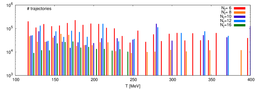
For the present analysis we use five lattice spacings for each temperature in the transition region, corresponding to the temporal resolutions and . We enriched our existing set of temperatures since Refs. Borsanyi:2010bp ; Borsanyi:2010cj and four-folded the statistics at . We save a configuration every tenth trajectory in a hybrid monte carlo stream with unit trajectory length. The statistics used in this analysis is given in Fig. 1, summed in bins of 10 MeV.
3.3 Fluctuations from the lattice
The fluctuations of interest are derivatives of the free energy with respect to the chemical potential of a conserved charge. This guarantees the finiteness of the lattice observables, thus no renormalization is necessary.
A derivative of the partition function can be written in terms of , the action with all fermionic degrees of freedom already integrated out, as follows:
| (10) |
When we take further derivatives, the following chain rule applies:
| (11) |
Here indicates the variable of the derivative, the chemical potential in this case, with or . and are the first and second derivatives of without the factor . Their ensemble averages are calculated with the same weight used for generating the configurations.
In our case and are
| (12) | |||||
| (13) |
with is the fermion operator with the bare mass , that we also used for generating these configurations. and stand for its first and second derivatives with respect to , respectively. The pre-factor is required by the staggered formulation of the single flavor trace. These derivatives are mass independent. In the lattice simulation as well as in the subsequent analysis, the bare mass is the only parameter that identifies a particular type of quark. The , and quantum numbers are provided by Eq. (1).
Ref. Gottlieb:1988cq describes a stochastic technique for calculating the traces in Eqs. (12) and (13). The traces are rewritten in terms of inner products of random sources. The most expensive part of the present analysis is the calculation of the trace in Eq. (12), which contains disconnected contributions and appears in almost all susceptibilities as . It required 128 pairs of random sources per configuration (256 for ). For each pair of sources one needs two inversions of the fermion matrix with the light quark mass.
3.4 Continuum extrapolation
With five lattice spacings per temperature we are in the position to go beyond the simplest form of continuum extrapolation and fit a second order polynomial in . Especially at low temperatures, such fit is indeed necessary, as the coarser lattices have corrections beyond the term. In general, a continuum fit benefits from higher order terms, but this also introduces ambiguities, such as whether it is appropriate to keep the coarsest point in the continuum extrapolation. The answer to this question is obtained by performing all possible extrapolations, and weighting them by the resulting goodness of the fit. Accordingly, we varied the number of included lattice spacings and made a linear and a quadratic fit in . We double the number of such choices by considering extrapolations of the inverse fluctuations () too, and then taking the inverse of the corresponding continuum result.
There is another source of systematic error: the interpolation ambiguity. The ensembles were not taken exactly at the same temperatures for different values, and the spline fit on the data for a given depends on the node points. We take two choices of the node points into the analyses (selecting the original temperature values with either even or odd indices). In most cases the two interpolations agree within statistical errors. We incorporated the systematic error from this source into the statistical error of the interpolating data points prior to the continuum fit. We selected the temperature range for each data set such that a consistent interpolation is possible.
This procedure has (with few exceptions) preferred the full quartic fit over four or five points in the transition region, and a suppressed quartic term fit for MeV. In most cases the reciprocal fit was preferred over the original variant.
We systematic errors are defined through the central 68.2% of the weighted distribution of all analyses, following our collaboration’s standard technique c.f. arXiv:0906.3599 ; Durr:2010aw . For simplicity, we give our results with the sum of the statistical and the symmetrized systematic errors. The continuum bands in the results section correspond to this combined error around a central value. In most cases the systematic error dominates. For and the two types of errors are of equal magnitude. The actual smallness of makes the relative combined error grow beyond 50%, thus we dropped this observable from our result list.
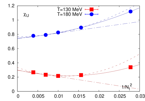
We give one example of our interpolation strategy in Fig. 2. We plot the measured values with statistical errors for two different temperatures. The data points seem to lie on a parabola, when plotted as a function of . We give three fits for each of the selected temperatures to indicate the spread of the possible continuum results.
As discussed in Ref. Borsanyi:2010cj one can use the tree level improvement program for observables. Independently whether one used it or not the results are the same (c.f. Figure 8 of Ref. Borsanyi:2010cj ). For simplicity we use in the present paper the direct method and do not apply the tree level improvement for our observables when we extrapolate to the continuum limit. The improvement factors for the various discretizations (, , , , ) are merely used here for plotting the raw lattice data.
4 Results
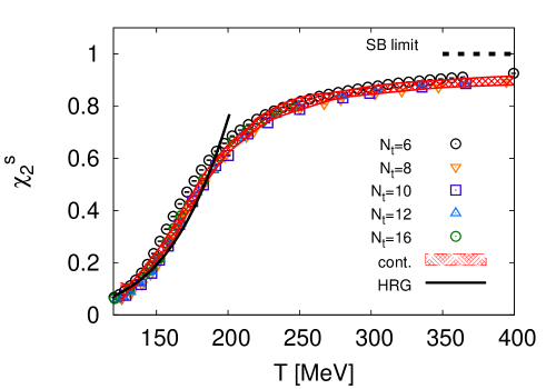
The first observables we discuss are the diagonal light and strange quark number susceptibilities: their behavior as functions of the temperature is shown in the two panels of Fig. 3. The different symbols correspond to different values of , from 8 to 16. The red band is the continuum extrapolation, obtained from the unimproved data, not from the improved ones. The continuum extrapolation is performed through a parabolic fit in the variable , over five values from 6 to 16. The band shows the spread of the results of other possible fits, as discussed in Section 3.4. The comparison between the improved data and the continuum bands in the figure shows the success of the improvement program throughout the entire temperature range. But even the unimproved data could be easily fitted for a continuum limit, the combined errors are below 3% in the deconfined phase. Both observables show a rapid rise in a certain temperature range, and reach approximately 90% of the ideal gas value at large temperatures. However, the temperature around which the susceptibilities rise is approximately 15-20 MeV larger for strange quarks than for light quarks. In addition, the light quark susceptibility shows a steeper rise with temperature, compared to the strange quark one. As expected, they approach each other at high temperatures. The effect more evident in Figure 4: in the left panel we show the continuum extrapolation of both susceptibilities on the same plot. In the right panel we show the ratio : it reaches 1 only around 300 MeV, while for smaller temperatures it is . It is worth noticing that all these observables agree with the corresponding HRG model predictions for temperatures below the transition.
The pattern of temperature dependence is strongly related the actual quark mass. The difference between the light and strange susceptibilities here with physical masses is more pronounced than in earlier works with not so light pions (see E.g. Ref. hotQCD2 ).


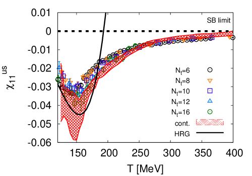
The non-diagonal susceptibility measures the degree of correlation between different flavors. This observable vanishes in the limit of an ideal, non-interacting QGP. However, Hard Thermal and Dense Loop framework provides a non-vanishing value for this correlation also at large temperatures Blaizot:2001vr . We show our result in Fig. 5. is non-zero in the entire temperature range under study. It has a dip in the crossover region, where the correlation between and quarks turns out to be maximal. It agrees with the HRG model prediction in the hadronic phase. This correlation stays finite and large for a certain temperature range above . A quantitative comparison between lattice results and predictions for a purely partonic QGP state can give us information about bound states survival above Ratti:2011au .
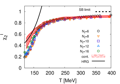
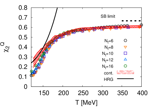
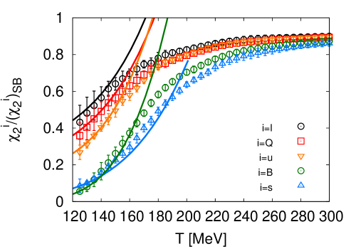
Quadratic baryon number, electric charge and isospin fluctuations can be obtained from the above partonic susceptibilities through Eqs. (7). We show our results for these observables in Fig. 6 and in the left panel of Fig. 7. In the low-temperature, hadronic phase we have a very good agreement with the HRG model predictions. In the crossover region these quantities all show a rapid rise with temperature, in analogy with what already observed for the light and strange quark susceptibilities. At large temperature they reach approximately 90% of their respective ideal gas values. A comparison between all diagonal susceptibilities, rescaled by their corresponding Stefan-Boltzmann limits, is shown in the right panel of Fig. 7, from which it is evident that they all show similar features in their temperature dependence, even if the temperature at which they rise is larger for the strangeness and baryon number susceptibilities.

The baryon-strangeness correlator defined in Eq. (8) was proposed long ago Koch:2005vg as a diagnostic for strongly interacting matter. It is supposed to be equal to one for a non-interacting QGP, while it is temperature-dependent and generally smaller than one in a hadronic system. We show our result for this observable in Fig. 8. At the smallest temperatures it agrees with the HRG model result, and it shows a rapid rise across the transition. It reaches the ideal gas limit much faster than the other observables under study, yet there is a window of about 100 MeV above , where its value is still smaller than one. In analogy with , this observable also gives us information on bound state survival above .

For convenience we tabulate our continuum results in Table 1.
5 Conclusions
In this paper we have presented the continuum results of our collaboration on diagonal and non-diagonal quark number susceptibilities, in a system with 2+1 staggered dynamical quark flavors with physical masses, in a temperature range between 125 and 400 MeV. The continuum extrapolations were based on and lattices. We calculated the systematic errors by varying over the ambiguities of the possible extrapolations.
All observables consistently show a very good agreement with the HRG model predictions for temperatures below the transition.
The diagonal fluctuations have some common features: they all show a rapid rise in the crossover region, and reach approximately 90% of the corresponding ideal gas value at large temperatures. The rise of both strange quark and baryon number susceptibilities is shifted to temperatures about 20 MeV higher than those for light quark, charge and isospin susceptibilities. Non-diagonal flavor and charge correlators remain different from their ideal gas values for a certain window of temperatures above the transition. This pattern encourages further studies to explore the possibility of bound state survival above .
| [MeV] | |||||||
|---|---|---|---|---|---|---|---|
| 125 | 0.432(92) | 0.268(39) | 0.239(45) | 0.085(37) | 0.019(2) | -0.0331(157) | 0.2492(811) |
| 130 | 0.481(87) | 0.311(19) | 0.269(44) | 0.101(10) | 0.027(8) | -0.0376(80) | 0.3442(492) |
| 135 | 0.523(78) | 0.359(15) | 0.300(42) | 0.124(15) | 0.040(12) | -0.0397(87) | 0.4426(573) |
| 140 | 0.566(59) | 0.405(22) | 0.327(34) | 0.155(16) | 0.055(15) | -0.0438(112) | 0.5040(355) |
| 145 | 0.614(40) | 0.448(30) | 0.358(27) | 0.190(19) | 0.070(13) | -0.0457(127) | 0.5672(484) |
| 150 | 0.641(34) | 0.496(36) | 0.376(17) | 0.226(16) | 0.087(11) | -0.0469(118) | 0.6416(442) |
| 155 | 0.669(41) | 0.548(24) | 0.400(22) | 0.261(20) | 0.106(12) | -0.0447(77) | 0.7090(278) |
| 160 | 0.696(25) | 0.580(29) | 0.420(20) | 0.295(28) | 0.124(8) | -0.0407(74) | 0.7575(152) |
| 165 | 0.722(28) | 0.618(21) | 0.440(18) | 0.346(26) | 0.143(7) | -0.0357(42) | 0.8024(160) |
| 170 | 0.747(20) | 0.659(15) | 0.460(14) | 0.400(21) | 0.160(5) | -0.0320(28) | 0.8398(163) |
| 175 | 0.753(28) | 0.699(17) | 0.480(19) | 0.441(23) | 0.179(6) | -0.0293(27) | 0.8697(133) |
| 180 | 0.780(31) | 0.733(17) | 0.499(18) | 0.491(23) | 0.194(6) | -0.0277(28) | 0.8931(89) |
| 185 | 0.799(24) | 0.760(16) | 0.502(15) | 0.533(21) | 0.207(6) | -0.0241(14) | 0.9132(59) |
| 190 | 0.810(17) | 0.770(13) | 0.513(10) | 0.568(18) | 0.218(5) | -0.0227(21) | 0.9317(38) |
| 200 | 0.827(15) | 0.799(15) | 0.530(10) | 0.636(15) | 0.235(5) | -0.0197(22) | 0.9457(35) |
| 220 | 0.860(13) | 0.844(14) | 0.561(9) | 0.732(20) | 0.259(4) | -0.0151(17) | 0.9616(52) |
| 240 | 0.881(18) | 0.868(16) | 0.578(12) | 0.791(22) | 0.273(6) | -0.0107(11) | 0.9741(46) |
| 260 | 0.890(16) | 0.880(15) | 0.586(11) | 0.823(20) | 0.282(5) | -0.0073(10) | 0.9822(54) |
| 280 | 0.895(12) | 0.888(12) | 0.592(8) | 0.845(12) | 0.287(4) | -0.0052(7) | 0.9866(30) |
| 300 | 0.900(14) | 0.895(15) | 0.596(9) | 0.861(15) | 0.291(5) | -0.0040(6) | 0.9889(27) |
| 320 | 0.904(15) | 0.900(16) | 0.600(10) | 0.873(15) | 0.294(5) | -0.0033(8) | 0.9905(22) |
| 340 | 0.908(14) | 0.905(15) | 0.603(9) | 0.882(14) | 0.297(5) | -0.0028(11) | 0.9920(20) |
| 360 | 0.911(14) | 0.908(14) | 0.605(9) | 0.889(14) | 0.299(5) | -0.0024(9) | 0.9932(34) |
| 380 | 0.913(15) | 0.911(15) | 0.607(10) | 0.894(16) | 0.300(5) | -0.0018(10) | 0.9943(39) |
| 400 | 0.915(16) | 0.913(17) | 0.608(11) | 0.899(16) | 0.302(5) | -0.0012(11) | 0.9953(36) |
Acknowledgments
Computations were carried out at the Universities Wuppertal, Budapest and Forschungszentrum Juelich. This work is supported in part by the Deutsche Forschungsgemeinschaft grants FO 502/2 and SFB- TR 55 and by the EU (FP7/2007-2013)/ERC no. 208740, as well as the Italian Ministry of Education, Universities and Research under the Firb Research Grant RBFR0814TT. We acknowledge the fruitful discussions with Alexei Bazavov, Christian Hölbling, Volker Koch and Krzysztof Redlich.
References
- (1) Y. Aoki, G. Endrodi, Z. Fodor, S. D. Katz and K. K. Szabo, Nature 443 (2006) 675 [hep-lat/0611014].
- (2) A. Bazavov, T. Bhattacharya, M. Cheng, C. DeTar, H. T. Ding, S. Gottlieb, R. Gupta and P. Hegde et al., arXiv:1111.1710 [hep-lat].
- (3) S. Jeon and V. Koch, Phys. Rev. Lett. 85, 2076 (2000)
- (4) M. Asakawa, U. W. Heinz and B. Muller, Phys. Rev. Lett. 85, 2072 (2000)
- (5) S. A. Gottlieb, W. Liu, D. Toussaint, R. L. Renken, R. L. Sugar, Phys. Rev. Lett. 59, 2247 (1987). Phys. Rev. D38, 2888-2896 (1988).
- (6) R. V. Gavai, J. Potvin, S. Sanielevici, Phys. Rev. D40, 2743 (1989).
- (7) L. D. McLerran, Phys. Rev. D36, 3291 (1987).
- (8) R. Dashen, S. K. Ma and H. J. Bernstein, Phys. Rev. 187, 345 (1969). R. Venugopalan and M. Prakash, Nucl. Phys. A 546, 718 (1992). F. Karsch, K. Redlich and A. Tawfik, Eur. Phys. J. C 29, 549 (2003) [arXiv:hep-ph/0303108]. F. Karsch, K. Redlich and A. Tawfik, Phys. Lett. B 571, 67 (2003) [arXiv:hep-ph/0306208]. A. Tawfik, Phys. Rev. D 71, 054502 (2005) [arXiv:hep-ph/0412336].
- (9) J. P. Blaizot, E. Iancu, A. Rebhan, Phys. Lett. B523, 143-150 (2001). [hep-ph/0110369].
- (10) C. Ratti, R. Bellwied, M. Cristoforetti, M. Barbaro, [arXiv:1109.6243 [hep-ph]].
- (11) V. Koch, A. Majumder and J. Randrup, Phys. Rev. Lett. 95, 182301 (2005)
- (12) R. V. Gavai, S. Gupta, P. Majumdar, Phys. Rev. D65, 054506 (2002). [hep-lat/0110032]. C. R. Allton, et. al. Phys. Rev. D66, 074507 (2002). [hep-lat/0204010]. C. R. Allton, et. al. Phys. Rev. D68, 014507 (2003). [arXiv:hep-lat/0305007 [hep-lat]]. C. R. Allton, et. al. Phys. Rev. D71, 054508 (2005). [hep-lat/0501030]. R. V. Gavai, S. Gupta, Phys. Rev. D72, 054006 (2005). [hep-lat/0507023]. S. Ejiri, F. Karsch, K. Redlich, Phys. Lett. B633, 275-282 (2006). [hep-ph/0509051].
- (13) R. V. Gavai, S. Gupta, Phys. Rev. D73, 014004 (2006). [hep-lat/0510044]. M. Cheng,, et. al. Phys. Rev. D79, 074505 (2009). [arXiv:0811.1006 [hep-lat]]; A. Bazavov, et. al. Phys. Rev. D 80, 014504 (2009).
- (14) S. Borsanyi, Z. Fodor, C. Hoelbling, S. Katz, S. Krieg, C. Ratti, K. Szabo, JHEP 1009, 073 (2010)
- (15) Y. Aoki, Z. Fodor, S. D. Katz and K. K. Szabo, Phys. Lett. B 643, 46 (2006)
- (16) Y. Aoki, S. Borsanyi, S. Durr, Z. Fodor, S. Katz, S. Krieg and K. Szabo, JHEP 0906, 088 (2009)
- (17) Y. Aoki, Z. Fodor, S. D. Katz and K. K. Szabo, JHEP 0601, 089 (2006)
- (18) C. Morningstar and M. J. Peardon, Phys. Rev. D 69, 054501 (2004)
- (19) E. Follana et al. [HPQCD and UKQCD Collaborations], Phys. Rev. D 75 (2007) 054502 [hep-lat/0610092].
- (20) Z. Fodor and S. D. Katz, arXiv:0908.3341 [hep-ph].
- (21) S. Borsanyi, G. Endrodi, Z. Fodor, A. Jakovac, S. D. Katz, S. Krieg, C. Ratti, K. K. Szabo, JHEP 1011, 077 (2010). [arXiv:1007.2580 [hep-lat]].
- (22) S. Durr, Z. Fodor, J. Frison, C. Hoelbling, R. Hoffmann, S. D. Katz, S. Krieg and T. Kurth et al., Science 322 (2008) 1224 [arXiv:0906.3599 [hep-lat]].
- (23) S. Durr, Z. Fodor, C. Hoelbling, S. D. Katz, S. Krieg, T. Kurth, L. Lellouch and T. Lippert et al., JHEP 1108 (2011) 148 [arXiv:1011.2711 [hep-lat]].