LPN11-94

IFIC/11-72

ZU-TH 27/11

Space-like (vs. time-like) collinear limits in QCD:
is factorization violated?

Stefano Catani ^(a), Daniel de Florian ^(b)(c) and Germán Rodrigo ^(d)

^(a)INFN, Sezione di Firenze and Dipartimento di Fisica e Astronomia,

Università di Firenze, I-50019 Sesto Fiorentino, Florence, Italy

^(b)Departamento de Física and IFIBA, FCEYN, Universidad de Buenos Aires,

(1428) Pabellón 1 Ciudad Universitaria, Capital Federal, Argentina

^(c)Institut für Theoretische Physik, Universität Zürich, CH-8057 Zürich, Switzerland

^(d)Instituto de Física Corpuscular, UVEG - Consejo Superior de Investigaciones Científicas, Parc Cientìfic, E-46980 Paterna (Valencia), Spain

Abstract

We consider the singular behaviour of QCD scattering amplitudes in kinematical configurations where two or more momenta of the external partons become collinear. At the tree level, this behaviour is known to be controlled by factorization formulae in which the singular collinear factor is universal (process independent). We show that this strict (process-independent) factorization is not valid at one-loop and higher-loop orders in the case of the collinear limit in space-like regions (e.g., collinear radiation from initial-state partons). We introduce a generalized version of all-order collinear factorization, in which the space-like singular factors retain some dependence on the momentum and colour charge of the non-collinear partons. We present explicit results on one-loop and two-loop amplitudes for both the two-parton and multiparton collinear limits. At the level of squared amplitudes and, more generally, cross sections in hadron–hadron collisions, the violation of strict collinear factorization has implications on the non-abelian structure of logarithmically-enhanced terms in perturbative calculations (starting from the next-to-next-to-leading order) and on various factorization issues of mass singularities (starting from the next-to-next-to-next-to-leading order).

LPN11-94

December 2011

1 Introduction

A relevant topic in QCD and, more generally, gauge field theories is the structure of the perturbative scattering amplitudes in various infrared (soft and collinear) regions. Virtual partonic fluctuations (i.e. partons circulating in loops) in the infrared (IR) region lead to divergent contributions to scattering amplitudes in four space-time dimensions. Real radiation of soft and collinear partons produces kinematical singularities, which also lead to IR divergent contributions after integration over the phase space of the emitted partons.

In the context of dimensional regularization, the (virtual) IR divergences of QCD amplitudes have been studied [1, 2, 3, 4, 5, 6, 7, 8] at one-loop, two-loop and higher-loop orders. The singularity structure related to (single and multiple) soft-parton radiation has been explicitly worked out [9, 10, 11, 12, 13, 14] in the cases of tree-level, one-loop and two-loop scattering amplitudes.

These studies and the ensuing understanding of (virtual) IR divergences and (real) soft-parton singularities rely on general factorization properties of QCD. The structure of the IR divergences and of the soft-parton singularities is described by corresponding factorization formulae. The divergent or singular behaviour is captured by factors that have a high degree of universality or, equivalently, a minimal process dependence (i.e. a minimal dependence on the specific scattering amplitude). To be precise, the divergent or singular factors depend on the momenta and quantum numbers (flavour, colour) of the external QCD partons in the scattering amplitude, while the detailed internal structure of the scattering amplitude plays no active role. Of course, in the case of soft-parton radiation, the singular factors also depend on the momenta and quantum numbers of the emitted soft partons.

In this paper we deal with collinear-parton singularities. The singular behaviour of QCD amplitudes, in kinematical configurations where two or more external-parton momenta become collinear, is also described by factorization formulae.

Considering the case of two collinear partons at the tree level, the collinear-factorization formula for QCD squared amplitudes was derived in a celebrated paper [15]. The corresponding factorization for QCD amplitudes (rather than squared amplitudes) was introduced in Refs. [16, 17]. At the tree level, the multiple collinear limit of three, four or more partons has been studied [18, 19, 11, 20, 21, 22] for both amplitudes and squared amplitudes. In the case of one-loop QCD amplitudes, collinear factorization was introduced in Refs. [23, 24, 12, 25], by explicitly treating the collinear limit of two partons. Explicit, though partial, results for the triple collinear limit of one-loop amplitudes were presented in Ref. [26]. The two-parton collinear limit of two-loop amplitudes was explicitly computed in Refs. [27, 14]. The structure of collinear factorization of higher-loop amplitudes was discussed in Ref. [28].

The collinear-factorization formulae that we have just recalled are similar to the factorization formulae that apply to virtual IR divergences and soft-parton singularities. However, the collinear-factorization formulae are ‘more universal’. Indeed, the collinear singular factors only depend on the momenta and quantum numbers (flavour, colour, spin) of the collinear partons. In other words, the collinear singular factors have no dependence on the external non-collinear partons of the QCD amplitudes. Throughout this paper, this feature of collinear-parton factorization is denoted ‘strict’ collinear factorization.

Despite so many established results, in this paper we show that strict collinear factorization of QCD amplitudes is actually not valid beyond the tree level.

We are not going to show that some of the known results at one-loop, two-loop or higher-loop levels are not correct. We simply start from the observation that these results refer (either explicitly [26, 27, 14] or implicitly) to the collinear limit in a specific kinematical configuration. This is the configuration where all partons with collinear momenta are produced in the final state of the physical process that is described by the QCD amplitude. We refer to this configuration as the time-like (TL) collinear limit.

In the TL collinear limit, strict collinear factorization is valid. In all the other kinematical configurations, generically denoted as space-like (SL) collinear limits, we find that strict collinear factorization is not valid (modulo some exceptional cases) beyond the tree level. We also show that, in the SL collinear limits, QCD amplitudes fulfill generalized factorization formulae, in which the collinear singular factors retain some dependence on the momenta and quantum numbers of the external non-collinear partons of the scattering amplitude.

The violation of strict collinear factorization is due to long-range (gauge) loop interactions between the collinear and non-collinear partons. These virtual radiative corrections produce absorptive contributions that, due to causality, distinguish initial-state from final-state interactions. In the TL collinear region, all the collinear partons are produced in the final state and strict factorization is recovered because of QCD colour coherence (i.e., the coherent action of the system of collinear partons). The SL collinear region involves collinear partons in both the initial and final states and, therefore, causality limits the factorization power of colour coherence.

Owing to their absorptive (’imaginary’) origin, strict-factorization breaking effects partly cancel at the level of squared amplitudes and, hence, in order-by-order perturbative calculations of physical observables. Indeed, we find that such a cancellation is complete up to the next-to-leading order (NLO). Nonetheless, strict factorization is violated at higher orders. For instance, the simplest subprocess in which strict collinear factorization is definitely violated at the squared amplitude level is $2\rightarrow 3$ parton scattering, in the kinematical configurations where one of the three final-state partons is collinear or almost collinear to one of the two initial-state partons. In this subprocess we find non-abelian factorization breaking effects that first occur at the two-loop level. Therefore, these effects contribute to hard-scattering processes in hadron–hadron collisions: they produce next-to-next-to-leading order (NNLO) logarithmic contributions to three jet production with one low-$p_{T}$ jet (the low-$p_{T}$ jet is originated by the final-state parton that is almost collinear to one of initial-state partons), and next-to-next-to-next-to-leading order (N³LO) contributions to one-jet and di-jet inclusive production.

The strict factorization breaking effects uncovered in the simple example of $2\rightarrow 3$ parton scattering have more general implications in the context of perturbative QCD computations of jet and hadron production in hadron–hadron collisions. Starting from the N³LO in perturbation theory, these effects severely complicate the mechanism of cancellation of IR divergences that leads to the factorization theorem of mass (collinear) singularities [29]. These complications challenge the universal (process-independent) validity of mass-singularity factorization, and they are related to issues that arise in the context of factorization of transverse-momentum dependent distributions [30, 31, 32]. The perturbative resummation of large logarithmic terms produced by collinear parton evolution is also affected by the violation of strict collinear factorization: parton evolution gets tangled with the colour and kinematical structure of the hard-scattering subprocess, and this leads to the appearance of ‘entangled logarithms’. An example of entangled logarithms is represented by the class of ‘super-leading’ non-global logarithms discovered [33] in the N⁴LO computation of the dijet cross section with a large rapidity gap between the two jets. Indeed, the physical mechanism that produces those super-leading logarithms [34] is directly related to the mechanism that generates the violation of strict collinear factorization.

The outline of the paper is as follows. Sections 2–4 are devoted to the two-parton collinear limit. In Sect. 2, we consider tree-level amplitudes; we introduce our notation and, in particular, the colour space formulation based on the collinear splitting matrix. In Sect. 3, we review the known results on the TL collinear limit of one-loop amplitudes. The SL collinear limit at one-loop level is considered in Sect. 4. Here, we illustrate the violation of strict factorization, we introduce our generalized form of collinear factorization, and we present the result of the one-loop splitting matrix to all-orders in the dimensional regularization parameter $\epsilon$. In Sect. 5, the study of the collinear behaviour of QCD amplitudes is extended to the multiparton collinear limit and beyond the one-loop level. In particular, we illustrate the violation of strict collinear factorization by deriving the explicit expression of the IR divergences (i.e., the $\epsilon$ poles) of the one-loop multiparton splitting matrix. In Sect. 6, we consider the all-order IR structure of the collinear splitting matrix, we present the explicit IR divergent terms at the two-loop level, and we discuss the ensuing new features of strict collinear factorization. In Sect. 7, we use our results on the collinear splitting matrix to compute the singular collinear behaviour of squared amplitudes. We explicitly show that strict collinear factorization is violated also at the squared amplitude level, and we comment on the implications for QCD calculations of hard-scattering cross sections in hadron–hadron collisions. In Sect. 8, we briefly summarize the main results. Additional technical details are presented in the Appendices. In Appendix A, we illustrate the violation of strict collinear factorization within the (colour-stripped) formulation in terms of colour subamplitudes and splitting amplitudes. In Appendix B, we explicitly compute the IR divergences of the two-loop splitting matrix. In Appendix C, we discuss how strict collinear factorization is recovered in the TL collinear region.

2 Collinear limit and tree-level amplitudes

We consider a generic scattering process that involves external QCD partons (gluons and massless quarks and antiquarks) and, possibly, additional non-QCD particles (e.g. partons with no colour such as leptons, photons, electroweak vector bosons, Higgs bosons and so forth). The corresponding $S$-matrix element (i.e., the on-shell scattering amplitude) is denoted by ${\cal M}(p_{1},p_{2},\dots,p_{n})$, where $p_{i}$ $(i=1,\dots,n)$ is the momentum of the QCD parton $A_{i}$ ($A_{i}=g,q$ or ${\bar{q}}$ ), while the dependence on the momenta of additional colourless particles is always understood.

The external QCD partons are on-shell $(p_{i}^{2}=0)$ and with physical spin polarizations (thus, ${\cal M}$ includes the corresponding spin wave functions). Note, however, that we always define the external momenta $p_{i}$’s as outgoing momenta. In particular, the time-component (i.e. the ‘energy’) $p_{i}^{0}$ of the momentum vector $p_{i}^{\mu}$ ($\mu=0,1,\dots,d-1$) in $d$ space-time dimensions is not positive definite. Different types of physical processes with $n$ external partons are described by applying crossing symmetry to the same matrix element ${\cal M}(p_{1},p_{2},\dots,p_{n})$. According to our definition of the momenta, if $p_{i}$ has positive energy, ${\cal M}(p_{1},p_{2},\dots,p_{n})$ describes a physical process that produces the parton $A_{i}$ in the final state; if $p_{i}$ has negative energy, ${\cal M}(p_{1},p_{2},\dots,p_{n})$ describes a physical process produced by the collision of the antiparton ${\overline{A}}_{i}$ in the initial state.

The matrix element ${\cal M}(p_{1},p_{2},\dots)$ can be evaluated in QCD perturbation theory as a power series expansion (i.e., loop expansion) in the QCD coupling $g_{\mathrm{S}}$ (or, equivalently, in the strong coupling $\alpha_{\mathrm{S}}=g_{\mathrm{S}}^{2}/(4\pi)$). We write

$${\cal M}={\cal M}^{(0)}+{\cal M}^{(1)}+{\cal M}^{(2)}+\dots\;\;,$$ (1)

where ${\cal M}^{(0)}$ is the tree-level scattering amplitude, ${\cal M}^{(1)}$ is the one-loop scattering amplitude, ${\cal M}^{(2)}$ is the two-loop scattering amplitude, and so forth. Note that in Eq. (1) we have not written down any power of $g_{\mathrm{S}}$. Thus, ${\cal M}^{(0)}$ includes an integer power of $g_{\mathrm{S}}$ as overall factor, and ${\cal M}^{(1)}$ includes an extra factor of $g_{\mathrm{S}}^{2}$ (i.e., ${\cal M}^{(1)}/{\cal M}^{(0)}\propto g_{\mathrm{S}}^{2}$). Throughout the first part of the paper (Sects. 2–5.2), we always consider unrenormalized matrix elements, and $g_{\mathrm{S}}$ denotes the bare (unrenormalized) coupling constant.

Physical processes take place in four-dimensional space time. In the four-dimensional evaluation of the one-loop amplitude ${\cal M}^{(1)}$ one encounters ultraviolet and IR divergences that have to be properly regularized. The most efficient method to simultaneously regularize both kind of divergences in gauge theories is dimensional regularization in $d\neq 4$ space-time dimensions. We work in $d=4-2\epsilon$ space-time dimensions, and the dimensional-regularization scale is denoted by $\mu$. Unless otherwise stated, throughout the paper we formally consider expressions for arbitrary values of $d=4-2\epsilon$ (equivalently, in terms of $\epsilon$-expansions, the expressions are valid to all orders in $\epsilon$).

We are interested in studying the behaviour of ${\cal M}(p_{1},p_{2},\dots,p_{n})$ in the kinematical configuration where two of the external parton momenta become (almost) collinear. Without loss of generality, we assume that these momenta are $p_{1}$ and $p_{2}$. We parametrize these momenta as follows:

$$p_{i}^{\mu}=x_{i}\,p^{\mu}+k_{\perp i}^{\mu}-\frac{k_{\perp i}^{2}}{x_{i}}\frac{n^{\mu}}{2p\cdot n}\;,\quad\quad i=1,2\;,$$ (2)

where the light-like ($p^{2}=0$) vector $p^{\mu}$ denotes the collinear direction, while $n^{\mu}$ is an auxiliary light-like ($n^{2}=0$) vector, which is necessary to specify the transverse components $k_{\perp i}$ ($k_{\perp i}\cdot p=k_{\perp i}\cdot n=0$, with $k_{\perp i}^{2}<0$) or, equivalently, to specify how the collinear direction is approached. No other constraints are imposed on the longitudinal and transverse variables $x_{i}$ and $k_{\perp i}$ (in particular, we have $x_{1}+x_{2}\neq 1$ and $k_{\perp 1}+k_{\perp 2}\neq 0$). Thus, we can consider any (asymmetric) collinear limits at once. Note, however, that the collinear limit is invariant under longitudinal boosts along the direction of the total momentum $p_{12}^{\mu}=p_{1}^{\mu}+p_{2}^{\mu}$. Thus, the relevant (independent) kinematical variables are the following boost-invariant quantities: a single transverse-momentum variable ${\widetilde{k}}^{\mu}$ (${\widetilde{k}}^{\mu}=z_{2}k_{\perp 1}^{\mu}-z_{1}k_{\perp 2}^{\mu}$, ${\widetilde{k}}^{2}<0$) and a single longitudinal-momentum fraction, which can be either $z_{1}$ or $z_{2}$ (or the ratio between $z_{1}$ and $z_{2}$). The longitudinal-momentum fractions $z_{1}$ and $z_{2}$ are

$$z_{i}=\frac{x_{i}}{x_{1}+x_{2}}\;\;,\quad\quad z_{1}+z_{2}=1\;\;.$$ (3)

In terms of these boost-invariant variables, the invariant mass squared $s_{12}=(p_{1}+p_{2})^{2}$ of the system of the two ‘collinear’ partons is written as

$$s_{12}=2p_{1}\cdot p_{2}=-\frac{{\widetilde{k}}^{2}}{z_{1}\,z_{2}}\;\;.$$ (4)

We also define the following light-like $({\widetilde{P}}^{2}=0)$ momentum ${\widetilde{P}}^{\mu}$:

$${\widetilde{P}}^{\mu}=(p_{1}+p_{2})^{\mu}-\frac{s_{12}\;n^{\mu}}{2(p_{1}+p_{2})\cdot n}\;\;.$$ (5)

In the kinematical configuration where the parton momenta $p_{1}$ and $p_{2}$ become collinear, their invariant mass $s_{12}$ vanishes, and the matrix element ${\cal M}(p_{1},p_{2},\dots,p_{n})$ becomes singular. To precisely define the collinear limit, we rescale the transverse momenta $k_{\perp i}$ in Eq. (2) by an overall factor $\lambda$ (namely, $k_{\perp i}\rightarrow\lambda\;k_{\perp i}$ with $i=1,2$), and then we perform the limit $\lambda\rightarrow 0$. In this limit, the behaviour of the matrix element ${\cal M}(p_{1},p_{2},\dots,p_{n})$ is proportional to $1/\lambda$. We are interested in explicitly evaluating the matrix element contribution that controls this singular behaviour order by order in the perturbative expansion. More precisely, in $d=4-2\epsilon$ dimensions, the four-dimensional scaling behaviour in the collinear limit is modified by powers of $(\lambda^{2})^{-\epsilon}$. Since we work with fixed $\epsilon$, we treat the powers of $(\lambda^{2})^{-\epsilon}$ as contributions of order unity in the collinear limit.

In summary, considering the limit $s_{12}\rightarrow 0$, we are interested in the singular behaviour:

$${\cal M}(p_{1},p_{2},\dots,p_{n})\sim\frac{1}{\sqrt{s_{12}}}\;{\rm mod}\,(\ln^{k}s_{12})\;\Bigl{[}\,1+{\cal O}({\sqrt{s_{12}}}\;)\,\Bigr{]}\;\;,$$ (6)

where the logarithmic contributions $\ln^{k}s_{12}$ ($k=0,1,2,\dots)$ ultimately arise from the power series expansion in $\epsilon$ of terms such as $(s_{12})^{-\epsilon}$. These logarithmic contributions are taken into account in our calculation, while the corrections of relative order ${\cal O}({\sqrt{s_{12}}}\;)$ are systematically neglected.

As is well known [16, 17], the singular behaviour of tree-level scattering amplitudes in the collinear limit is universal (process independent) and factorized. The factorization structure is usually presented at the level of colour subamplitudes [17], in a colour-stripped form. In Ref. [26], we proposed a formulation of collinear factorization that is valid directly in colour space. Here, we follow this colour space formulation, which turns out to be particularly suitable to the main purpose of the present paper, namely, the general study of the SL collinear limit at one-loop and higher-loop orders.

To directly work in colour space, we use the notation of Ref. [35] (see also Ref. [1]). The scattering amplitude ${\cal M}$ depends on the colour indices $\{c_{1},c_{2},\dots\}$ and on the spin (e.g. helicity) indices $\{s_{1},s_{2},\dots\}$ of the external QCD partons; we write

$${\cal M}^{c_{1},c_{2},\dots,c_{n};s_{1},s_{2},\dots,s_{n}}(p_{1},p_{2},\dots,p_{n})\;\;.$$ (7)

We formally treat the colour and spin structures by introducing an orthonormal basis $\{|{c_{1},c_{2},\dots,c_{n}}\rangle\otimes|{s_{1},s_{2},\dots,s_{n}}\rangle\}$ in colour + spin space. The scattering amplitude in Eq. (7) can be written as

$${\cal M}^{c_{1},c_{2},\dots;s_{1},s_{2},\dots}(p_{1},p_{2},\dots)\equiv\Bigl{(}\langle{c_{1},c_{2},\dots}|\otimes\langle{s_{1},s_{2},\dots}|\Bigr{)}\;|{{\cal M}(p_{1},p_{2},\dots)}\rangle\;\;.$$ (8)

Thus $|{{\cal M}(p_{1},p_{2},\dots,p_{n})}\rangle$ is a vector in colour + spin (helicity) space.

As stated at the beginning of this section, we define the external momenta $p_{i}$’s as outgoing momenta. The colour indices $\{c_{1},c_{2},\dots\,c_{n}\}$ are consistently treated as outgoing colour indices: $c_{i}$ is the colour index of the parton $A_{i}$ with outgoing momentum $p_{i}$ (if $p_{i}$ has negative energy, $c_{i}$ is the colour index of the physical parton ${\overline{A}}_{i}$ that collides in the initial state). An analogous comment applies to spin indices.

Having introduced our notation, we can write down the colour-space factorization formula [26] for the collinear limit of the tree-level amplitude ${\cal M}^{(0)}$. We have

$$|{{\cal M}^{(0)}(p_{1},p_{2},\dots,p_{n})}\rangle\simeq{{\mbox{\boldmath$Sp$}}}^{(0)}(p_{1},p_{2};{\widetilde{P}})\;\;|{{\cal M}^{(0)}({\widetilde{P}},\dots,p_{n})}\rangle\;\;,$$ (9)

which is valid in any number $d=4-2\epsilon$ of dimensions. The only approximation (which is denoted by the symbol ‘$\simeq$’) involved on the right-hand side amounts to neglecting terms that are less singular in the collinear limit (i.e. the contributions denoted by the term ${\cal O}({\sqrt{s_{12}}}\;)$ in Eq. (6)).

The tree-level factorization formula (9) relates the original matrix element (on the left-hand side) with $n$ partons to a corresponding matrix element (on the right-hand side) with $n-1$ partons. The latter is obtained from the former by replacing the two collinear partons $A_{1}$ and $A_{2}$ (with momentum $p_{1}$ and $p_{2}$, respectively) with a single parent parton $A$, whose momentum is ${\widetilde{P}}$ (see Eq. (5)) and whose flavour is determined by flavour conservation of the QCD interactions. More precisely, $A$ is a quark (an antiquark) if the two collinear partons are a quark (an antiquark) and a gluon, and $A$ is a gluon otherwise.

The process dependence of Eq. (9) is entirely embodied in the matrix elements on both sides. The tree-level factor ${{\mbox{\boldmath$Sp$}}}^{(0)}(p_{1},p_{2};{\widetilde{P}})$, which encodes the singular behaviour in the collinear limit, is universal (process independent) and it does not depend on the non-collinear partons with momenta $p_{3},\dots,p_{n}$. It depends on the momenta and quantum numbers (flavour, spin, colour) of the partons that are involved in the collinear splitting $A\rightarrow A_{1}A_{2}$. According to our notation, ${{\mbox{\boldmath$Sp$}}}^{(0)}(p_{1},p_{2};{\widetilde{P}})$ is a matrix in colour+spin space, named the splitting matrix [26].

The splitting matrix acts between the colour space of the $n-1$ partons of $|{{\cal M}^{(0)}({\widetilde{P}},..,p_{n})}\rangle$ and the colour space of the $n$ partons of the original amplitude $|{{\cal M}^{(0)}(p_{1},p_{2},..,p_{n})}\rangle$. Because ${{\mbox{\boldmath$Sp$}}}^{(0)}(p_{1},p_{2};{\widetilde{P}})$ does not depend on the non-collinear partons, their colour is left unchanged in Eq. (9) (precisely speaking, ${{\mbox{\boldmath$Sp$}}}^{(0)}$ is proportional to the unit matrix in the colour subspace of the non-collinear partons). The only non-trivial dependence on the colour (and spin) indices is due to the partons that undergo the collinear splitting $A\rightarrow A_{1}A_{2}$. Making this dependence explicit, we have

$$Sp^{(0)\;(c_{1},c_{2};\,c)}(p_{1},p_{2};{\widetilde{P}})\equiv\langle{c_{1},c_{2}}|\;{{\mbox{\boldmath$Sp$}}}^{(0)}(p_{1},p_{2};{\widetilde{P}})\;|{c}\rangle\;\;,$$ (10)

where $c_{1},c_{2}$ and $c$ are the colour indices of the partons $A_{1},A_{2}$ and the parent parton $A$. The colour indices of gluons, quarks and antiquarks are actually different; we use the notation $c=\{a\}=1,\dots,N_{c}^{2}-1$ for gluons and $c=\{\alpha\}=1,\dots,N_{c}$ for quarks and antiquarks, where $N_{c}$ is the number of colours. A colour matrix of the fundamental representation of the gauge group is denoted by $t^{a}_{\alpha_{1}\alpha_{2}}\,$, and the structure constants are $f_{abc}\,$; we use the following normalization:

$$[t^{a},t^{b}]=if_{abc}t^{c}\;\;,\quad{\rm Tr}\left(t^{a}t^{b}\right)=\frac{1}{2}\,\delta^{ab}\;\;.$$ (11)

The matrices $t^{a}$ are hermitian ($(t^{a})^{\dagger}=(t^{a})$) and the structure constants $f_{abc}$ are real ($f_{abc}^{*}=f_{abc}$). There are four different flavour-conserving configurations $A\rightarrow A_{1}A_{2}$. The corresponding explicit form of the tree-level splitting matrix is:

$q\rightarrow q_{1}g_{2}$

$$Sp_{q_{1}g_{2}}^{(0)\;(\alpha_{1},a_{2};\,\alpha)}(p_{1},p_{2};{\widetilde{P}})=\mu^{\epsilon}\,g_{\mathrm{S}}\;t^{a_{2}}_{\alpha_{1}\alpha}\;\frac{1}{s_{12}}\;{\overline{u}}(p_{1})\,{\ooalign{$\hfil/\hfil$\crcr${\varepsilon}$}}(p_{2})\,u({\widetilde{P}})\;\;,$$ (12)

${\bar{q}}\rightarrow{\bar{q}}_{1}g_{2}$

$$Sp_{{\bar{q}}_{1}g_{2}}^{(0)\;(\alpha_{1},a_{2};\,\alpha)}(p_{1},p_{2};{\widetilde{P}})=\mu^{\epsilon}\,g_{\mathrm{S}}\;\left(-t^{a_{2}}_{\alpha\,\alpha_{1}}\right)\;\frac{1}{s_{12}}\;{\overline{v}}({\widetilde{P}})\,{\ooalign{$\hfil/\hfil$\crcr${\varepsilon}$}}(p_{2})\,v(p_{1})\;\;,$$ (13)

$g\rightarrow q_{1}{\bar{q}}_{2}$

$$Sp_{q_{1}{\bar{q}}_{2}}^{(0)\;(\alpha_{1},\alpha_{2};\,a)}(p_{1},p_{2};{\widetilde{P}})=\mu^{\epsilon}\,g_{\mathrm{S}}\;t^{a}_{\alpha_{1}\alpha_{2}}\;\frac{1}{s_{12}}\;{\overline{u}}(p_{1})\,{\ooalign{$\hfil/\hfil$\crcr${\varepsilon}$}}^{*}({\widetilde{P}})\,v(p_{2})\;\;,$$ (14)

$g\rightarrow g_{1}g_{2}$

$$Sp_{g_{1}g_{2}}^{(0)\;(a_{1},a_{2};\,a)}(p_{1},p_{2};{\widetilde{P}}) \!\!\!\!\!\!\!\!\!=\mu^{\epsilon}\,g_{\mathrm{S}}\;i\;f_{a_{1}a_{2}\,a}\;\frac{2}{s_{12}}$$

$$\!\!\!\!\!\!\!\!\!\!\!\!\!\!\!\!\!\!\!\!\!\!\!\!\!\!\!\!\!\!\!\!\!\!\!\!\!\!\!\!\!\!\!\times\left[{\varepsilon}(p_{1})\cdot{\varepsilon}(p_{2})\;p_{1}\cdot{\varepsilon}^{*}({\widetilde{P}})+{\varepsilon}(p_{2})\cdot{\varepsilon}^{*}({\widetilde{P}})\;p_{2}\cdot{\varepsilon}(p_{1})-{\varepsilon}(p_{1})\cdot{\varepsilon}^{*}({\widetilde{P}})\;p_{1}\cdot{\varepsilon}(p_{2})\right]\;\;,$$

where $u(p)$ and $v(p)$ are the customary Dirac spinors and ${\varepsilon}^{\mu}(p)$ is the physical polarization vector of the gluon (${\varepsilon}_{\mu}^{*}$ is the complex conjugate of ${\varepsilon}_{\mu}$). Spin indices play no relevant active role in the context of the main discussion of the present paper. They are embodied in the parton wave functions $u,v,{\varepsilon}$ and are not explicitly denoted throughout the paper. The explicit expressions of Eqs. (12)–(2) in a definite helicity basis can be found in the literature (see, for instance, the Appendix A of the second paper in Ref. [12]).

We briefly comment on the relation between Eq. (9) and the customary collinear-factorization formulae for colour subamplitudes (see also the Appendix A). The colour-space factorization formula (9) is valid for a generic matrix element $|{{\cal M}^{(0)}(p_{1},p_{2},..,p_{n})}\rangle$; in particular, the factorization formula does not require any specifications about the colour structure of the matrix element. Collinear factorization of QCD scattering amplitudes is usually discussed [16] upon colour decomposition of the matrix element. The colour decomposition, whose actual form depends on the specific partonic content of the matrix element (e.g., on the number of gluons and quark-antiquark pairs), factorizes the QCD colour from colourless kinematical coefficients, which are called colour subamplitudes (see, e.g., Ref. [17]). Colour subamplitudes fulfil several process-independent properties, including collinear factorization. In the region where the two parton momenta $p_{1}$ and $p_{2}$ become collinear, the collinear-factorization formula of the colour subamplitudes is a colour-stripped analogue of Eq. (9): the colour vectors $|{{\cal M}^{(0)}}\rangle$ on both sides are replaced by corresponding colour subamplitudes, and the colour matrix ${{\mbox{\boldmath$Sp$}}}^{(0)}(p_{1},p_{2};{\widetilde{P}})$ is replaced by a universal kinematical function, which is called splitting amplitude and is usually denoted by ${\rm Split}^{(0)}(p_{1},p_{2};{\widetilde{P}})$ (see also the Appendix A).

In the case of the tree-level collinear splitting of two partons, the relation between the splitting matrix ${{\mbox{\boldmath$Sp$}}}^{(0)}$ and the splitting amplitude ${\rm Split}^{(0)}$ is particularly straightforward. Indeed, having fixed the flavour of the partons in the collinear splitting process $A\rightarrow A_{1}A_{2}$, the corresponding splitting matrix ${{\mbox{\boldmath$Sp$}}}^{(0)}$ involves a single (and unique) colour structure and, therefore, we have a direct proportionality relation:

$${{\mbox{\boldmath$Sp$}}}^{(0)}(p_{1},p_{2};{\widetilde{P}})\propto\left({\bf colour\;\;\;matrix}\right)\times{\rm Split}^{(0)}(p_{1},p_{2};{\widetilde{P}})\;\;,$$ (16)

where the colour matrix on the right-hand side is obtained by simple inspection of Eqs. (12)–(2) (see the colour factors $t^{a}_{\alpha\,\alpha^{\prime}}$ in Eqs. (12)–(14) and the colour factor $if_{a_{1}a_{2}a}$ in Eq. (2)).

As discussed at the beginning of this section, the outgoing momenta $p_{i}$’s of ${\cal M}(p_{1},\dots,p_{n})$, depending on the sign of their energy, actually describe different physical processes, which take place in different kinematical regions. Correspondingly, the collinear splitting $A\rightarrow A_{1}A_{2}$ formally describes different physical subprocesses, which take place in either the TL (if $p_{1}^{0}p_{2}^{0}>0$) or SL (if $p_{1}^{0}p_{2}^{0}<0$) regions. In these regions, the collinear variables $z_{1}$, $z_{2}$ and $s_{12}$ in Eqs. (3) and (4) are constrained as follows:

$${\rm TL}:\quad\quad\quad\quad\quad s_{12}>0\;\;,\quad z_{1}z_{2}>0\;\;,$$ (17)

$${\rm SL}:\quad\quad\quad\quad\quad s_{12}<0\;\;,\quad z_{1}z_{2}<0\;\;.$$ (18)

The most relevant physical subprocesses are the customary subprocesses:

• TL $\;\;\;(p_{1}^{0}>0\;,\;p_{2}^{0}>0$):

$$A^{*}\rightarrow A_{1}(z)\;A_{2}(1-z)\;\;,\quad{\rm with}\quad z=z_{1}=1-z_{2}\;,\;\;\;\;\,0<z<1\;\;,$$ (19)

• SL $\;\;\;(p_{1}^{0}<0\;,\;p_{2}^{0}>0\;,\;\widetilde{P}^{0}<0$):

$${\overline{A}}_{1}\rightarrow{\overline{A}}^{\;*}(z)\;A_{2}(1-z)\;\;,\quad{\rm with}\quad z=\frac{1}{z_{1}}=\frac{1}{1-z_{2}}\;,\;\;\;0<z<1\;\;.$$ (20)

In the TL subprocess of Eq. (19), the partons $A_{1}$, $A_{2}$ and the parent parton $A$ are physically produced into the final state; the collinear decay of the parent parton $A^{*}$, which is slightly off-shell (with positive virtuality) in the vicinity of the collinear limit, transfers the longitudinal-momentum fractions $z$ and $1-z$ to $A_{1}$ and $A_{2}$, respectively. In the SL subprocess of Eq. (20), the physical parton ${\overline{A}}_{1}$, which collides in the initial state, radiates the physical parton $A_{2}$, with longitudinal-momentum fraction $1-z$, in the final state; the remaining fraction, $z$, of longitudinal momentum is carried by the accompanying (‘parent’) parton ${\overline{A}}^{\;*}$ (which is slightly off-shell, with negative virtuality, in the vicinity of the collinear limit) that replaces ${\overline{A}}_{1}$ as physically colliding parton in the initial state.

There are two other physical subprocesses that are kinematically allowed: the TL subprocess ${\overline{A}}_{1}{\overline{A}}_{2}\rightarrow{\overline{A}}^{\;*}$ (parton–parton fusion into an initial-state parton) is allowed if $p_{1}^{0}$ and $p_{2}^{0}$ are both negative, and the SL subprocess ${\overline{A}}_{1}A^{*}\rightarrow A_{2}$ (parton–parton fusion into a final-state parton) is allowed if $p_{1}^{0}<0\;,\;p_{2}^{0}>0\;,$ and $\widetilde{P}^{0}>0$. The subprocess ${\overline{A}}_{1}{\overline{A}}_{2}\rightarrow{\overline{A}}^{\;*}$ (the initial-state parton ${\overline{A}}^{\;*}$ is produced by the fusion of the two initial-state collinear partons ${\overline{A}}_{1}$ and ${\overline{A}}_{2}$) occurs if ${\cal M}(p_{1},p_{2},\dots)$ corresponds to a physical process with at least three colliding particles in the initial state (the partons ${\overline{A}}_{1},{\overline{A}}_{2}$ and, at least, one additional particle). The subprocess ${\overline{A}}_{1}A^{*}\rightarrow A_{2}$ (the final-state parton $A_{2}$ is produced by the fusion of the initial-state parton ${\overline{A}}_{1}$ and the final-state parton $A^{*}$) occurs if ${\cal M}(p_{1},p_{2},\dots)$ corresponds to a physical process in which the initial state contains the parton ${\overline{A}}_{1}$ and, in addition, either one massive particle or (at least) two particles. Owing to these kinematical features, these subprocesses are less relevant in the context of QCD hard-scattering processes.

The splitting matrix ${{\mbox{\boldmath$Sp$}}}^{(0)}(p_{1},p_{2};{\widetilde{P}})$ in the factorization formula (9) applies to any physical subprocesses, in both the TL and SL regions. Strictly speaking, the explicit expressions in Eqs. (12)–(2) refer to the TL region where the energies of $p_{1},p_{2}$ and ${\widetilde{P}}$ are positive. The corresponding expressions in other kinematical regions are straightforwardly obtained by applying crossing symmetry. If the energy of the momentum $P$ ($P=p_{1},p_{2}$ or ${\widetilde{P}}$) is negative, the crossing relation simply amounts to the usual replacement of the corresponding wave function (i.e., $u(P)\leftrightarrow v(-P)$ and ${\varepsilon}(P)\leftrightarrow{\varepsilon}^{*}(-P)$).

3 One-loop amplitudes: time-like collinear limit

In this section we consider the collinear behaviour of the one-loop QCD amplitudes ${\cal M}^{(1)}$ in Eq. (1). We use the same general notation as in Sect. 2. However, we anticipate that the results are valid only in the case of the TL collinear splitting (i.e., $s_{12}>0$).

The singular behaviour of ${\cal M}^{(1)}(p_{1},p_{2},\dots,p_{n})$ in the region where the two momenta $p_{1}$ and $p_{2}$ become collinear is also described by a factorization formula. The extension of the tree-level colour-space formula (9) to one-loop amplitudes is [26]

$$|{{\cal M}^{(1)}(p_{1},p_{2},\dots,p_{n})}\rangle \simeq {{\mbox{\boldmath$Sp$}}}^{(1)}(p_{1},p_{2};{\widetilde{P}})\;\;|{{\cal M}^{(0)}(\widetilde{P},\dots,p_{n})}\rangle$$ (21)

$$+ {{\mbox{\boldmath$Sp$}}}^{(0)}(p_{1},p_{2};{\widetilde{P}})\;\;|{{\cal M}^{(1)}(\widetilde{P},\dots,p_{n})}\rangle\;\;.$$

The ‘reduced’ matrix elements on the right-hand side are obtained from ${\cal M}(p_{1},p_{2},\dots,p_{n})$ by replacing the two collinear partons $A_{1}$ and $A_{2}$ (with momentum $p_{1}$ and $p_{2}$, respectively) with their parent parton $A$, with momentum ${\widetilde{P}}$. The two contributions on the right-hand side are proportional to the reduced matrix element at the tree-level and at the one-loop order, respectively. The splitting matrix ${{\mbox{\boldmath$Sp$}}}^{(0)}$ is exactly the tree-level splitting matrix that enters Eq. (9). The one-loop splitting matrix ${{\mbox{\boldmath$Sp$}}}^{(1)}(p_{1},p_{2};{\widetilde{P}})$ encodes new (one-loop) information on the collinear splitting process $A\rightarrow A_{1}A_{2}$. Analogously to ${{\mbox{\boldmath$Sp$}}}^{(0)}$, the one-loop factor ${{\mbox{\boldmath$Sp$}}}^{(1)}(p_{1},p_{2};{\widetilde{P}})$ is a universal (process-independent) matrix in colour+spin space, and it only depends on the momenta and quantum numbers of the partons involved in the collinear splitting subprocess.

Within the colour subamplitude formulation, the collinear limit of two partons at the one-loop level was first discussed in Ref. [23] by introducing one-loop splitting amplitudes $\;{\rm Split}^{(1)}(p_{1},p_{2};{\widetilde{P}})$, which are the one-loop analogues of the tree-level splitting amplitudes mentioned in Sect. 2. A proof of collinear factorization of one-loop colour subamplitudes was presented in Ref. [24]. Explicit results for the splitting amplitudes $\,{\rm Split}^{(1)}\,$ in $d=4-2\epsilon$ dimensions (or, equivalently, the results to all orders in the $\epsilon$ expansion) were obtained in Refs. [12, 25].

The relation between the one-loop factorization formula (21) and its colour subamplitude version is exactly the same as the relation at the tree level (see also the Appendix A). The main point is that the one-loop splitting matrix ${{\mbox{\boldmath$Sp$}}}^{(1)}(p_{1},p_{2};{\widetilde{P}})$ involves a single colour structure (more precisely, there is a single colour structure for each flavour configuration of the splitting processes $A\rightarrow A_{1}A_{2}$), and this colour structure is the same structure that occurs in the tree-level splitting matrix ${{\mbox{\boldmath$Sp$}}}^{(0)}(p_{1},p_{2};{\widetilde{P}})$. In other words, the proportionality relation in Eq. (16) is valid also at the one-loop level: we can simply perform the replacements ${{\mbox{\boldmath$Sp$}}}^{(0)}(p_{1},p_{2};{\widetilde{P}})\rightarrow{{\mbox{\boldmath$Sp$}}}^{(1)}(p_{1},p_{2};{\widetilde{P}})$ and ${\rm Split}^{(0)}(p_{1},p_{2};{\widetilde{P}})\rightarrow{\rm Split}^{(1)}(p_{1},p_{2};{\widetilde{P}})$. Therefore, from the known $\,{\rm Split}^{(1)}\,$ [12, 25] we directly obtain the corresponding ${{\mbox{\boldmath$Sp$}}}^{(1)}$.

We now comment on the kinematical structure of ${{\mbox{\boldmath$Sp$}}}^{(1)}(p_{1},p_{2};{\widetilde{P}})$, i.e. on the momentum dependence of ${\rm Split}^{(1)}(p_{1},p_{2};{\widetilde{P}})$. Apart from the overall proportionality to the wave functions $u,v,{\varepsilon}$ of the collinear partons (which is analogous to that in Eqs. (12)–(2)), the kinematical structure [12, 25] depends on two different classes of contributions. One class contains all the contributions that have a rational dependence on the momenta; the other class contains transcendental functions (e.g., logarithms and polylogarithms) and, in particular, transcendental functions of the momentum fractions $z_{1}$ and $z_{2}$.

Considering $d=4-2\epsilon$ space-time dimensions, the one-loop integrals introduce the dimensional factor $\mu^{2\epsilon}$. Since the one-loop corrections to ${{\mbox{\boldmath$Sp$}}}^{(0)}(p_{1},p_{2};{\widetilde{P}})$ are dimensionless, ${{\mbox{\boldmath$Sp$}}}^{(1)}(p_{1},p_{2};{\widetilde{P}})$ necessarily includes the overall factor

$$\left(\frac{-s_{12}-i0}{\mu^{2}}\right)^{-\epsilon}\;\;,$$ (22)

where the $i0$ prescription follows from usual analyticity properties of the scattering amplitudes. Apart from this overall factor, the trascendental dependence of the two-parton collinear limit at one-loop order turns out to be entirely captured [12, 25] by a single hypergeometric function, namely, the function ${}_{2}F_{1}(1,-\epsilon;1-\epsilon;x)$. The integral representation of this hypergeometric function is

$${}_{2}F_{1}(1,-\epsilon;1-\epsilon;x)=-\,\epsilon\int_{0}^{1}\;dt\;t^{-1-\epsilon}\;(1-xt)^{-1}\;\;.$$ (23)

We thus define the following function:

$$f(\epsilon;1/x)\equiv\frac{1}{\epsilon}\;\Bigl{[}\;{}_{2}F_{1}(1,-\epsilon;1-\epsilon;1-x)-1\,\Bigr{]}\;\;.$$ (24)

The expansion of this function in powers of $\epsilon$ is as follows:

$$f(\epsilon;1/x)=\;\ln x-\epsilon\left[{\rm Li}_{2}(1-x)+\sum_{k=1}^{+\infty}\epsilon^{k}\;{\rm Li}_{k+2}(1-x)\right]\;,$$ (25)

where the dilogarithm function ${\rm Li}_{2}$ is

$${\rm Li}_{2}(x)\equiv-\int_{0}^{x}\;\frac{dt}{t}\;\ln(1-t)\;\;,$$ (26)

and the polylogarithms ${\rm Li}_{k+1}$ (with $k=2,3,\dots$) are defined [36] by

$${\rm Li}_{k+1}(x)\equiv\frac{\left(-1\right)^{k}}{(k-1)!}\;\int_{0}^{1}\;\frac{dt}{t}\;\left(\ln t\right)^{k-1}\;\ln(1-xt)\;\;.$$ (27)

As recalled in Sect. 2, there are four different flavour configurations in the collinear splitting process $A\rightarrow A_{1}A_{2}$. Considering the corresponding explicit results of Refs. [12, 25], the one-loop splitting matrix ${{\mbox{\boldmath$Sp$}}}^{(1)}(p_{1},p_{2};{\widetilde{P}})$ of Eq. (21) can be written in the following general (and compact) form:

$${{\mbox{\boldmath$Sp$}}}^{(1)}(p_{1},p_{2};{\widetilde{P}})={{\mbox{\boldmath$Sp$}}}^{(1)}_{H}(p_{1},p_{2};{\widetilde{P}})+I_{C}(p_{1},p_{2};{\widetilde{P}})\;{{\mbox{\boldmath$Sp$}}}^{(0)}(p_{1},p_{2};{\widetilde{P}})\;\;.$$ (28)

The factor $I_{C}(p_{1},p_{2};{\widetilde{P}})$ is specified below. Having specified this factor, the term ${{\mbox{\boldmath$Sp$}}}^{(1)}_{H}$ on the right-hand side of Eq. (28) can be extracted, in explicit form, from the results in Refs. [12, 25]. We do not report the explicit form of ${{\mbox{\boldmath$Sp$}}}^{(1)}_{H}$, since it has no relevant role in our discussion of the relation between the TL and SL collinear limits. In this respect, the only relevant property of ${{\mbox{\boldmath$Sp$}}}^{(1)}_{H}$ (which follows from our definition of $I_{C}$) is that it contains only terms with rational dependence on the momenta $p_{1},p_{2}$ and ${\widetilde{P}}$. Moreover, all the terms of ${{\mbox{\boldmath$Sp$}}}^{(1)}$ that are IR or ultraviolet divergent in $d=4$ dimensions (i.e. all the $\epsilon$ poles) are collected in the factor $I_{C}$ and, thus, removed from ${{\mbox{\boldmath$Sp$}}}^{(1)}_{H}$. Therefore, ${{\mbox{\boldmath$Sp$}}}^{(1)}_{H}$ is finite if we set $\epsilon=0$.

The term $I_{C}\times{{\mbox{\boldmath$Sp$}}}^{(0)}$ on the right-hand side of Eq. (28) contains all the IR and ultraviolet divergences of ${{\mbox{\boldmath$Sp$}}}^{(1)}$ and, more importantly, it collects the entire dependence of the collinear behaviour at one-loop order on transcendental functions (modulo the function in Eq. (22), which also appears in ${{\mbox{\boldmath$Sp$}}}^{(1)}_{H}$). The explicit expression of the factor $I_{C}$ for a generic splitting process $A\rightarrow A_{1}A_{2}$ is

$$I_{C}(p_{1},p_{2};{\widetilde{P}}) = \;g_{\mathrm{S}}^{2}\;c_{\Gamma}\;\left(\frac{-s_{12}-i0}{\mu^{2}}\right)^{-\epsilon}$$

$$\times \left\{\;\frac{1}{\epsilon^{2}}\;\Bigl{(}C_{12}-C_{1}-C_{2}\Bigr{)}+\frac{1}{\epsilon}\;\Bigl{(}\gamma_{12}-\gamma_{1}-\gamma_{2}+b_{0}\Bigr{)}\right.$$

$$- \left.\;\frac{1}{\epsilon}\,\left[\Bigl{(}C_{12}+C_{1}-C_{2}\Bigr{)}\;f(\epsilon;z_{1})+\Bigl{(}C_{12}+C_{2}-C_{1}\Bigr{)}\;f(\epsilon;z_{2})\;\right]\right\}\;\;,$$

where $c_{\Gamma}$ is the typical volume factor of $d$-dimensional one-loop integrals:

$$c_{\Gamma}\equiv\frac{\Gamma(1+\epsilon)\Gamma^{2}(1-\epsilon)}{\left(4\pi\right)^{2-\epsilon}\Gamma(1-2\epsilon)}\;\;.$$ (30)

The coefficients $C_{1},C_{2}$ and $C_{12}$ are the Casimir coefficients of the partons $A_{1},A_{2}$ and $A$; explicitly, $C=C_{F}=(N_{c}^{2}-1)/(2N_{c})$ if the parton is a quark or antiquark, and $C=C_{A}=N_{c}$ if the parton is a gluon. Analogously, the coefficients $\gamma_{1},\gamma_{2}$ and $\gamma_{12}$ refer to the flavour of the partons $A_{1},A_{2}$ and $A$; explicitly, we have

$$\gamma_{q}=\gamma_{\bar{q}}=\frac{3}{2}\;C_{F}\;\;,\quad\quad\gamma_{g}=\frac{1}{6}\;(11\,C_{A}-2\,N_{f})\;\;,$$ (31)

where $N_{f}$ is the number of flavours of massless quarks. The coefficient $b_{0}$ is the first perturbative coefficient of the QCD $\beta$ function,

$$b_{0}=\frac{1}{6}\;(11\,C_{A}-2\,N_{f})\;\;.$$ (32)

Note that, in to our normalization, we have $b_{0}=\gamma_{g}$.

The coefficients of the $\epsilon$ poles in Eq. (3) agree with those of the general structure presented in Eq. (11) of Ref. [26]. The single-pole term proportional to $b_{0}$ is of ultraviolet origin; it can be removed by renormalizing the splitting matrix ${{\mbox{\boldmath$Sp$}}}(p_{1},p_{2};\widetilde{P})$ (we recall that we are considering unrenormalized matrix elements and, correspondingly, unrenormalized splitting matrices). The other pole terms are of IR origin. The double-pole terms (which are proportional to the Casimir factors $C_{F}$ and $C_{A}$) originate from one-loop contributions where the loop momentum is nearly on-shell, soft and parallel to the momentum of one of the three partons involved in the collinear splitting subprocess. The single-pole terms with $\gamma$ coefficients are produced by contributions where the loop momentum is not soft, though it is nearly on-shell and parallel to the momentum of one of the collinear partons. According to Eq. (25), the $\epsilon$ expansion of the transcendental function gives $f(\epsilon;z)=-\ln z+{\cal O}(\epsilon)$; therefore, $f(\epsilon;z_{1})$ and $f(\epsilon;z_{2})$ contribute to Eq. (3) with single-pole terms. The coefficients of these single-pole terms are controlled by the Casimir factors $C_{F}$ and $C_{A}$ and, hence, they originate from one-loop configurations with soft momentum; they are produced by contributions where the loop momentum is nearly on-shell, soft and at large angle with respect to the directions of the collinear partons. The specific combination of Casimir factors in these single-pole terms (namely, $C_{12}+C_{1}-C_{2}$ and $C_{12}+C_{2}-C_{1}$) originates from a colour coherence effect (see Eq. (44) and the comments below it).

As anticipated at the beginning of this section, the one-loop factorization formula (21) and the explicit results in Eqs. (28) and (3) (or, equivalently, the one-loop splitting amplitudes in Refs. [23]–[25]) are valid in the case of the TL collinear limit (see Eq. (17)). At the tree level, the TL and SL collinear limits are related by exploiting crossing symmetry, and the corresponding splitting matrix ${{\mbox{\boldmath$Sp$}}}^{(0)}(p_{1},p_{2};{\widetilde{P}})$ is simply obtained by applying the (wave function) crossing relations mentioned at the end of Sect. 2. At the one-loop level, we have to deal with the splitting matrix ${{\mbox{\boldmath$Sp$}}}^{(1)}(p_{1},p_{2};{\widetilde{P}})$ in Eq. (28), and we can try to proceed in an analogous way. Using crossing symmetry, the treatment of the one-loop contribution ${{\mbox{\boldmath$Sp$}}}^{(1)}_{H}(p_{1},p_{2};{\widetilde{P}})$ is straightforward; ${{\mbox{\boldmath$Sp$}}}^{(1)}_{H}(p_{1},p_{2};{\widetilde{P}})$ contains $(i)$ wave function factors, which are treated by the corresponding crossing relations, and $(ii)$ rational functions of the collinear momenta, which are invariant under crossing. The one-loop troubles originate from the factor $I_{C}(p_{1},p_{2};{\widetilde{P}})$, since it contains $f(\epsilon;z_{1})$ and $f(\epsilon;z_{2})$.

The function $f(\epsilon;x)$ (see Eq. (24)) has a branch-cut singularity if the variable $x$ is real and negative. The branch-cut singularity arises from the corresponding singularity of the hypergeometric function ${}_{2}F_{1}(1,-\epsilon;1-\epsilon;1-1/x)$. In the case of the TL collinear limit, $z_{1}$ and $z_{2}$ are both positive (see Eq. (17) and recall that $z_{1}+z_{2}=1$), and the functions $f(\epsilon;z_{1})$ and $f(\epsilon;z_{2})$ are both well-defined. In the case of the SL collinear limit, one of the two variables $z_{1}$ and $z_{2}$ necessarily has a negative value (see Eq. (17)); therefore, one of the two functions, either $f(\epsilon;z_{1})$ or $f(\epsilon;z_{2})$, in Eq. (3) is necessarily evaluated along its branch-cut singularity and, hence, it is ill-defined.

In summary, the issue of the TL vs. SL collinear limits is as follows. The results in Eqs. (21), (28) and (3) cannot be extended from the TL to the SL collinear limit by using crossing symmetry, since this leads to ill-defined results (mathematical expressions). As shown in the next section, the solution of the issue involves not only the (mathematical) definition of the function $f(\epsilon;x)$ along (or, more precisely, in the vicinity of) its branch-cut singularity, but also the introduction of new physical effects.

4 One-loop amplitudes: general (including space-like) collinear limit

4.1 Generalized factorization and violation of strict collinear factorization

The extension of the colour-space collinear formula in Eq. (21) to general kinematical configurations, which include the two-parton collinear limit in the SL region, is

$$|{{\cal M}^{(1)}(p_{1},p_{2},\dots,p_{n})}\rangle \simeq {{\mbox{\boldmath$Sp$}}}^{(1)}(p_{1},p_{2};{\widetilde{P}};p_{3},\dots,p_{n})\;\;|{{\cal M}^{(0)}(\widetilde{P},\dots,p_{n})}\rangle$$ (33)

$$+ {{\mbox{\boldmath$Sp$}}}^{(0)}(p_{1},p_{2};{\widetilde{P}})\;\;|{{\cal M}^{(1)}(\widetilde{P},\dots,p_{n})}\rangle\;\;.$$

The essential difference with respect to Eq. (21) is that the one-loop splitting matrix ${{\mbox{\boldmath$Sp$}}}^{(1)}$ on the right-hand side of Eq. (33) depends not only on the collinear partons but also on the momenta and quantum numbers of the non-collinear partons in the original matrix element $|{{\cal M}^{(1)}(p_{1},p_{2},\dots,p_{n})}\rangle$. Thus, ${{\mbox{\boldmath$Sp$}}}^{(1)}$ is no longer (strictly) universal, since it retains some dependence on the process (matrix element) from which the splitting matrix derives. The reduced tree-level, $|{{\cal M}^{(0)}(\widetilde{P},\dots,p_{n})}\rangle$, and one-loop, $|{{\cal M}^{(1)}(\widetilde{P},\dots,p_{n})}\rangle$, matrix elements on the right-hand side of Eq. (33) are the same as those in Eq. (21): they are still related to the original matrix element $|{{\cal M}^{(1)}(p_{1},p_{2},\dots,p_{n})}\rangle$ through the same factorization procedure that is used in Eq. (21) (i.e. in the case of the TL collinear limit).

The explicit form of the general one-loop splitting matrix ${{\mbox{\boldmath$Sp$}}}^{(1)}$ in Eq. (33) is

$$\!\!\!\!\!{{\mbox{\boldmath$Sp$}}}^{(1)}(p_{1},p_{2};{\widetilde{P}};p_{3},\dots,p_{n})={{\mbox{\boldmath$Sp$}}}^{(1)}_{H}(p_{1},p_{2};{\widetilde{P}})+{{\mbox{\boldmath$I$}}}_{C}(p_{1},p_{2};p_{3},\dots,p_{n})\;{{\mbox{\boldmath$Sp$}}}^{(0)}(p_{1},p_{2};{\widetilde{P}})\;,$$

where ${{\mbox{\boldmath$Sp$}}}^{(1)}_{H}(p_{1},p_{2};{\widetilde{P}})$ is exactly the same (universal) term as in Eq. (28). The difference with respect to the TL expression in Eq. (28) arises from the replacement of $I_{C}(p_{1},p_{2};{\widetilde{P}})$ with ${{\mbox{\boldmath$I$}}}_{C}(p_{1},p_{2};p_{3},\dots,p_{n})$. The term $I_{C}(p_{1},p_{2};{\widetilde{P}})$ is a $c$-number (i.e., colourless) factor, while ${{\mbox{\boldmath$I$}}}_{C}(p_{1},p_{2};p_{3},\dots,p_{n})$ is a colour matrix. Moreover, $I_{C}(p_{1},p_{2};{\widetilde{P}})$ depends on the collinear variables $z_{1},z_{2},s_{12}$ and the flavour of the collinear partons $A_{1},A_{2}$ and $A$ (see Eq. (3)), while ${{\mbox{\boldmath$I$}}}_{C}(p_{1},p_{2};p_{3},\dots,p_{n})$ also depends on the momentum and colour of the non-collinear partons.

The expression of the colour operator ${{\mbox{\boldmath$I$}}}_{C}$ can be presented by using the same notation as in Eq. (3). We can also exploit the fact that in any kinematical configurations (see Eqs. (17) and (18)) one of the two collinear variables, $z_{1}$ and $z_{2}$, necessarily has positive values (recall that $z_{1}+z_{2}=1$). Therefore, with no loss of generality, we can set (choose)

$$z_{1}>0\;\;,$$

and write the following explicit expression of the colour operator:

$${{\mbox{\boldmath$I$}}}_{C}(p_{1},p_{2};p_{3},\dots,p_{n}) = \;g_{\mathrm{S}}^{2}\;c_{\Gamma}\;\left(\frac{-s_{12}-i0}{\mu^{2}}\right)^{-\epsilon}$$

$$\times \left\{\;\frac{1}{\epsilon^{2}}\;\Bigl{(}C_{12}-C_{1}-C_{2}\Bigr{)}+\frac{1}{\epsilon}\;\Bigl{(}\gamma_{12}-\gamma_{1}-\gamma_{2}+b_{0}\Bigr{)}\right.$$

$$- \left.\!\frac{1}{\epsilon}\,\left[\Bigl{(}C_{12}+C_{1}-C_{2}\Bigr{)}\;f(\epsilon;z_{1})-2\sum_{j=3}^{n}\,{{\mbox{\boldmath$T$}}}_{2}\cdot{{\mbox{\boldmath$T$}}}_{j}\;f(\epsilon;z_{2}-i0s_{j2})\;\right]\right\}\,.$$

Here, the subscript $j$ $(j=3,\dots,n)$ refers to the non-collinear parton with momentum $p_{j}$, and $s_{j2}=(p_{j}+p_{2})^{2}$ is the invariant mass squared of the system formed by the $j$-th non-collinear parton and the collinear parton $A_{2}$. The colour charge (matrix) of the parton with momentum $p_{k}$ $(k=1,2,3,\dots,n)$ is denoted by ${{\mbox{\boldmath$T$}}}_{k}$, and we define ${{\mbox{\boldmath$T$}}}_{k}\cdot{{\mbox{\boldmath$T$}}}_{l}\equiv\sum_{c}T^{c}_{k}T^{c}_{l}$ ($c=1,\dots,N_{c}^{2}-1$).

On the right-hand side of Eq. (4.1), the function $f(\epsilon;z_{1})$ is well-defined, since $z_{1}>0$. The functional dependence on $z_{2}$ is also well-defined, since it is given by either $f(\epsilon;z_{2}-i0)$ if $s_{j2}>0$, or $f(\epsilon;z_{2}+i0)$ if $s_{j2}<0$. Owing to the $i0$ prescription, if $z_{2}<0$, the function $f(\epsilon;z_{2}\pm i0)$ is always evaluated either above or below its branch-cut singularity. The presence and structure of the branch-cut singularity are physical consequences of causality, as discussed in Sect. 4.5.

Comparing Eq. (3) with Eq. (4.1), we see that the difference is due to a single contribution. In the TL case of Eq. (3) this contribution is proportional to the following term:

$$\delta(p_{1},p_{2};{\widetilde{P}})=-\;\frac{1}{\epsilon}\,\Bigl{(}C_{12}+C_{2}-C_{1}\Bigr{)}\;f(\epsilon;z_{2})\;\;,$$ (36)

while in the general case of Eq. (4.1) this term is replaced by the following colour operator:

$${{\mbox{\boldmath$\delta$}}}(p_{1},p_{2};p_{3},\dots,p_{n})=+\;\frac{2}{\epsilon}\,\sum_{j=3}^{n}\,{{\mbox{\boldmath$T$}}}_{2}\cdot{{\mbox{\boldmath$T$}}}_{j}\;f(\epsilon;z_{2}-i0s_{j2})\;\;\;.$$ (37)

The ‘analytic’ continuation from the TL collinear region to a generic collinear region is thus achieved by the introduction of a colour–energy correlated $i0$ prescription. The main new physical effect in Eq. (37) is the presence of colour correlations between the collinear and non-collinear partons. This effect produces violation of strict (naïve) collinear factorization of the scattering amplitudes.

A detailed derivation of the results in Eqs. (33)–(4.1), including the extension to the multiple collinear limit of $m$ $(m\geq 3)$ parton momenta (see Sect. 5.1), will be presented in a forthcoming paper. In Sect. 5.3, we illustrate the explicit computation of the IR divergent part of the one-loop splitting matrix ${{\mbox{\boldmath$Sp$}}}^{(1)}$ in Eq. (33). The result of this computation can be regarded as a consistency check of Eqs. (33)–(4.1).

In the following we discuss some consequences of the results in Eqs. (33)–(4.1). To this purpose, we first present some colour algebra relations. An important relation is colour conservation; we have

$$\sum_{k=1}^{n}\;{{\mbox{\boldmath$T$}}}_{k}=0\;\;,$$ (38)

or, equivalently,

$$\sum_{j=3}^{n}\;{{\mbox{\boldmath$T$}}}_{j}=-\left(\,{{\mbox{\boldmath$T$}}}_{1}+{{\mbox{\boldmath$T$}}}_{2}\,\right)\;\;.$$ (39)

Precisely speaking, the relations in Eqs. (38) and (39) are valid in operator form when the colour charges act onto an overall colour-singlet vector, with $n$ partons, in colour space. Such vectors are, for instance, the matrix element vector $|{{\cal M}^{(l)}(p_{1},p_{2},\dots,p_{n})}\rangle$ $(l=0,1)$ and the vector ${{\mbox{\boldmath$Sp$}}}^{(0)}(p_{1},p_{2};{\widetilde{P}})\;\;|{{\cal M}^{(l)}(\widetilde{P},\dots,p_{n})}\rangle$ in Eq. (33). As a consequence of colour conservation in the tree-level collinear splitting process $A\rightarrow A_{1}A_{2}\,$, we have

$$\left(\,{{\mbox{\boldmath$T$}}}_{1}+{{\mbox{\boldmath$T$}}}_{2}\,\right)\;{{\mbox{\boldmath$Sp$}}}^{(0)}(p_{1},p_{2};{\widetilde{P}})={{\mbox{\boldmath$Sp$}}}^{(0)}(p_{1},p_{2};{\widetilde{P}})\;\,{{\mbox{\boldmath$T$}}}_{\widetilde{P}}\;\;,$$ (40)

where ${{\mbox{\boldmath$T$}}}_{\widetilde{P}}\,$ denotes the colour charge of the parent collinear parton $A$. We also recall that ${{\mbox{\boldmath$T$}}}_{k}^{2}=C_{k}$, where $C_{k}$ is the Casimir factor of the $k$-th parton. Therefore, Eq. (40) implies:

$$({{\mbox{\boldmath$T$}}}_{1}+{{\mbox{\boldmath$T$}}}_{2})^{2}\;\;{{\mbox{\boldmath$Sp$}}}^{(0)}(p_{1},p_{2};{\widetilde{P}})=C_{12}\;\,{{\mbox{\boldmath$Sp$}}}^{(0)}(p_{1},p_{2};{\widetilde{P}})\;\;,$$ (41)

or, equivalently,

$$2\;{{\mbox{\boldmath$T$}}}_{2}\cdot({{\mbox{\boldmath$T$}}}_{1}+{{\mbox{\boldmath$T$}}}_{2})\;\;{{\mbox{\boldmath$Sp$}}}^{(0)}(p_{1},p_{2};{\widetilde{P}})=\Bigl{(}C_{12}+C_{2}-C_{1}\Bigr{)}\;{{\mbox{\boldmath$Sp$}}}^{(0)}(p_{1},p_{2};{\widetilde{P}})\;\;,$$ (42)

which follows from the identity $({{\mbox{\boldmath$T$}}}_{1}+{{\mbox{\boldmath$T$}}}_{2})^{2}-{{\mbox{\boldmath$T$}}}_{1}^{2}-{{\mbox{\boldmath$T$}}}_{2}^{2}=2\;{{\mbox{\boldmath$T$}}}_{1}\cdot{{\mbox{\boldmath$T$}}}_{2}$

Using simple colour algebra relations, we can easily show that the general results in Eqs. (33)–(4.1) lead to the TL results illustrated in Sect. 3. Considering the collinear limit in the TL region, we have $z_{2}>0$ (see Eq. (17)) and, therefore, the $i0$ prescription in $f(\epsilon;z_{2}-i0s_{j2})$ is harmless. Removing the $i0$ prescription on the right-hand side of Eq. (37), we have

$${{\mbox{\boldmath$\delta$}}}(p_{1},p_{2};p_{3},\dots,p_{n})=+\;\frac{2}{\epsilon}\;f(\epsilon;z_{2})\;\,{{\mbox{\boldmath$T$}}}_{2}\cdot\sum_{j=3}^{n}\,{{\mbox{\boldmath$T$}}}_{j}\;\;,\quad\;\;z_{2}>0\;\;,$$ (43)

and we can perform the sum over the colour charges of the non-collinear partons. Since $\delta$ acts onto the colour vector ${{\mbox{\boldmath$Sp$}}}^{(0)}(p_{1},p_{2};{\widetilde{P}})\;\;|{{\cal M}^{(0)}(\widetilde{P},\dots,p_{n})}\rangle$ (see Eqs. (33)–(4.1)), the sum over the colour charges can be carried out explicitly by using Eqs. (39) and (42) and, hence, Eq. (43) becomes

$${{\mbox{\boldmath$\delta$}}}(p_{1},p_{2};p_{3},\dots,p_{n})=-\;\frac{1}{\epsilon}\,\Bigl{(}C_{12}+C_{2}-C_{1}\Bigr{)}\;f(\epsilon;z_{2})\;\;,\quad\;z_{2}>0\;\;,$$ (44)

which is equal to the TL expression in Eq. (36).

In summary, the absence of evident colour correlations in Eq. (44) or, equivalently, the validity of strict collinear factorization in the TL collinear limit is a physical consequence of colour coherence (and colour conservation). In the case of the TL collinear limit, the non-collinear partons act coherently as a single parton, whose colour charge is equal to the total charge of the non-collinear partons (see Eq. (43)). Owing to colour conservation, this colour charge is equal (modulo the overall sign) to the colour charge of the parent parton; therefore, the total contribution of the interactions (which are separately not factorized) of a collinear parton with the non-collinear partons is effectively equivalent to a single interaction with the parent parton. This interaction factorizes and produces the colour coefficient in Eq. (44).

Incidentally, exploiting Eq. (44), we note that we can remove the constraint $z_{1}>0$ and write the colour operator of Eq. (4.1) in a form that has a manifestly symmetric dependence on the variables of the two collinear partons $A_{1}$ and $A_{2}$. This symmetric form is

$${{\mbox{\boldmath$I$}}}_{C}(p_{1},p_{2};p_{3},\dots,p_{n}) = \;g_{\mathrm{S}}^{2}\;c_{\Gamma}\;\left(\frac{-s_{12}-i0}{\mu^{2}}\right)^{-\epsilon}$$

$$\times \left\{\;\frac{1}{\epsilon^{2}}\;\Bigl{(}C_{12}-C_{1}-C_{2}\Bigr{)}+\frac{1}{\epsilon}\;\Bigl{(}\gamma_{12}-\gamma_{1}-\gamma_{2}+b_{0}\Bigr{)}\right.$$

$$+ \left.\!\frac{2}{\epsilon}\,\sum_{j=3}^{n}\,{{\mbox{\boldmath$T$}}}_{j}\cdot\Bigl{[}{{\mbox{\boldmath$T$}}}_{1}\;f(\epsilon;z_{1}-i0s_{j1})+{{\mbox{\boldmath$T$}}}_{2}\;f(\epsilon;z_{2}-i0s_{j2})\;\Bigr{]}\right\}\,,$$

and it is obtained from Eq. (4.1) simply by using Eqs. (37) and (44), with the replacement of the subscripts $2\leftrightarrow 1$ (i.e., $z_{2}\leftrightarrow z_{1},\;{{\mbox{\boldmath$T$}}}_{2}\leftrightarrow{{\mbox{\boldmath$T$}}}_{1}$ and so forth).

4.2 The collinear limit of amplitudes with $n=3$ QCD partons

The simplest case in which the two-parton collinear limit can be studied occurs when the original scattering amplitude ${\cal M}(p_{1},p_{2},\dots,p_{n})$ involves only $n=3$ QCD partons and, necessarily (because of kinematics), additional colourless external legs (with non-vanishing momentum). In this case the colour algebra of the operator ${{\mbox{\boldmath$I$}}}_{C}$ (or, simply, $\delta$) can be carried out in closed form. Setting $n=3$ in Eq. (37) and using the colour-charge relations (39) and (42), we obtain

$${{\mbox{\boldmath$\delta$}}}(p_{1},p_{2};p_{3}) = +\;\frac{2}{\epsilon}\;\,{{\mbox{\boldmath$T$}}}_{2}\cdot{{\mbox{\boldmath$T$}}}_{3}\;f(\epsilon;z_{2}-i0s_{23})=-\;\frac{2}{\epsilon}\;\,{{\mbox{\boldmath$T$}}}_{2}\cdot({{\mbox{\boldmath$T$}}}_{1}+{{\mbox{\boldmath$T$}}}_{2})\;f(\epsilon;z_{2}-i0s_{23})$$ (46)

$$= -\;\frac{1}{\epsilon}\;\Bigl{(}C_{12}+C_{2}-C_{1}\Bigr{)}\;f(\epsilon;z_{2}-i0s_{23})\;\;\;.$$

We see that the operator $\delta$ is proportional to the unit matrix in colour space. Nevertheless, the $c$-number function in Eq. (46) still retains process-dependent features that derive from the violation of strict collinear factorization (i.e., from the $i0$ prescription in $f(\epsilon;z_{2}-i0s_{23})$).

To remark these process-dependent features, we consider the specific example in which the external legs of the matrix element ${\cal M}(p_{1},p_{2},p_{3})={\cal M}(q(p_{1}),g(p_{2}),{\overline{q}}(p_{3});\gamma^{*})$ are a gluon, a quark–antiquark pair and an off-shell photon $\gamma^{*}$. The off-shell photon can be coupled to a lepton pair, thus leading to the partonic subprocess of different physical processes, such as, hadron production in $e^{+}e^{-}$ annihilation ($e^{+}e^{-}$) or in lepton–hadron deep-inelastic scattering (DIS), and the production of lepton pairs through the Drell–Yan (DY) mechanism in hadron–hadron collisions. These different processes simply require the analytic continuation of the same matrix element, ${\cal M}(q(p_{1}),g(p_{2}),{\overline{q}}(p_{3});\gamma^{*})$, to different kinematical regions, which are specified by the sign of the ‘energies’ $p_{i}^{0}$ of the outgoing momenta $p_{i}$. To be definite, we fix $p_{2}^{0}>0$ and we examine the physical partonic processes (see Fig. 1)

$$\;\;\;\;\gamma^{*}\;\rightarrow\;q(p_{1})+g(p_{2})+{\overline{q}}(p_{3})\;\;,\quad\;\;\;p_{1}^{0}>0,\,p_{3}^{0}>0\;\;\;\;\;(e^{+}e^{-})\,,$$ (47)

$$\;\;\gamma^{*}+{\overline{q}}(-p_{1})\;\rightarrow\;g(p_{2})+{\overline{q}}(p_{3})\;\;,\quad\;\;p_{1}^{0}<0<p_{3}^{0}\;\;\;\;\;\;\;\;\;({\rm DIS})\,,$$ (48)

$$q(-p_{3})+{\overline{q}}(-p_{1})\;\rightarrow\;\gamma^{*}+g(p_{2})\;\;,\quad\;\,p_{1}^{0}<0,\,p_{3}^{0}<0\;\;\;\;\;({\rm DY})\,,$$ (49)

in the limit where the momenta $p_{1}$ and $p_{2}$ become collinear. Using the notation of Eqs. (19) and (20), the collinear splitting $q\rightarrow q(p_{1})\,g(p_{2})$ formally describes two different physical subprocesses: in $e^{+}e^{-}$ annihilation (Eq. (47)), we are dealing with the TL subprocess $q^{*}\rightarrow q(z)\,g(1-z)$, where the final-state gluon is collinear to the final-state quark; in DIS (Eq. (48)) and DY (Eq. (49)) production, we are dealing with the SL subprocess ${\overline{q}}\rightarrow{\overline{q}}^{*}(z)\,g(1-z)$, where the final-state gluon is collinear to the initial-state antiquark. At the tree-level, these two physical splitting subprocesses are related by crossing symmetry, namely, by the exchange of the final-state quark with the initial-state antiquark.

The generalized factorization formula that describes the collinear limit of the one-loop scattering amplitude of the processes in Eqs. (47)–(49) involves the ‘operator’ $\delta$ of Eq. (46). Using Eq. (46) in the specific kinematical regions of Eqs. (47)–(49), we have

• $q^{*}\rightarrow q(z)\,g(1-z)\quad\;\;\;(0<z<1\;,\;\;z_{2}=1-z>0)$:

$${{\mbox{\boldmath$\delta$}}}^{(e^{+}e^{-})}(p_{1},p_{2};p_{3})=-\;\frac{1}{\epsilon}\;C_{A}\;f(\epsilon;z_{2})\;\;,$$ (50)

• ${\overline{q}}\rightarrow{\overline{q}}^{*}(z)\,g(1-z)\quad\;\;\;(0<z<1\;,\;\;z_{2}=1-1/z<0)$:

$${{\mbox{\boldmath$\delta$}}}^{({\rm DIS})}(p_{1},p_{2};p_{3}) = -\;\frac{1}{\epsilon}\;C_{A}\;f(\epsilon;z_{2}-i0)\;\;,$$ (51)

$${{\mbox{\boldmath$\delta$}}}^{({\rm DY})}(p_{1},p_{2};p_{3}) = -\;\frac{1}{\epsilon}\;C_{A}\;f(\epsilon;z_{2}+i0)\;\;.$$ (52)

The differences between the expressions in Eqs. (50), (51) and (52) highlight the effect of the violation of strict collinear factorization at the one-loop level. In going from the TL expression (50) to the related SL expressions (Eqs. (51) and (52)), it is not sufficient to use the replacement $z\rightarrow 1/z$: in fact, the crossing relation $z\leftrightarrow 1/z$ has to be supplemented with an appropriate $i0$ prescription. More importantly, the two SL expressions in Eqs. (51) and (52) are different: although they are dealing with the ‘same’ SL splitting subprocess (radiation of a final-state gluon collinearly to an initial-state antiquark), the singular collinear factors of the scattering amplitude are different since they refer to an initial-state antiquark in two different physical processes (the DIS and DY processes).

Figure 1: Two-parton collinear factorization of the one-loop amplitude ${\cal M}(q(p_{1}),g(p_{2}),{\overline{q}}(p_{3});\gamma^{*})$ with $n=3$ QCD partons in different kinematical configurations ($e^{+}e^{-}$, DIS, DY) related by analytic continuation. The tree-level (pointlike vertices) collinear splitting subprocesses $q\rightarrow qg$ in the TL ($e^{+}e^{-}$) and SL (DIS or DY) regions are related by crossing symmetry. In the SL region, the one-loop (annular vertices) splitting subprocesses depend on the process and are different in the DIS and DY configurations.

4.3 The collinear limit of multiparton amplitudes

If the original matrix element ${\cal M}(p_{1},p_{2},\dots,p_{n})$ has $n$ external QCD partons with $n\geq 4$, the colour algebra involved in the collinear limit cannot be explicitly carried out in general form. The action of the colour operator ${{\mbox{\boldmath$I$}}}_{C}$ (or $\delta$) onto the colour vector ${{\mbox{\boldmath$Sp$}}}^{(0)}\times|{{\cal M}^{(0)}}\rangle$ indeed depends on the colour-flow structure of the colour vector: this structure has to be specified in order to explicitly perform the colour algebra. Some general features of the collinear limit, which are independent of the specific colour structure of ${\cal M}(p_{1},p_{2},\dots,p_{n})$, are illustrated below.

The function $f(\epsilon;z)$ in Eq. (24) is an analytic function of the complex variable $z$. When the argument $z$ approaches the real axis, $f(\epsilon;z)$ has a real and an imaginary part. We write

$$f(\epsilon;x-i0s)=f_{R}(\epsilon;x)-i\;{\rm sign}(s)\;f_{I}(\epsilon;x)\;\;,\quad(x\;{\rm real})\;\;,$$ (53)

where the real $(f_{R})$ and imaginary $(f_{I})$ parts are defined as

$$f_{R}(\epsilon;x)\equiv{\rm Re}\Bigl{[}f(\epsilon;x\pm i0)\Bigr{]}=\frac{1}{2}\Bigl{[}f(\epsilon;x+i0)+f(\epsilon;x-i0)\Bigr{]}\;\;,$$ (54)

$$f_{I}(\epsilon;x)\equiv{\rm Im}\Bigl{[}f(\epsilon;x+i0)\Bigr{]}=\frac{1}{2i}\Bigl{[}f(\epsilon;x+i0)-f(\epsilon;x-i0)\Bigr{]}\;\;.$$ (55)

We thus consider Eq. (37) and we apply the decomposition in Eq. (53) to $f(\epsilon;z_{2}-i0s_{j2})$. We obtain

$${{\mbox{\boldmath$\delta$}}}(p_{1},p_{2};p_{3},\dots,p_{n})=+\;\frac{2}{\epsilon}\;{{\mbox{\boldmath$T$}}}_{2}\cdot\sum_{j=3}^{n}\,{{\mbox{\boldmath$T$}}}_{j}\;\Bigl{[}f_{R}(\epsilon;z_{2})-i\;{\rm sign}(s_{j2})\;f_{I}(\epsilon;z_{2})\Bigr{]}\;\;.$$ (56)

Note that the term proportional to $f_{R}(\epsilon;z_{2})$ does not depend on $s_{j2}$, and it can be treated as the right-hand side of Eq. (43); we can perform the sum over the colour charges of the non-collinear partons and, using Eqs. (39) and (42), we obtain

$${{\mbox{\boldmath$\delta$}}}(p_{1},p_{2};p_{3},\dots,p_{n})=\delta_{R}(p_{1},p_{2};\widetilde{P})+i\;{{\mbox{\boldmath$\delta$}}}_{I}(p_{1},p_{2};p_{3},\dots,p_{n})\;\;,$$ (57)

where

$$\delta_{R}(p_{1},p_{2};\widetilde{P})=-\;\frac{1}{\epsilon}\;\Bigl{(}C_{12}+C_{2}-C_{1}\Bigr{)}\;f_{R}(\epsilon;z_{2})\,,$$ (58)

$${{\mbox{\boldmath$\delta$}}}_{I}(p_{1},p_{2};p_{3},\dots,p_{n})=-\;\frac{2}{\epsilon}\;{{\mbox{\boldmath$T$}}}_{2}\cdot\left(\sum_{j=3}^{n}\,{{\mbox{\boldmath$T$}}}_{j}\;{\rm sign}(s_{j2})\right)\;f_{I}(\epsilon;z_{2})\;\;.$$ (59)

The expressions in Eqs. (37) and (57) are equivalent. The latter explicitly shows that the ‘real’ (more precisely, hermitian) part, $\delta_{R}$, of the colour operator $\delta$ is proportional to the unit matrix in colour space. Incidentally, the form of $\delta_{R}$ is analogous to that of the corresponding term, $\delta$, in the TL case (see Eq. (36)); the only difference is that $z_{2}$ can have negative values in the general case of Eq. (58). The ‘imaginary’ (more precisely, antihermitian) part, $i{{\mbox{\boldmath$\delta$}}}_{I}$, of the colour operator $\delta$ has instead a non-trivial dependence on the colour charges of the non-collinear partons; this part is responsible for violation of strict collinear factorization.

For practical computational applications of the factorization formula (33), it is useful to expand the one-loop splitting matrix ${{\mbox{\boldmath$Sp$}}}^{(1)}$ in powers of $\epsilon$. This eventually requires the corresponding expansion of the function $f(\epsilon;z_{2}-i0s_{j2})$ in Eqs. (4.1) and (37) or, equivalently, the real functions $f_{R}(\epsilon;z_{2})$ and $f_{I}(\epsilon;z_{2})$ in Eqs. (58) and (59). If $z_{2}$ is positive (TL collinear limit), the $i0$ prescription is not needed, and Eq. (25) explicitly gives the expansion of $f(\epsilon;z_{2})$. In the case of the SL collinear limit, $z_{2}$ is negative and the polylogarithms in Eq. (25) are evaluated close to (either above or below) their branch-cut singularity. To simplify the $\epsilon$ expansion in the SL case, we can use the relation between the hypergeometric functions ${}_{2}F_{1}$ of complex argument $z$ and $1/z$; Eq. (24) can thus be written as

$$f(\epsilon;x-i0s)=f(-\epsilon;1-x)+\frac{1}{\epsilon}\left[\Gamma(1+\epsilon)\,\Gamma(1-\epsilon)\left(\frac{x-i0s}{1-x}\right)^{-\epsilon}-1\right]\;,\;(x\;{\rm real,\;and}\;x<1)\;.$$ (60)

If $x$ is negative, $f(-\epsilon;1-x)$ can safely be expanded as in Eq. (25). Therefore, the right-hand side of Eq. (60) gives a simple $\epsilon$ expansion of $f(\epsilon;z_{2}-i0s_{j2})$ in the SL case. The formula (60) can also be used to evaluate the real and imaginary parts, $f_{R}$ and $f_{I}$, and their expansion in powers of $\epsilon$; we have

$$f_{R}(\epsilon;x)=\Theta(x)\;f(\epsilon;x)+\Theta(-x)\,\left\{\;f(-\epsilon;1-x)+\frac{1}{\epsilon}\left[\frac{\pi\epsilon}{\tan(\pi\epsilon)}\left(\frac{-x}{1-x}\right)^{-\epsilon}-1\right]\right\}\;\;,$$ (61)

$$f_{I}(\epsilon;x)=-\;\Theta(-x)\;\,\pi\;\left(\frac{-x}{1-x}\right)^{-\epsilon}\;\;.$$ (62)

We explicitly report the expansion of the functions $f_{R}(\epsilon;x)$ and $f_{I}(\epsilon;x)$ up to order $\epsilon^{2}$:

$$\Theta(-x)\;f_{R}(\epsilon;x)\!\!\! = \!\!\Theta(-x)\,\left\{\;-\ln(-x)+\epsilon\left[\;{\rm Li}_{2}\left(\frac{-x}{1-x}\right)+\frac{1}{2}\,\ln^{2}\left(\frac{-x}{1-x}\right)-\frac{\pi^{2}}{3}\right]\right.$$ (63)

$$- \!\!\!\!\left.\epsilon^{2}\!\left[\;{\rm Li}_{3}\left(\frac{-x}{1-x}\right)+\frac{1}{6}\,\ln^{3}\left(\frac{-x}{1-x}\right)-\frac{\pi^{2}}{3}\,\ln\left(\frac{-x}{1-x}\right)\right]\!+{\cal O}(\epsilon^{3})\right\},$$

$$f_{I}(\epsilon;x)=-\;\Theta(-x)\;\,\pi\;\left[1-\epsilon\,\ln\left(\frac{-x}{1-x}\right)+\epsilon^{2}\;\frac{1}{2}\,\ln^{2}\left(\frac{-x}{1-x}\right)+{\cal O}(\epsilon^{3})\right]\;.$$ (64)

If $x>0$, the $\epsilon$ expansion of $f_{R}(\epsilon;x)$ is given in Eq. (25).

4.4 The SL collinear limit in lepton–hadron and hadron–hadron collisions

We present some additional general comments on the SL collinear limit in the kinematical configuration of Eq. (20). This kinematical configuration occurs in the case of hard-scattering observables in lepton–hadron and hadron–hadron collisions.

In lepton–hadron DIS, the partonic matrix elements ${\cal M}(p_{1},p_{2},p_{3},\dots,p_{n})$ involve the collision of a lepton and a parton in the initial state. The initial-state physical parton with ‘outgoing’ momentum $p_{1}$ and energy $p_{1}^{0}<0$ can radiate the collinear parton with momentum $p_{2}$ in the final state ($p_{2}^{0}>0$); then, the accompanying (‘parent’) parton with ‘outgoing’ momentum $\widetilde{P}$ and energy ${\widetilde{P}}^{\,0}<0$ acts as initial-state physical parton in the hard-scattering subprocess controlled by the ‘reduced’ matrix elements ${\cal M}(\widetilde{P},p_{3},\dots,p_{n})$. All the other partons (i.e. the non-collinear partons) are produced in the final state and, thus, $s_{j2}>0$ (with $j\geq 3$). In this kinematical configuration the colour operator ${{\mbox{\boldmath$\delta$}}}(p_{1},p_{2};p_{3},\dots,p_{n})$ is

$${{\mbox{\boldmath$\delta$}}}(p_{1},p_{2};p_{3},\dots,p_{n})=-\;\frac{1}{\epsilon}\;\Bigl{(}C_{12}+C_{2}-C_{1}\Bigr{)}\;f(\epsilon;z_{2}-i0)\;,\quad\;\;s_{j2}>0\;(j\geq 3)\,.$$ (65)

This expression is obtained from Eq. (37) by following the same steps as in Eqs. (43) and (44). Actually, the DIS expression in Eq. (65) differs from the TL expression in Eq. (44) only because of the replacement $f(\epsilon;z_{2})\rightarrow f(\epsilon;z_{2}-i0)$, which, roughly speaking, simply produces an additional imaginary part. In Eq. (65) we note the absence of explicit dependence on the colours and momenta of the non-collinear partons. This implies that the two-parton SL collinear limit in DIS configurations effectively takes (mimics) a strictly-factorized form. This ‘effective’ strict collinear factorization is eventually the result of a colour-coherence phenomenon, analogously to what happens for the TL collinear limit. The interactions (which are separately not factorized) of the collinear parton $p_{2}$ with the non-collinear partons produce imaginary parts; however, since all these interactions involve final-state partons, the imaginary parts combine coherently to mimic a single effective interaction with the parent parton. This global final-state effect is embodied in the definite $i0$ prescription of Eq. (65).

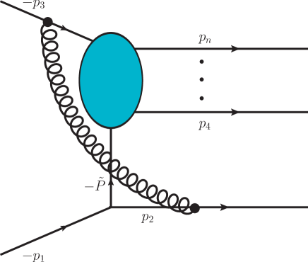
Figure 2: Two-parton SL collinear limit $(p_{i}\simeq z_{i}\widetilde{P},\;i=1,2)$ of the scattering amplitude ${\cal M}(p_{1},p_{2},p_{3},\dots,p_{n})$ with $n\geq 4$ QCD partons in parton–parton hard-scattering configurations. Typical (irreducible) colour structure of factorization breaking correlations at the one-loop level.

In hadron–hadron collisions (see Fig. 2), the SL collinear splitting of Eq. (20) takes place in a partonic environment that differs from that of lepton–hadron collisions. The main difference is due to the fact that the matrix element ${\cal M}(p_{1},p_{2},p_{3},\dots,p_{n})$ involves the initial-state collision of two QCD partons, the collinear parton with momentum $p_{1}$ and another parton, and both partons carry colour charge. The real part $\delta_{R}$ of the colour operator $\delta$ is the same as in Eq. (65) (see also Eq. (58)), while the imaginary part ${{\mbox{\boldmath$\delta$}}}_{I}$ is sensitive to the colour charge of the initial-state non-collinear parton. We assign the ‘outgoing’ momentum $p_{3}$ and the energy $p_{3}^{0}<0$ to this parton, and we can write the following explicit form of ${{\mbox{\boldmath$\delta$}}}_{I}$:

$${{\mbox{\boldmath$\delta$}}}_{I}(p_{1},p_{2};p_{3},..,p_{n})=+\;\frac{1}{\epsilon}\left\{\Bigl{(}C_{12}+C_{2}-C_{1}\Bigr{)}+4\;{{\mbox{\boldmath$T$}}}_{2}\cdot{{\mbox{\boldmath$T$}}}_{3}\right\}\;f_{I}(\epsilon;z_{2})\,,\;\;s_{23}<0<s_{j2}\;(j\geq 4)\,.$$ (66)

Combining this imaginary part with the real part (see Eq. (58)), the colour operator $\delta$ can be written in the following form:

$${{\mbox{\boldmath$\delta$}}}(p_{1},p_{2};p_{3},\dots,p_{n})=-\;\frac{1}{\epsilon}\;\Bigl{(}C_{12}+C_{2}-C_{1}\Bigr{)}\;f(\epsilon;z_{2}-i0)+\;\frac{i}{\epsilon}\;4\;{{\mbox{\boldmath$T$}}}_{2}\cdot{{\mbox{\boldmath$T$}}}_{3}\;f_{I}(\epsilon;z_{2})\;\;,$$ (67)

which clearly exhibits the difference with respect to the DIS expression in Eq. (65).

The expression in Eq. (66) is obtained from Eq. (59) by using simple colour algebra relations. Since $s_{23}<0$ and $s_{j2}>0\;(j\geq 4)$, the colour charge factor in Eq. (59) gives

$$-\;{{\mbox{\boldmath$T$}}}_{2}\cdot\left\{\sum_{j=3}^{n}\,{{\mbox{\boldmath$T$}}}_{j}\;{\rm sign}(s_{j2})\right\} = {{\mbox{\boldmath$T$}}}_{2}\cdot\left\{{{\mbox{\boldmath$T$}}}_{3}-\sum_{j=4}^{n}\,{{\mbox{\boldmath$T$}}}_{j}\right\}={{\mbox{\boldmath$T$}}}_{2}\cdot\left({{\mbox{\boldmath$T$}}}_{1}+{{\mbox{\boldmath$T$}}}_{2}+2\,{{\mbox{\boldmath$T$}}}_{3}\right)$$ (68)

$$= \frac{1}{2}\Bigl{(}C_{12}+C_{2}-C_{1}\Bigr{)}+2\;{{\mbox{\boldmath$T$}}}_{2}\cdot{{\mbox{\boldmath$T$}}}_{3}\;\;,$$

where we have used Eq. (38) (namely, $\sum_{j=4}^{n}\,{{\mbox{\boldmath$T$}}}_{j}=-({{\mbox{\boldmath$T$}}}_{1}+{{\mbox{\boldmath$T$}}}_{2}+{{\mbox{\boldmath$T$}}}_{3})$) and Eq. (42). Inserting Eq. (68) in Eq. (59), we get the result in Eq. (66).

The initial-state (hence, SL) collinear splitting in physical parton–parton scattering amplitudes ${\cal M}(p_{1},p_{2},\dots,p_{n})$ with $n\geq 4$ QCD partons necessarily involves colour correlations between the collinear and non-collinear partons. A representation of these correlations in minimal form is presented in the expression (66) of the imaginary part of the colour charge operator $\delta$ (see also Fig. 2).

4.5 Factorization, colour coherence and causality

The factorized structures of Eqs. (21) and (33) and, in particular, the violation of strict factorization in the case of SL collinear configurations deserve some physical (though qualitative) interpretation. We offer some comments about that.

The universal factorization of scattering amplitudes in the collinear limit is expected on the basis of a simple physical picture. When the two partons $A_{1}$ and $A_{2}$ with momenta $p_{1}$ and $p_{2}$ become collinear, their invariant mass $s_{12}$ is much smaller than $s_{j2}\sim s_{j1}$, where the subscript $j$ generically denotes a non-collinear parton $(j=3,4,\dots,n)$. Therefore, we are dealing with a two-scale process. Interactions between the collinear partons take place at the small energy scale $s_{12}$ and, hence, at large space-time distances; whereas, interactions between the non-collinear partons and interactions between the collinear and non-collinear partons require a large energy scale and, hence, they take place at small space-time distances. This space-time separation of large and small distances produces factorization. The (large-distance) physical subprocess $A\rightarrow A_{1}A_{2}$, which generates the collinear partons, is factorized from the (short-distance) scattering amplitude that involves the parent collinear parton $A$ and the non-collinear partons.

This simple space-time factorized picture is expressed, at the tree level, by the universal factorization formula in Eq. (9). At the one-loop (or higher-loop) level, the same space-time picture is too naïve, at least in the case of gauge theories. Owing to the long-range nature of gauge interactions, partonic fluctuations with arbitrarily-large wavelength (i.e. arbitrarily-small momentum) can propagate over widely-separated space-time regions, thus spoiling the factorization between the small-distance and large-distance subprocesses involved in the collinear limit.

To be more precise, we refer to one-loop interactions due to a gluon with soft momentum $q$ ($q\rightarrow 0)$. The soft gluon produces pairwise interactions between a collinear and a non-collinear parton. In the kinematical regions where the soft-gluon momentum has a very small angle with respect to the momentum of one of the external partons (either a collinear or a non-collinear parton), the one-loop interaction produces factorized (though IR divergent) contributions. Therefore, we are left to consider interactions due to a soft wide-angle gluon. Each of these pairwise interactions between a non-collinear $(j=3,4,\dots,n)$ and a collinear $(i=1,2)$ parton is proportional to the colour-charge term ${{\mbox{\boldmath$T$}}}_{j}\cdot{{\mbox{\boldmath$T$}}}_{i}\,$, and it is not factorized (it depends on the colour charge of both the non-collinear and collinear partons). These interactions separately spoil collinear factorization. Nonetheless, factorization can be recovered because of colour coherence.

The colour coherence mechanism that leads to factorization is as follows. We consider the kinematical region of wide-angle interaction. It is the region where $\theta_{jq}$ ($\theta_{jq}$ is the angle between $p_{j}$ and the soft momentum $q$) is large and, specifically, the region where $\theta_{jq}$ can reach values that are parametrically of the order of $\theta_{ji}$ ($\theta_{ji}$ is the angle between $p_{j}$ and the collinear momentum $p_{i}$). After integration over the soft-gluon momentum, the wide-angle interaction proportional to ${{\mbox{\boldmath$T$}}}_{j}\cdot{{\mbox{\boldmath$T$}}}_{1}\,$ depends on $\theta_{j1}$ and, analogously, the wide-angle interaction with the other collinear parton is proportional to ${{\mbox{\boldmath$T$}}}_{j}\cdot{{\mbox{\boldmath$T$}}}_{2}\,$ and depends on $\theta_{j2}$. In the collinear limit we have $\theta_{j1}=\theta_{j2}=\theta_{j\widetilde{P}}$ ($\widetilde{P}$ is the momentum of the parent parton) and, therefore, these two interaction contributions are combined in a single contribution that depends on $\theta_{j\widetilde{P}}$ and is proportional to the colour-charge term ${{\mbox{\boldmath$T$}}}_{j}\cdot({{\mbox{\boldmath$T$}}}_{1}+{{\mbox{\boldmath$T$}}}_{2})={{\mbox{\boldmath$T$}}}_{j}\cdot{{\mbox{\boldmath$T$}}}_{\widetilde{P}}\,$. This single contribution is exactly the contribution of the wide-angle interaction between the non-collinear parton $p_{j}$ and the parent parton $\widetilde{P}$: this contribution is factorized in the one-loop scattering amplitude $|{{\cal M}^{(1)}(\widetilde{P},\dots,p_{n})}\rangle$ on the right-hand side of Eqs. (21) and (33).

In summary, in the collinear limit the system of the two collinear partons acts coherently with respect to non-factorizable wide-angle interactions with each of the non-collinear partons. Owing to this coherent action, these interactions are removed from the collinear splitting matrix ${{\mbox{\boldmath$Sp$}}}^{(1)}$ and re-factorized in the matrix element $|{{\cal M}^{(1)}(\widetilde{P},\dots,p_{n})}\rangle$ of the factorization formulae (21) and (33).

The colour coherence mechanism that we have just illustrated is completely analogous to the mechanism that acts by considering the radiation of two collinear partons and a soft gluon in tree-level scattering amplitudes. In this mixed soft–collinear limit, the collinear splitting process is factorized from the soft-gluon current of the parent parton (see Sects. 3.4 and 3.5 in Ref. [11]). However, there is an essential difference between the radiation of a real gluon in tree-level amplitudes and the interactions of a virtual gluon in one-loop amplitudes. This difference is eventually responsible for the violation of strict factorization in the SL collinear limit of one-loop amplitudes.

A real gluon with soft momentum $q$ is always on-shell ($q^{2}=0$). A virtual gluon instead produces both a radiative (roughly speaking, real) and an absorptive (roughly speaking, imaginary) contribution to the one-loop amplitude. The radiative contribution is produced when the virtual soft gluon is on-shell ($q^{2}=0$), while the absorptive contribution is produced when the soft wide-angle gluon is slightly off-shell ($q^{2}\sim-{\bf q}_{\perp}^{2}$, where ${\bf q}_{\perp}$ is the gluon transverse momentum with respect to the direction of the momenta of the pair of interacting external partons).

The colour coherence phenomenon discussed so far in this subsection refers to the radiative part of the one-loop interactions. The absorptive (imaginary) part of the one-loop wide-angle interaction between the non-collinear parton $p_{j}$ and the collinear parton $p_{i}$ is very similar to its radiative part (it is still proportional to ${{\mbox{\boldmath$T$}}}_{j}\cdot{{\mbox{\boldmath$T$}}}_{i}\,$ and it simply depends on $\theta_{j\widetilde{P}}$ in the collinear limit), but it is non-vanishing only if $s_{ji}>0$ (as recalled below, this constraint follows from causality). Combining the absorptive part of the interactions of $p_{j}$ with the two collinear partons (as we did previously by combining the radiative part), we obtain a contribution that is proportional to ${{\mbox{\boldmath$T$}}}_{j}\cdot[\,{{\mbox{\boldmath$T$}}}_{1}\,\Theta(s_{j1})+{{\mbox{\boldmath$T$}}}_{2}\,\Theta(s_{j2})\,]$, and we see that the two collinear partons can act coherently only if their energies $p_{1}^{0}$ and $p_{2}^{0}$ have the same sign (i.e., in the case of the TL collinear limit). In the absence of this coherent action, the collinear splitting subprocess retains absorptive interactions with the non-collinear partons, and strict collinear factorization is violated in the SL collinear limit. In the generalized factorization formula (33), the amplitude $|{{\cal M}^{(1)}(\widetilde{P},\dots,p_{n})}\rangle$ includes the absorptive part of the interactions with the parent parton $\widetilde{P}$ (namely, the terms ${{\mbox{\boldmath$T$}}}_{j}\cdot\,{{\mbox{\boldmath$T$}}}_{\widetilde{P}}\;\Theta(s_{j\widetilde{P}})$), and the remaining absorptive contribution effectively included in ${{\mbox{\boldmath$Sp$}}}^{(1)}$ is proportional to

$${{\mbox{\boldmath$T$}}}_{j}\cdot\Bigl{[}\,{{\mbox{\boldmath$T$}}}_{1}\,\Theta(s_{j1})+{{\mbox{\boldmath$T$}}}_{2}\,\Theta(s_{j2})\,\Bigr{]}-{{\mbox{\boldmath$T$}}}_{j}\cdot\,{{\mbox{\boldmath$T$}}}_{\widetilde{P}}\;\Theta(s_{j\widetilde{P}})$$

$$={{\mbox{\boldmath$T$}}}_{j}\cdot\Bigl{[}\,{{\mbox{\boldmath$T$}}}_{1}\,\Bigl{(}\Theta(s_{j1})-\Theta(s_{j\widetilde{P}})\Bigr{)}+\,{{\mbox{\boldmath$T$}}}_{2}\,\Bigl{(}\Theta(s_{j2})-\Theta(s_{j\widetilde{P}})\Bigr{)}\,\Bigr{]}\;\;.$$

If, for example, we consider the SL case with $z_{2}<0$ (thus, $z_{1}>0$), the energies $s_{j1}$ and $s_{j\widetilde{P}}$ have the same sign, while the energies $s_{j2}$ and $s_{j\widetilde{P}}$ have opposite sign; the absorptive contribution to ${{\mbox{\boldmath$Sp$}}}^{(1)}$ is thus proportional to ${{\mbox{\boldmath$T$}}}_{j}\cdot\,{{\mbox{\boldmath$T$}}}_{2}\,\Bigl{(}\Theta(s_{j2})-\Theta(s_{j\widetilde{P}})\Bigr{)}={{\mbox{\boldmath$T$}}}_{j}\cdot\,{{\mbox{\boldmath$T$}}}_{2}\;{\rm sign}(s_{j2})$, which is exactly the colour-charge factor that appears in the right-hand side of Eq. (59).

The one-loop interaction between the partons $j$ and $i$ has a non-vanishing absorptive part only if the parton energies $p_{j}^{0}$ and $p_{i}^{0}$ have the same sign (i.e. only if $s_{ji}>0)$. This requires that the two partons belong to either the physical initial state or the physical final state of the scattering amplitude. In other words, the absorptive part has a definite causal structure (and origin): it arises from long-range interactions that takes place at large asymptotic times $t\rightarrow\pm\infty$, either in the past (considering initial-state partons) or in the future (considering final-state partons), with respect to the short time intervals that control the hard-scattering subprocess.

In gauge theories, factorization is potentially spoiled by the long-range nature of gauge interactions. Colour coherence can effectively restore the space-time factorization of small-distance and large-distance subprocesses. Colour coherence argument requires no distinctions between large space distances and large time distances. Causality does make distinctions between large distances at $t\rightarrow-\infty$ and $t\rightarrow+\infty$. Therefore, if the large-distance subprocess involves interactions at both $t\rightarrow-\infty$ and $t\rightarrow+\infty$ (as is the case of the two-parton collinear splitting in the SL region), the factorization power of colour coherence is limited by causality. This limitation leads to violation of ‘strict’ factorization.

The absorptive part of the one-loop splitting matrix ${{\mbox{\boldmath$Sp$}}}^{(1)}$ in Eq. (33) is responsible for violation of strict factorization in the SL collinear region. We observe that this absorptive part is IR divergent. Its IR divergent contribution (see e.g. Eq. (4.1) and remember that $f(\epsilon;z-i0)=-\ln(z-i0)+{\cal O}(\epsilon)$) is proportional to $-i\pi\,{{\mbox{\boldmath$T$}}}_{j}\cdot\,{{\mbox{\boldmath$T$}}}_{2}/\epsilon$, which exactly corresponds to the contribution of the non-abelian analogue of the QED Coulomb phase. It is well known (see, e.g., Refs. [37, 38, 39, 33, 30, 31, 32, 40, 41, 42] and references therein) that ‘Coulomb gluons’ lead to non-trivial QCD effects, especially in relation to various factorization issues and in connection with resummations of logarithmically-enhanced radiative corrections. Our study of the one-loop splitting matrix ${{\mbox{\boldmath$Sp$}}}^{(1)}(p_{1},p_{2};{\widetilde{P}};p_{3},\dots,p_{n})$ (including its absorptive part) is performed to all orders in the $\epsilon$ expansion. We thus note that our results on the SL collinear limit of two partons are not limited to the treatment of Coulomb gluon effects to leading IR (or logarithmic) accuracy.

5 Multiparton collinear limit and generalized factorization at one-loop order and beyond

5.1 Multiparton collinear limit of tree-level and one-loop amplitudes

The definition of the collinear limit of a set $\{p_{1},\dots,p_{m}\}$ of $m$ ($m\geq 3$) parton momenta follows the corresponding definition of the two-parton collinear limit (see Eqs. (2)–(5)). The multiparton collinear limit is approached when the momenta of the $m$ partons become parallel. This implies that all the parton subenergies

$$s_{i\ell}=(p_{i}+p_{\ell})^{2}\;\;,\quad\quad{\rm with}\;\;\;\;\;i,\ell\in C=\{\,1,\dots,m\,\}\;\;,$$ (69)

are of the same order and vanish simultaneously. In analogy with the two-parton collinear limit, we introduce the light-like momentum ${\widetilde{P}}^{\mu}$:

$${\widetilde{P}}^{\mu}=(p_{1}+\dots+p_{m})^{\mu}-\frac{(p_{1}+\dots+p_{m})^{2}\;n^{\mu}}{2\,n\cdot(p_{1}+\dots+p_{m})}\;\;.$$ (70)

In the multiparton collinear limit, the vector ${\widetilde{P}}^{\mu}$ approaches the collinear direction and we have $p_{i}^{\mu}\rightarrow z_{i}{\widetilde{P}}^{\mu}$, where the longitudinal-momentum fractions $z_{i}$ are

$$z_{i}=\frac{n\cdot p_{i}}{n\cdot{\widetilde{P}}}=\frac{n\cdot p_{i}}{n\cdot(p_{1}+\dots+p_{m})}\;\;,\quad\;\;\;i\in C\;\;,$$ (71)

and they fulfill the constraint $\sum_{i=1}^{m}z_{i}=1$. More details on the kinematics of the multiparton collinear limit can be found in Ref. [11].

As in the case of the two-parton collinear limit, the dynamics of the multiparton collinear limit of scattering amplitudes is different in the TL and SL regions. The TL region is specified by the constraints $s_{i\ell}=(p_{i}+p_{\ell})^{2}>0$, where $\{p_{i},p_{\ell}\}$ refers to any pair of collinear-parton momenta; note that these contraints imply $1>z_{i}>0$. If these contraints are not fulfilled, we are dealing with the SL region.

According to this definition, in the TL case, all the partons in the collinear set are either final-state partons (i.e., physically outgoing partons with ‘energies’ $p_{i}^{0}>0$) or initial-state partons (i.e., physically incoming partons with ‘energies’ $p_{i}^{0}<0$). In the SL case, the collinear set involves at least one parton in the initial state and, necessarily, one or more partons in the final state.

In the kinematical configuration where the $m$ parton momenta $p_{1},\dots,p_{m}$ become simultaneously parallel, the matrix element ${\cal M}={\cal M}(p_{1},\dots,p_{m},p_{m+1},\dots,p_{n})$ becomes singular. The dominant singular behaviour is ${\cal M}(p_{1},\dots,p_{m},p_{m+1},\dots,p_{n})\sim(1/{\sqrt{s}})^{m-1}\,{\rm mod\,}(\ln^{k}s)$ (see Eq. (6) for comparison), where the logarithmic enhancement is due to scaling violation that occurs through loop radiative corrections. Here $s$ denotes a generic two-parton (i.e., $s_{i\ell}$) or multiparton (e.g., $(p_{1}+p_{2}+p_{3})^{2}$) subenergy of the system of the $m$ collinear partons.

The extension of the collinear-factorization formulae (9), (21) and (33) to the case of the multiparton collinear limit is

$$|{{\cal M}^{(0)}}\rangle\simeq{{\mbox{\boldmath$Sp$}}}^{(0)}(p_{1},\dots,p_{m};{\widetilde{P}})\;\;|{{\overline{\cal M}}^{(0)}}\rangle\;\;,$$ (72)

$$|{{\cal M}^{(1)}}\rangle \simeq {{\mbox{\boldmath$Sp$}}}^{(1)}(p_{1},\dots,p_{m};{\widetilde{P}};p_{m+1},\dots,p_{n})\;\;|{{\overline{\cal M}}^{(0)}}\rangle$$ (73)

$$+ {{\mbox{\boldmath$Sp$}}}^{(0)}(p_{1},\dots,p_{m};{\widetilde{P}})\;\;|{{\overline{\cal M}}^{(1)}}\rangle\;\;.$$

On the right-hand side of Eqs. (72) and (73), we have neglected contributions that are subdominant (though, still singular) in the collinear limit, and we have denoted the ‘reduced’ matrix element by introducing the following shorthand notation:

$${\overline{\cal M}}={\cal M}(\widetilde{P},p_{m+1},\dots,p_{n})\;\;.$$ (74)

The reduced matrix element ${\overline{\cal M}}$ is obtained from the original matrix element ${\cal M}$ by replacing the $m$ collinear partons $A_{1},\dots,A_{m}$ (whose momenta are $p_{1},\dots,p_{m}$) with a single parton $A$, which carries the momentum $\widetilde{P}$. The flavour of the parent parton $A$ is determined by flavour conservation in the splitting subprocess $A\rightarrow A_{1}\dots A_{m}$.

The process dependence of the tree-level factorization formula (72) is entirely embodied in the matrix elements ${\cal M}$ and ${\overline{\cal M}}$. The splitting matrix ${{\mbox{\boldmath$Sp$}}}^{(0)}(p_{1},\dots,p_{m};{\widetilde{P}})$, which captures the dominant singular behaviour in the multiparton collinear limit, is universal (process independent). It depends on the momenta and quantum numbers (flavour, spin, colour) of the sole partons that are involved in the collinear splitting $A\rightarrow A_{1}\dots A_{m}$. The colour dependence can explicitly be denoted as (see Eq. (10) in the case of $m=2$ collinear partons)

$$Sp^{(0)\;(c_{1},\dots,c_{m};\,c)}(p_{1},\dots,p_{m};{\widetilde{P}})\equiv\langle{c_{1},\dots,c_{m}}|\;{{\mbox{\boldmath$Sp$}}}^{(0)}(p_{1},\dots,p_{m};{\widetilde{P}})\;|{c}\rangle\;\;,$$ (75)

where $c_{1},\dots,c_{m}$ are the colour indices of the partons $A_{1},\cdots,A_{m}$, and $c$ is the colour index of the parent parton $A$.

At the tree level, the TL and SL collinear limits have the same structure and are simply related by crossing symmetry relations. In going from the TL to the SL regions, the multiparton splitting matrix ${{\mbox{\boldmath$Sp$}}}^{(0)}(p_{1},\dots,p_{m};{\widetilde{P}})$ in Eq. (72) only varies because of the replacement of the wave function factors of the collinear partons (see the final part of Sect. 2). The dependence of ${{\mbox{\boldmath$Sp$}}}^{(0)}$ on the colours and momenta of the collinear partons is unchanged in the TL and SL regions.

At the one-loop order, the TL and SL collinear limits have a different structure. As a consequence of the violation of strict collinear factorization, Eq. (73) is presented in the form of generalized collinear factorization (see Eq. (33)). In the SL collinear region, the multiparton one-loop splitting matrix ${{\mbox{\boldmath$Sp$}}}^{(1)}$ also depends on the momenta and colour charges of the non-collinear partons in the matrix elements ${\cal M}$ and ${\overline{\cal M}}$. Introducing the colour dependence in explicit form, we have

$$\!\!\!\!\!\!\!\!Sp^{(1)\;(c_{1},\dots,c_{n};\,c,c_{m+1}^{\prime},\dots,c_{n}^{\prime})}(p_{1},\dots,p_{m};{\widetilde{P}};p_{m+1},\dots,p_{n})$$

$$\!\!\equiv\langle{c_{1},\dots,c_{n}}|\;{{\mbox{\boldmath$Sp$}}}^{(1)}(p_{1},\dots,p_{m};{\widetilde{P}};p_{m+1},\dots,p_{n})\;|{c,c_{m+1}^{\prime},\dots,c_{n}^{\prime}}\rangle\;\;,$$ (76)

where $c_{1},\dots,c_{n}$ are the colour indices of all (collinear and non-collinear) the external partons in the original matrix element ${\cal M}$, and $c,c_{m+1}^{\prime},\dots,c_{n}^{\prime}$ are the colour indices of all the external partons (i.e. the parent collinear parton and the non-collinear partons) in the reduced matrix element ${\overline{\cal M}}$. We remark that ${{\mbox{\boldmath$Sp$}}}^{(1)}$ does not depend on the spin polarization states of the non-collinear partons, since the violation of strict collinear factorization originates from soft interactions between the non-collinear and collinear partons (see Sect. 4.5). This origin of the violation of strict collinear factorization also implies that the one-loop multiparton splitting matrix ${{\mbox{\boldmath$Sp$}}}^{(1)}$ has factorization breaking terms with a linear dependence on the colour matrix of the non-collinear partons (see Eq. (4.1) and also Sect. 5.3). In the TL collinear region [28, 26] strict collinear factorization is recovered, and ${{\mbox{\boldmath$Sp$}}}^{(1)}$ is universal (i.e., independent of the non-collinear partons); thus, we can write:

$${{\mbox{\boldmath$Sp$}}}^{(1)}(p_{1},\dots,p_{m};{\widetilde{P}};p_{m+1},\dots,p_{n})={{\mbox{\boldmath$Sp$}}}^{(1)}(p_{1},\dots,p_{m};{\widetilde{P}})\;\;,\quad({\rm TL\,\;coll.\,\;lim.})\;\;,$$ (77)

where, precisely speaking, the notation means that ${{\mbox{\boldmath$Sp$}}}^{(1)}$ is proportional to the unit matrix in the colour subspace of the non-collinear partons.

As recalled in Sect. 2, collinear factorization of QCD amplitudes is usually presented in a colour-stripped formulation, which is obtained upon decomposition of the matrix element ${\cal M}$ in colour subamplitudes. In this formulation, the singular behaviour of the colour subamplitudes in the multiparton collinear limit is described by splitting amplitudes ${\rm Split}^{(0)}(p_{1},\dots,p_{m};{\widetilde{P}})$ (at the tree level) and ${\rm Split}^{(1)}$ (at the one-loop order). The splitting amplitudes can be regarded as matrices in helicity space, since they depend on the helicity states of the collinear partons. The splitting matrix $Sp$ in Eqs. (72) and (73) is a generalization of the splitting amplitude, since $Sp$ describes collinear factorization in colour+helicity space. In the case of the two-parton collinear limit, there is a straightforward direct proportionality (through a single colour matrix) between the splitting matrix ${{\mbox{\boldmath$Sp$}}}^{(0)}$ and the splitting amplitude ${\rm Split}^{(0)}$ (see Eq. (16)). Considering the collinear limit of $m$ partons, with $m\geq 3$, the corresponding splitting matrix ${{\mbox{\boldmath$Sp$}}}^{(0)}$ can get contributions from different colour structures. In general, ${{\mbox{\boldmath$Sp$}}}^{(0)}$ can be expressed as a linear combination of colour-matrix factors whose coefficients are kinematical splitting amplitudes ${\rm Split}^{(0)}$. Equivalently, the splitting amplitudes ${\rm Split}^{(0)}$ can be regarded (defined) as colour-stripped components of the splitting matrix ${{\mbox{\boldmath$Sp$}}}^{(0)}$. This correspondence between $Sp$ and ${\rm Split}$ functions extends from the tree-level to one-loop order in the TL collinear region. One-loop splitting amplitudes can be introduced also in the SL region (see Appendix A), by properly taking into account the violation of strict collinear factorization and the ensuing colour entanglement between collinear and non-collinear partons.

At the tree level, the multiparton $(m\geq 3)$ collinear limit has been extensively studied in the literature. In the case of $m=3$ collinear partons, explicit results for all QCD splitting processes $A\rightarrow A_{1}A_{2}A_{3}$ are known for both squared amplitudes [18, 19, 11] and amplitudes [20, 21, 22]. At the amplitude level, the multiparton collinear limit is explicitly known also in the cases of $m=4$ [20, 21] and $m=5$ and 6 [21] gluons. Considering some specific classes of helicity configurations of the collinear partons, the authors of Refs. [21, 22] derived general results for the splitting amplitude ${\rm Split}^{(0)}$ that are valid for an arbitrary number $m$ of gluons and of gluons plus up to four fermions $(q,q{\bar{q}},qq{\bar{q}},qq{\bar{q}}{\bar{q}})$.

At the one-loop level, the multiparton collinear limit in the TL region was studied in Ref. [26]: we explicitly computed the one-loop splitting matrix for the triple collinear limit $q\rightarrow q_{1}q_{2}^{\,\prime}{\bar{q}}_{3}^{\,\prime}$ ($q$ and $q^{\,\prime}$ are quarks with different flavour), and we presented the general structure of the IR and ultraviolet divergences of the one-loop splitting matrices. The latter result is recalled in Sect. 5.3, where it is also extended to the SL collinear region.

5.2 Generalized collinear factorization at all orders

The TL collinear limit of all-order QCD amplitudes is studied in Ref. [28], by using the unitarity sewing method [23, 43]. The detailed analysis of Ref. [28] is limited to the leading-colour terms, but it can be extended to subleading-colour contributions as shown by the explicit computations of splitting amplitudes at one-loop [25] and two-loop [27] orders. The collinear limit can be studied by using a different method [11] that relies on the factorization properties of Feynman diagrams in light-like axial gauges. By exploiting colour-coherence of QCD radiation, this method, which directly applies in colour space, can be extended [26] from tree-level to one-loop amplitudes in the TL collinear region. In Eq. (78), we propose an all-order factorization formula that is valid in both the TL and SL collinear regions. In the TL collinear limit, Eq. (78) represents a colour-space generalization of the all-order results of Ref. [28] or, similarly, an all-order generalization of the colour-space factorization of Refs. [11, 26]. The extension from the TL to the SL collinear regions is based on the generalized factorization structure (and the physical insight) that we have uncovered at the one-loop order (see Sects. 4 and 5.1). In Sect. 6, we show that Eq. (78) is consistent with the all-order factorization structure of the IR divergences of QCD amplitudes.

The generalized factorization formula for the multiparton collinear limit of the all-order matrix element ${\cal M}$ is

$$|{{\cal M}}\rangle\;\simeq\;{{\mbox{\boldmath$Sp$}}}(p_{1},\dots,p_{m};{\widetilde{P}};p_{m+1},\dots,p_{n})\;\;|{{\overline{\cal M}}}\rangle\;\;,$$ (78)

where $Sp$ is the all-order splitting matrix. The loop expansion of the unrenormalized splitting matrix is

$$\!\!\!\!\!\!\!\!\!\!\!\!\!{{\mbox{\boldmath$Sp$}}}(p_{1},\dots,p_{m};{\widetilde{P}};p_{m+1},\dots,p_{n})={{\mbox{\boldmath$Sp$}}}^{(0)}(p_{1},\dots,p_{m};{\widetilde{P}})$$

$$\!\!\!\!+\;{{\mbox{\boldmath$Sp$}}}^{(1)}(p_{1},\dots,p_{m};{\widetilde{P}};p_{m+1},\dots,p_{n})+{{\mbox{\boldmath$Sp$}}}^{(2)}(p_{1},\dots,p_{m};{\widetilde{P}};p_{m+1},\dots,p_{n})+\dots\;,$$ (79)

where ${{\mbox{\boldmath$Sp$}}}^{(1)}$ is its one-loop contribution, ${{\mbox{\boldmath$Sp$}}}^{(2)}$ is the two-loop splitting matrix, and so forth. The loop expansion of the matrix element ${\cal M}$ is defined in Eq. (1), and an analogous expression (it is obtained by simply replacing ${\cal M}^{(k)}$ with ${\overline{\cal M}}^{(k)}$) applies to the reduced matrix element ${\overline{\cal M}}$. Inserting these expansions in Eq. (78), we obtain factorization formulae that are valid order-by-order in the number of loops. At the tree level and one-loop order we recover Eqs. (72) and (73), respectively. The explicit factorization formula for the two-loop matrix element ${\cal M}^{(2)}$ is

$$|{{\cal M}^{(2)}}\rangle \simeq {{\mbox{\boldmath$Sp$}}}^{(2)}(p_{1},\dots,p_{m};{\widetilde{P}};p_{m+1},\dots,p_{n})\;\;|{{\overline{\cal M}}^{(0)}}\rangle$$ (80)

$$+ {{\mbox{\boldmath$Sp$}}}^{(1)}(p_{1},\dots,p_{m};{\widetilde{P}};p_{m+1},\dots,p_{n})\;\;|{{\overline{\cal M}}^{(1)}}\rangle$$

$$+ {{\mbox{\boldmath$Sp$}}}^{(0)}(p_{1},\dots,p_{m};{\widetilde{P}})\;\;|{{\overline{\cal M}}^{(2)}}\rangle\;\;.$$

In the case of the TL collinear limit, strict factorization is valid and the splitting matrix is process independent at each order in the loop expansion; we can remove the reference to the non-collinear partons, and we can simply write

$${{\mbox{\boldmath$Sp$}}}(p_{1},\dots,p_{m};{\widetilde{P}};p_{m+1},\dots,p_{n})={{\mbox{\boldmath$Sp$}}}(p_{1},\dots,p_{m};{\widetilde{P}})\;\;,\quad({\rm TL\,\;coll.\,\;lim.})\;\;.$$ (81)

Beyond the tree level, in the case of the SL collinear limit, the splitting matrix $Sp$ acquires also a dependence on the external non-collinear partons of ${\cal M}$ and ${\overline{\cal M}}$, although it is (expected to be) independent of the spin polarization states of these partons.

The all-order matrix elements ${\cal M}$ and ${\overline{\cal M}}$ in Eq. (78) are invariant under the renormalization procedure, since they are scattering amplitudes whose external partons are on-shell and with physical polarization states. Therefore, the splitting matrix $Sp$ (the remaining ingredient in Eq. (78)) is also invariant. The renormalization of ${\cal M},{\overline{\cal M}}$ and $Sp$ simply amounts to replace the bare coupling constant with the renormalized QCD coupling. The perturbative (loop) expansion with respect to the renormalized coupling is denoted as follows:

$${\cal M}={\cal M}^{(0,R)}+{\cal M}^{(1,R)}+{\cal M}^{(2,R)}+\dots\;\;,$$ (82)

$${{\mbox{\boldmath$Sp$}}}={{\mbox{\boldmath$Sp$}}}^{(0,R)}+{{\mbox{\boldmath$Sp$}}}^{(1,R)}+{{\mbox{\boldmath$Sp$}}}^{(2,R)}+\dots\;\;,$$ (83)

where the superscripts $(k,R)$ ($k=0,1,2,\dots$) refer to the renormalized expansions, whereas the superscripts $(k)$ refer to the unrenormalized expansions in the corresponding Eqs. (1) and (5.2). Since perturbative renormalization commutes with the collinear limit, the perturbative factorization formulae (72), (73) and (80) can equivalently be written by using the renormalized expansion. We simply have:

$$|{{\cal M}^{(0,R)}}\rangle \simeq {{\mbox{\boldmath$Sp$}}}^{(0,R)}\;|{{\overline{\cal M}}^{(0,R)}}\rangle\;\;,$$ (84)

$$|{{\cal M}^{(1,R)}}\rangle \simeq {{\mbox{\boldmath$Sp$}}}^{(1,R)}\;|{{\overline{\cal M}}^{(0,R)}}\rangle+{{\mbox{\boldmath$Sp$}}}^{(0,R)}\;|{{\overline{\cal M}}^{(1,R)}}\rangle\;\;,$$ (85)

$$|{{\cal M}^{(2,R)}}\rangle \simeq {{\mbox{\boldmath$Sp$}}}^{(2,R)}\;|{{\overline{\cal M}}^{(0,R)}}\rangle+{{\mbox{\boldmath$Sp$}}}^{(1,R)}\;|{{\overline{\cal M}}^{(1,R)}}\rangle+{{\mbox{\boldmath$Sp$}}}^{(0,R)}\;|{{\overline{\cal M}}^{(2,R)}}\rangle\;\;.$$ (86)

The main features of the results that we present in the following sections do not depend on the specific renormalization procedure. To avoid possible related ambiguities, we specify the renormalization (and regularization) procedure that we actually use in writing explicit expressions. The unrenormalized quantities are evaluated in $d=4-2\epsilon$ dimensions by using conventional dimensional regularization (CDR); in particular, the parton momenta are $d$ dimensional, and the gluon has $d-2=2-2\epsilon$ physical polarization states. The renormalized QCD coupling at the scale $\mu_{R}$ is denoted by $g_{\mathrm{S}}(\mu_{R}^{2})$ ($\alpha_{\mathrm{S}}=g_{\mathrm{S}}^{2}/(4\pi)$), and it is obtained from the unrenormalized (bare) coupling $g_{\mathrm{S}}$ by a modified minimal subtraction (${\overline{\rm MS}}$) procedure. We use the following explicit relation:

$$\mu^{2\,\epsilon}\,g_{\mathrm{S}}^{2}\;S_{\epsilon}=\mu_{R}^{2\,\epsilon}\;g_{\mathrm{S}}^{2}(\mu_{R}^{2})\left[1-\frac{\alpha_{\mathrm{S}}(\mu_{R}^{2})}{2\pi}\;\frac{b_{0}}{\epsilon}+\left(\frac{\alpha_{\mathrm{S}}(\mu_{R}^{2})}{2\pi}\right)^{2}\left(\frac{b_{0}^{2}}{\epsilon^{2}}-\frac{b_{1}^{2}}{2\epsilon}\right)+{\cal O}(\alpha_{\mathrm{S}}^{3}(\mu_{R}^{2}))\right]\;\,,$$ (87)

where $S_{\epsilon}$ is the customary ${\overline{\rm MS}}$ factor ($\gamma_{E}=-\psi(1)=0.5772\dots$ is the Euler number),

$$S_{\epsilon}=\exp\left[\,\epsilon\,(\ln 4\pi+\psi(1))\right]\;\;,$$ (88)

and $b_{0}$ (see Eq. (32)) and $b_{1}$ are the first two coefficients of the QCD $\beta$ function, with

$$b_{1}=(17\,C_{A}^{2}-5\,C_{A}N_{f}-3\,C_{F}N_{f})/6\;\;.$$ (89)

In the following, all the renormalized expressions refer to the perturbative expansion with respect to $\alpha_{\mathrm{S}}(\mu^{2})$ (i.e., the renormalization scale $\mu_{R}$ is always set to be equal to the dimensional-regularization scale $\mu$). For instance, considering the splitting matrix $Sp$ of $m$ collinear partons, the tree-level and one-loop relations between the renormalized (see Eq. (83)) and unrenormalized (see Eq. (5.2)) contributions are as follows:

$${{\mbox{\boldmath$Sp$}}}^{(0,R)}=\left[{{\mbox{\boldmath$Sp$}}}^{(0)}\right]_{g_{\mathrm{S}}=g_{\mathrm{S}}(\mu^{2})S_{\epsilon}^{\,-\frac{1}{2}}}\;\;,$$ (90)

$${{\mbox{\boldmath$Sp$}}}^{(1,R)}=-\,\frac{\alpha_{\mathrm{S}}(\mu^{2})}{2\pi}\;\frac{m-1}{2}\;\frac{b_{0}}{\epsilon}\;{{\mbox{\boldmath$Sp$}}}^{(0,R)}\,+\left[{{\mbox{\boldmath$Sp$}}}^{(1)}\right]_{g_{\mathrm{S}}=g_{\mathrm{S}}(\mu^{2})S_{\epsilon}^{\,-\frac{1}{2}}}\;\;.$$ (91)

The first term on the right-hand side of Eq. (91) originates from the fact that the corresponding tree-level contribution ${{\mbox{\boldmath$Sp$}}}^{(0)}$ is proportional to $g_{\mathrm{S}}^{m-1}$.

In the case of the two-parton collinear limit, for later purposes, we can write the renormalized version of Eq. (4.1) in the following form:

$${{\mbox{\boldmath$Sp$}}}^{(1,R)}(p_{1},p_{2};{\widetilde{P}};p_{3},\dots,p_{n})={\widetilde{{\mbox{\boldmath$I$}}}}_{C}^{(1)}(\epsilon)\;{{\mbox{\boldmath$Sp$}}}^{(0,R)}(p_{1},p_{2};{\widetilde{P}})+{{\mbox{\boldmath$Sp$}}}^{(1,R)}_{H}(p_{1},p_{2};{\widetilde{P}})\;,$$ (92)

$${\widetilde{{\mbox{\boldmath$I$}}}}_{C}^{(1)}(\epsilon) = \frac{\alpha_{\mathrm{S}}(\mu^{2})}{2\pi}\;\frac{1}{2}\;\,{\widetilde{c}}_{\Gamma}\left(\frac{-s_{12}-i0}{\mu^{2}}\right)^{-\epsilon}$$ (93)

$$\times \left\{\;\frac{1}{\epsilon^{2}}\;\Bigl{(}C_{12}-C_{1}-C_{2}\Bigr{)}+\frac{1}{\epsilon}\;\Bigl{(}\gamma_{12}-\gamma_{1}-\gamma_{2}\Bigr{)}\right.$$

$$- \left.\;\frac{1}{\epsilon}\,\left[\Bigl{(}C_{12}+C_{1}-C_{2}\Bigr{)}\;f_{R}(\epsilon;z_{1})+\Bigl{(}C_{12}+C_{2}-C_{1}\Bigr{)}\;f_{R}(\epsilon;z_{2})\;\right]\right.$$

$$- \;\;i\left.\,\frac{2}{\epsilon}\;\sum_{j=3}^{n}\,\sum_{i=1,2}\,{{\mbox{\boldmath$T$}}}_{j}\cdot{{\mbox{\boldmath$T$}}}_{i}\;\,{\rm sign}(s_{ij})\;\,\Theta(-z_{i})\;\,f_{I}(\epsilon;z_{i})\;\right\}\;\;,$$

where the coefficient ${\widetilde{c}}_{\Gamma}=1+{\cal O}(\epsilon^{2})$ is related to the volume factor $c_{\Gamma}$ in Eq. (30) and it is defined as

$${\widetilde{c}}_{\Gamma}\equiv\left(4\pi\right)^{2}\;S_{\epsilon}^{-1}\;c_{\Gamma}=\frac{\Gamma(1+\epsilon)\,\Gamma^{2}(1-\epsilon)}{\Gamma(1-2\epsilon)}\;e^{-\epsilon\,\psi(1)}\;\;\;.$$ (94)

The colour operator ${\widetilde{{\mbox{\boldmath$I$}}}}_{C}^{(1)}(\epsilon)$ is directly related to the corresponding unrenormalized operator ${{\mbox{\boldmath$I$}}}_{C}(p_{1},p_{2};p_{3},\dots,p_{n})$ (the functional dependence on the parton momenta is not explicitly recalled in the argument of ${\widetilde{{\mbox{\boldmath$I$}}}}_{C}^{(1)}$) in Eq. (4.1). In the expression on the right-hand side of Eq. (93), the colour correlation contributions proportional to ${{\mbox{\boldmath$T$}}}_{j}\cdot{{\mbox{\boldmath$T$}}}_{i}$ are written as in Eqs. (56)–(59), by using the decomposition of $f(\epsilon;z)$ in its real and imaginary parts. We also note that the contribution proportional to $b_{0}$ in ${{\mbox{\boldmath$I$}}}_{C}$ and the renormalization counterterm of ${{\mbox{\boldmath$Sp$}}}^{(1,R)}$ (i.e. the first term on the right-hand side of Eq. (91)) have been included in the definition of ${{\mbox{\boldmath$Sp$}}}^{(1,R)}_{H}$. Thus, in Eq. (92), ${{\mbox{\boldmath$Sp$}}}^{(1,R)}_{H}$ has been defined as

$${{\mbox{\boldmath$Sp$}}}^{(1,R)}_{H}(p_{1},p_{2};{\widetilde{P}}) \equiv \frac{\alpha_{\mathrm{S}}(\mu^{2})}{2\pi}\;\frac{b_{0}}{2\epsilon}\left[\,{\widetilde{c}}_{\Gamma}\left(\frac{-s_{12}-i0}{\mu^{2}}\right)^{-\epsilon}-1\right]\;{{\mbox{\boldmath$Sp$}}}^{(0,R)}(p_{1},p_{2};{\widetilde{P}})$$ (95)

$$+ \left[{{\mbox{\boldmath$Sp$}}}^{(1)}_{H}(p_{1},p_{2};{\widetilde{P}})\right]_{g_{\mathrm{S}}=g_{\mathrm{S}}(\mu^{2})S_{\epsilon}^{\,-\frac{1}{2}}}\;\;\;\;.$$

The first term on the right-hand side is finite when $\epsilon\rightarrow 0$, since the ultraviolet divergence of ${{\mbox{\boldmath$I$}}}_{C}$ is cancelled by the renormalization of the one-loop splitting matrix. The remaining $\epsilon$ poles of ${{\mbox{\boldmath$Sp$}}}^{(1,R)}$ are of IR origin, and they are included in the colour operator ${\widetilde{{\mbox{\boldmath$I$}}}}_{C}^{(1)}(\epsilon)$.

5.3 The IR divergences of the one-loop splitting matrix

Analogously to the case of two-collinear partons, the one-loop splitting matrix ${{\mbox{\boldmath$Sp$}}}^{(1,R)}$ of the multiparton collinear limit in Eq. (85) (or Eq. (73)) has IR divergences. They show up as double $(1/\epsilon^{2})$ and single $(1/\epsilon)$ poles in the expansion around the point $\epsilon=0$. To make the IR behaviour explicit, we separate the divergent and finite terms as follows:

$${{\mbox{\boldmath$Sp$}}}^{(1,R)}={{\mbox{\boldmath$Sp$}}}^{(1)\,{\rm div.}}+{{\mbox{\boldmath$Sp$}}}^{(1)\,{\rm fin.}}\;\;,$$ (96)

where ${{\mbox{\boldmath$Sp$}}}^{(1)\,{\rm div.}}$ contains the $\epsilon$ poles, while ${{\mbox{\boldmath$Sp$}}}^{(1)\,{\rm fin.}}$ is finite when $\epsilon\rightarrow 0$. Then, we can present our general result for the IR divergent part.

The computation of the divergent part shows that it can be written in a colour-space factorized form:

$${{\mbox{\boldmath$Sp$}}}^{(1)\,{\rm div.}}(p_{1},\dots,p_{m};{\widetilde{P}};p_{m+1},\dots,p_{n})={{\mbox{\boldmath$I$}}}^{(1)}_{m\,C}(\epsilon)\;\,{{\mbox{\boldmath$Sp$}}}^{(0,R)}(p_{1},\dots,p_{m};{\widetilde{P}})\;\;,$$ (97)

where ${{\mbox{\boldmath$Sp$}}}^{(0,R)}$ is the tree-level splitting matrix, including its complete (i.e. exact) dependence on $\epsilon$. The colour space operator ${{\mbox{\boldmath$I$}}}^{(1)}_{m\,C}$ depends on the collinear partons and, in the SL region, it also depends on the momenta and colour charges of the non-collinear partons in the original matrix element ${\cal M}$. Analogously to the notation in Eq. (92), the functional dependence on all partons is not explicitly denoted in the argument of ${{\mbox{\boldmath$I$}}}^{(1)}_{m\,C}$. We present ${{\mbox{\boldmath$I$}}}^{(1)}_{m\,C}$ in a general form, which is valid in both the SL and TL collinear limits. Considering the collinear splitting process $A\rightarrow A_{1}\dots A_{m}$, the explicit expression of ${{\mbox{\boldmath$I$}}}^{(1)}_{m\,C}$ is

$${{\mbox{\boldmath$I$}}}^{(1)}_{m\,C}(\epsilon) = \frac{\alpha_{\mathrm{S}}(\mu^{2})}{2\pi}\;\frac{1}{2}\;\left\{\left(\,\frac{1}{\epsilon^{2}}\,C_{\widetilde{P}}+\frac{1}{\epsilon}\,\gamma_{\widetilde{P}}\right)-\sum_{\begin{subarray}{c}i\,\in\,C\\ {}\end{subarray}}\left(\,\frac{1}{\epsilon^{2}}\,C_{i}+\frac{1}{\epsilon}\,\gamma_{i}\right)\right.$$ (98)

$$- \frac{1}{\epsilon}\sum_{\begin{subarray}{c}i,\ell\,\in C\\ i\,\neq\,\ell\end{subarray}}{{\mbox{\boldmath$T$}}}_{i}\cdot{{\mbox{\boldmath$T$}}}_{\ell}\,\ln\left(\frac{-s_{i\ell}-i0}{\mu^{2}}\right)\left.-\;\frac{2}{\epsilon}\sum_{\begin{subarray}{c}i\,\in C\\ j\,\in NC\end{subarray}}{{\mbox{\boldmath$T$}}}_{i}\cdot{{\mbox{\boldmath$T$}}}_{j}\,\ln\bigl{(}z_{i}-i0s_{ij}\bigr{)}\right\}\;,$$

where the subscript ${\widetilde{P}}$ refers to the parent collinear parton $A$. The sets

$$C=\{1,\dots,m\}\quad{\rm and}\quad NC=\{m+1,\dots,n\}$$

denote the collinear and non-collinear partons, respectively.

The expression (98) can be written in the following equivalent form:

$${{\mbox{\boldmath$I$}}}^{(1)}_{m\,C}(\epsilon) = \frac{\alpha_{\mathrm{S}}(\mu^{2})}{2\pi}\;\frac{1}{2}\;\left\{\left(\,\frac{1}{\epsilon^{2}}\,C_{\widetilde{P}}+\frac{1}{\epsilon}\,\gamma_{\widetilde{P}}\right)-\sum_{\begin{subarray}{c}i\,\in\,C\\ {}\end{subarray}}\left(\,\frac{1}{\epsilon^{2}}\,C_{i}+\frac{1}{\epsilon}\,\gamma_{i}-\,\frac{2}{\epsilon}\,C_{i}\,\ln|z_{i}|\right)\right.$$ (99)

$$- \frac{1}{\epsilon}\left.\sum_{\begin{subarray}{c}i,\ell\,\in C\\ i\,\neq\,\ell\end{subarray}}{{\mbox{\boldmath$T$}}}_{i}\cdot{{\mbox{\boldmath$T$}}}_{\ell}\,\ln\left(\frac{-s_{i\ell}-i0}{|z_{i}|\,|z_{\ell}|\,\mu^{2}}\right)\right\}+{{\mbox{\boldmath$\Delta$}}}^{(1)}_{m\,C}(\epsilon)\;\;,$$

where

$${{\mbox{\boldmath$\Delta$}}}^{(1)}_{m\,C}(\epsilon)=\frac{\alpha_{\mathrm{S}}(\mu^{2})}{2\pi}\,\;\frac{i\pi}{\epsilon}\;\sum_{\begin{subarray}{c}i\,\in C\\ j\,\in NC\end{subarray}}{{\mbox{\boldmath$T$}}}_{i}\cdot{{\mbox{\boldmath$T$}}}_{j}\;\Theta(-z_{i})\;{\rm sign}(s_{ij})\;\;.$$ (100)

The result in Eq. (98) (or Eq. (99)) contains double and single poles in $1/\epsilon$. For the specific case of $m=2$ collinear partons, this result agrees with the $\epsilon$ poles of the complete one-loop result in Eqs. (92) and (93). In the general case of $m$ collinear partons, we can see that ${{\mbox{\boldmath$I$}}}^{(1)}_{m\,C}$ embodies colour-correlation terms that produce violation of strict collinear factorization. In the expression (99), these correlations are fully taken into account by the colour operator ${{\mbox{\boldmath$\Delta$}}}^{(1)}_{m\,C}(\epsilon)$. The expression (100) explicitly shows that the operator ${{\mbox{\boldmath$\Delta$}}}^{(1)}_{m\,C}$ is antihermitian. In particular, ${{\mbox{\boldmath$\Delta$}}}^{(1)}_{m\,C}(\epsilon)$ is proportional to a single pole $1/\epsilon$ and exactly corresponds to the colour-correlation terms that are produced by the non-abelian Coulomb phase (see Sect. 4.5).

The computation of the finite part of Eq. (96), in the case of the SL collinear limit of $m=3$ partons, is in progress. In general, we can anticipate that ${{\mbox{\boldmath$Sp$}}}^{(1)\,{\rm fin.}}$ also contains factorization breaking contributions, and they are of the same type as those in ${{\mbox{\boldmath$\Delta$}}}^{(1)}_{m\,C}$, namely, they have the form of two-parton correlations ${{\mbox{\boldmath$T$}}}_{i}\cdot{{\mbox{\boldmath$T$}}}_{j}$ with $i\in C$ and $j\in NC$.

In the TL collinear region, the longitudinal-momentum fractions $z_{i}$ are positive. Therefore, ${{\mbox{\boldmath$\Delta$}}}^{(1)}_{m\,C}$ vanishes and the result in Eq. (99) has a strict-factorization form, which agrees with the result in Eq. (11) of Ref. [26]. To be precise, Eq. (11) of Ref. [26] contains an additional single pole of UV origin (that expression refers to the unrenormalized splitting matrix) and additional IR finite terms, which include the ${\cal O}(\epsilon^{0})$ terms of ${{\mbox{\boldmath$Sp$}}}^{(1)}$ that explicitly depend on the regularization scheme. In the TL collinear region, the expression (99) can also be rewritten in a slightly-simpler form, as follows:

$$\!\!\!\!\!\!\!\!\!\!\!\!{{\mbox{\boldmath$I$}}}^{(1)}_{m\,C}(\epsilon) = \frac{\alpha_{\mathrm{S}}(\mu^{2})}{2\pi}\;\frac{1}{2}\;\left\{\left(\,\frac{1}{\epsilon^{2}}\,C_{\widetilde{P}}+\frac{1}{\epsilon}\,\gamma_{\widetilde{P}}\right)-\sum_{\begin{subarray}{c}i\,\in\,C\\ {}\end{subarray}}\left(\,\frac{1}{\epsilon^{2}}\,C_{i}+\frac{1}{\epsilon}\,\gamma_{i}-\,\frac{2}{\epsilon}\,C_{i}\,\ln z_{i}\right)\right.$$ (101)

$$- \frac{1}{\epsilon}\sum_{\begin{subarray}{c}i,\ell\,\in C\\ i\,\neq\,\ell\end{subarray}}{{\mbox{\boldmath$T$}}}_{i}\cdot{{\mbox{\boldmath$T$}}}_{\ell}\,\ln\left(\frac{s_{i\ell}}{z_{i}z_{\ell}\,\mu^{2}}\right)\left.+\;\frac{i\pi}{\epsilon}\left(\,C_{\widetilde{P}}-\sum_{i\,\in\,C}\,C_{i}\right)\right\}\;,\;\;({\rm TL\,\;coll.\,\;lim.})\,.$$

We can see that the antihermitian part of ${{\mbox{\boldmath$I$}}}^{(1)}_{m\,C}$ is simply an imaginary $c$-number. Therefore, in the TL collinear limit, the non-abelian Coulomb phase effectively takes an abelian form.

The derivation of the results in Eqs. (97) and (98) is presented below. As for the rewriting in Eqs. (99) and (101), it simply follows from colour conservation properties. Considering the last term on the right-hand side of Eq. (98), we can write $\ln\bigl{(}z_{i}-i0s_{ij}\bigr{)}=\ln|z_{i}|-i\pi\Theta(-z_{i})\;{\rm sign}(s_{ij})$ and then, using the conservation of the total colour charge,

$$\sum_{j\,\in NC}\;{{\mbox{\boldmath$T$}}}_{j}=-\sum_{i\,\in C}\;{{\mbox{\boldmath$T$}}}_{i}\;\;,$$ (102)

we directly obtain Eqs. (99) and (100). Considering the last term in the curly bracket on the right-hand side of Eq. (99), we can write $\ln(-s_{i\ell}-i0)=\ln s_{i\ell}-i\pi$ ($s_{i\ell}>0$ in the TL collinear region), and then Eq. (101) is directly obtained by using $\;\sum_{i,\ell\,\in C}{{\mbox{\boldmath$T$}}}_{i}\cdot{{\mbox{\boldmath$T$}}}_{\ell}=C_{\widetilde{P}}$ or, more precisely, by using the relation

$$\Bigl{(}\;\sum_{i\,\in C}{{\mbox{\boldmath$T$}}}_{i}\;\Bigr{)}\;{{\mbox{\boldmath$Sp$}}}^{(0,R)}={{\mbox{\boldmath$Sp$}}}^{(0,R)}\;{{\mbox{\boldmath$T$}}}_{\widetilde{P}}\;\;.$$ (103)

This relation (which generalizes Eq. (40) to the case of $m$ collinear partons) follows from the fact that the colour charge ${{\mbox{\boldmath$T$}}}_{\widetilde{P}}$ of the parent parton $A$ is conserved in the tree-level collinear splitting $A\rightarrow A_{1}\dots A_{m}$.

Note that, in the case of the TL collinear splitting, Eq. (103) remains valid when replacing the tree-level splitting matrix ${{\mbox{\boldmath$Sp$}}}^{(0,R)}$ with the all-order splitting matrix $Sp$. We remark that this all-order generalization does not apply to the SL collinear limit. In the SL case, owing to the violation of strict factorization, ${{\mbox{\boldmath$Sp$}}}^{(1)}$, ${{\mbox{\boldmath$Sp$}}}^{(2)}$ and so forth, contain charge interactions between collinear and non-collinear partons: therefore, only their total charge is conserved (and the equality in (103) is not valid beyond the tree level).

The results in Eqs. (97) and (98) can be derived in a simple way by exploiting the known IR structure of generic one-loop QCD amplitudes [47, 35, 1]. Considering the scattering amplitude ${\cal M}$ with $n$ external QCD partons (and any number of colourless external legs), the renormalized one-loop contribution can be written in the following factorized form [1]:

$$|{{\cal M}^{(1,R)}}\rangle={{\mbox{\boldmath$I$}}}^{(1)}_{M}(\epsilon)\;|{{\cal M}^{(0,R)}}\rangle+\;|{{\cal M}^{(1)\,{\rm fin.}}}\rangle\;\;,$$ (104)

where

$${{\mbox{\boldmath$I$}}}^{(1)}_{M}(\epsilon)=\frac{\alpha_{\mathrm{S}}(\mu^{2})}{2\pi}\;\frac{1}{2}\;\Bigl{\{}\;-\sum_{i=1}^{n}\left(\frac{1}{\epsilon^{2}}\,C_{i}+\frac{1}{\epsilon}\,\gamma_{i}\right)-\frac{1}{\epsilon}\sum_{\begin{subarray}{c}i,j=1\\ i\neq j\end{subarray}}^{n}\;{{\mbox{\boldmath$T$}}}_{i}\cdot{{\mbox{\boldmath$T$}}}_{j}\,\ln\left(\frac{-s_{ij}-i0}{\mu^{2}}\right)\;\Bigr{\}}\;\;,$$ (105)

and the one-loop term $|{{\cal M}^{(1)\,{\rm fin.}}}\rangle$ is finite when $\epsilon\rightarrow 0$. The singular dependence on $\epsilon$ is embodied in the factor ${{\mbox{\boldmath$I$}}}^{(1)}_{M}(\epsilon)$ that acts as a colour-charge operator onto the tree-level matrix element $|{{\cal M}^{(0,R)}}\rangle$ (which retains its complete dependence on $\epsilon$). The colour operator ${{\mbox{\boldmath$I$}}}^{(1)}_{M}$ is equivalent, though it is not exactly equal, to the operator ${{\mbox{\boldmath$I$}}}^{(1)}$ introduced in Ref. [1]; the expression (105) is obtained from ${{\mbox{\boldmath$I$}}}^{(1)}$ by removing all terms that are finite at $\epsilon=0$ (these terms are absorbed in the definition of $|{{\cal M}^{(1)\,{\rm fin.}}}\rangle$).

The universality structure of the IR factorization formulae (104) and (105) has direct consequences on the collinear limit of the scattering amplitudes. Indeed, Eq. (104) can be applied to the matrix element ${\cal M}$ before performing the collinear limit, and an analogous relation (which is obtained by the replacements ${\cal M}\rightarrow{\overline{\cal M}}$ and ${{\mbox{\boldmath$I$}}}^{(1)}_{M}\rightarrow{{\mbox{\boldmath$I$}}}^{(1)}_{{\overline{M}}}\,$) applies to the reduced matrix element ${\overline{\cal M}}$. Therefore, we have:

$$\!\!\!\!\!\!\!\!\!\!\!\!\!\!\!\!\!\!\!\!\!\!\!{{\mbox{\boldmath$Sp$}}}^{(1,R)}\;|{{\overline{\cal M}}^{(0,R)}}\rangle\simeq\;|{{\cal M}^{(1,R)}}\rangle-\,{{\mbox{\boldmath$Sp$}}}^{(0,R)}\;|{{\overline{\cal M}}^{(1,R)}}\rangle$$ (106)

$$\!\!\!\!= \!\!\!\!\!\!{{\mbox{\boldmath$I$}}}^{(1)}_{M}(\epsilon)\;|{{\cal M}^{(0,R)}}\rangle-\,{{\mbox{\boldmath$Sp$}}}^{(0,R)}\;{{\mbox{\boldmath$I$}}}^{(1)}_{{\overline{M}}}(\epsilon)\;|{{\overline{\cal M}}^{(0,R)}}\rangle+\;|{{\cal M}^{(1)\,{\rm fin.}}}\rangle-\,{{\mbox{\boldmath$Sp$}}}^{(0,R)}\;|{{\overline{\cal M}}^{(1)\,{\rm fin.}}}\rangle$$ (107)

$$\!\!\!\!\simeq \!\!\!\!\!\!\left({{\mbox{\boldmath$I$}}}^{(1)}_{M}(\epsilon)\;{{\mbox{\boldmath$Sp$}}}^{(0,R)}-\,{{\mbox{\boldmath$Sp$}}}^{(0,R)}\;{{\mbox{\boldmath$I$}}}^{(1)}_{{\overline{M}}}(\epsilon)\right)\;|{{\overline{\cal M}}^{(0,R)}}\rangle+\;|{{\cal M}^{(1)\,{\rm fin.}}}\rangle-\,{{\mbox{\boldmath$Sp$}}}^{(0,R)}\;|{{\overline{\cal M}}^{(1)\,{\rm fin.}}}\rangle\,.$$ (108)

Equation (106) is just a rewriting of the one-loop collinear factorization in Eq. (85). Then, Eq. (107) is obtained by using Eq. (104) for both ${\cal M}^{(1,R)}$ and ${\overline{\cal M}}^{(1,R)}$. Finally, Eq. (108) is obtained by applying the tree-level factorization formula (84) to ${\cal M}^{(0,R)}$. Performing these steps, we have only neglected subdominant collinear terms (as denoted by the approximate equalities in Eq. (106) and (108)). The last terms, $|{{\cal M}^{(1)\,{\rm fin.}}}\rangle$ and ${{\mbox{\boldmath$Sp$}}}^{(0,R)}\;|{{\overline{\cal M}}^{(1)\,{\rm fin.}}}\rangle$, on the right-hand side of Eq. (108) do not contain any $\epsilon$ poles, and they are finite if $\epsilon\rightarrow 0$. Thus, in the collinear limit, we can write

$${{\mbox{\boldmath$Sp$}}}^{(1,R)}\;\simeq\;{{\mbox{\boldmath$I$}}}^{(1)}_{M}(\epsilon)\;{{\mbox{\boldmath$Sp$}}}^{(0,R)}-\,{{\mbox{\boldmath$Sp$}}}^{(0,R)}\;{{\mbox{\boldmath$I$}}}^{(1)}_{{\overline{M}}}(\epsilon)\;+\;{\cal O}(\epsilon^{0})\;\;.$$ (109)

The IR divergent contributions in Eqs. (97) and (98) directly derive from the relation (109), by simply using colour-charge conservation. To illustrate the derivation in detail, we note that, according to Eq. (105), the operator $\;{{\mbox{\boldmath$I$}}}^{(1)}_{M}$ on the right-hand side of Eq. (109) contains three classes of contributions: $(a)$ terms that only depend on the non-collinear partons; $(b)$ terms that only depend on the collinear partons in ${\cal M}$; $(c)$ terms that depend on both the collinear and non-collinear partons. Correspondingly, the operator $\;{{\mbox{\boldmath$I$}}}^{(1)}_{{\overline{M}}}$ contains the following classes of contributions: $({\overline{a}})$ terms that only depend on the non-collinear partons; $({\overline{b}})$ terms that only depend on the parent collinear parton $A$ in ${\overline{\cal M}}$; $({\overline{c}})$ terms that depend on both the parent parton and the non-collinear partons. The terms of the classes $(a)$ and $({\overline{a}})$ are exactly equal and commute with ${{\mbox{\boldmath$Sp$}}}^{(0,R)}$: therefore, they cancel on the right-hand side of Eq. (109). The terms of the class $({\overline{b}})$ are proportional to either $C_{\widetilde{P}}$ or $\gamma_{\widetilde{P}}$; they commute with ${{\mbox{\boldmath$Sp$}}}^{(0,R)}$ and combine with the terms of the class $(b)$, thus leading to the first three contributions in the curly bracket of Eq. (98). The last contribution (which depends on ${{\mbox{\boldmath$T$}}}_{i}\cdot{{\mbox{\boldmath$T$}}}_{j}$) in the curly bracket of Eq. (98) is due to the terms of the remaining classes $(c)$ and $({\overline{c}})$. Indeed, these terms give the following contribution to the right-hand side of Eq. (109) (we omit an overall factor of $\alpha_{\mathrm{S}}/(4\pi)$ and use the notation $s_{j\widetilde{P}}=2p_{j}\cdot{\widetilde{P}}$):

$$-\,\frac{2}{\epsilon}\sum_{\begin{subarray}{c}i\,\in C\\ j\,\in NC\end{subarray}}\;{{\mbox{\boldmath$T$}}}_{j}\cdot{{\mbox{\boldmath$T$}}}_{i}\,\ln\left(\frac{-s_{ji}-i0}{\mu^{2}}\right)\;{{\mbox{\boldmath$Sp$}}}^{(0,R)}+{{\mbox{\boldmath$Sp$}}}^{(0,R)}\;\frac{2}{\epsilon}\sum_{j\,\in NC}\;{{\mbox{\boldmath$T$}}}_{j}\cdot{{\mbox{\boldmath$T$}}}_{\widetilde{P}}\,\ln\left(\frac{-s_{j\widetilde{P}}-i0}{\mu^{2}}\right)$$

(110)

$$\simeq-\,\frac{2}{\epsilon}\sum_{\begin{subarray}{c}i\,\in C\\ j\,\in NC\end{subarray}}\;{{\mbox{\boldmath$T$}}}_{j}\cdot{{\mbox{\boldmath$T$}}}_{i}\,\ln\left(z_{i}-i0s_{ji}\right)\;{{\mbox{\boldmath$Sp$}}}^{(0,R)}$$

$$\;\;\;\;-\,\frac{2}{\epsilon}\sum_{j\,\in NC}\;\ln\left(\frac{-s_{j\widetilde{P}}-i0}{\mu^{2}}\right)\left[\;\sum_{i\,\in C}\;{{\mbox{\boldmath$T$}}}_{j}\cdot{{\mbox{\boldmath$T$}}}_{i}\;{{\mbox{\boldmath$Sp$}}}^{(0,R)}-{{\mbox{\boldmath$Sp$}}}^{(0,R)}\;{{\mbox{\boldmath$T$}}}_{j}\cdot{{\mbox{\boldmath$T$}}}_{\widetilde{P}}\right]\;\;.$$ (111)

In going from Eq. (5.3) to Eq. (5.3), we have performed the collinear limit $p_{i}\simeq z_{i}\widetilde{P}$ ($i\in C$), and we have thus used the following collinear approximation:

$$\ln\left(\frac{-s_{ji}-i0}{\mu^{2}}\right) \simeq \ln\left(\frac{-z_{i}s_{j\widetilde{P}}-i0}{\mu^{2}}\right)=\ln\left(z_{i}+i0s_{j\widetilde{P}}\right)+\ln\left(\frac{-s_{j\widetilde{P}}-i0}{\mu^{2}}\right)$$ (112)

$$\simeq \ln\left(z_{i}-i0s_{ji}\right)+\ln\left(\frac{-s_{j\widetilde{P}}-i0}{\mu^{2}}\right)\;\;.$$

The term in the square bracket of Eq. (5.3) vanishes (we recall that the non-collinear charge ${{\mbox{\boldmath$T$}}}_{j}$ commutes with ${{\mbox{\boldmath$Sp$}}}^{(0,R)}$) because of the conservation of the collinear charge ${{\mbox{\boldmath$T$}}}_{\widetilde{P}}$ of the parent parton (see Eq. (103)). Therefore, the expression (5.3) exactly corresponds to the contribution to Eq. (97) from the last term in the curly bracket of Eq. (98). This completes the derivation of the results in Eqs. (97) and (98).

The structure of Eqs. (96)–(98) and its derivation agree with the discussion in Sect. 4.5. In particular, the pairwise interaction terms of the classes $(c)$ (i.e. the first contribution in Eq. (5.3)) and $({\overline{c}})$ (i.e. the second contribution in Eq. (5.3)) include the IR divergent part of the one-loop contributions due to the soft and wide-angle region of the loop momentum. The terms of the class $({\overline{c}})$ correspond to one-loop contributions to ${\cal M}$ that have been removed from the one-loop splitting matrix ${{\mbox{\boldmath$Sp$}}}^{(1,R)}$ and re-factorized in ${\overline{\cal M}}$ (see Eqs. (106) and (109)). These terms, which are rewritten as second contribution in the square bracket of Eq. (5.3), are effectively equal to part of the contribution of the class $(c)$: this part (i.e. the first contribution in the square bracket of Eq. (5.3)) is due to the one-loop interactions at wide angle with respect to the direction of the system of collinear partons in ${\cal M}$. The vanishing of the square bracket term in Eq. (5.3) is produced by the coherent action of the collinear-parton system with respect to non-factorizable wide-angle interactions with each of the non-collinear partons. This colour-coherence mechanism guarantees strict factorization in the TL collinear limit. The remaining part of the terms of the class $(c)$ (i.e. the first term in Eq. (5.3)) includes an absorptive (imaginary) component and a radiative (real) component. Owing to their causality structure, these remaining absorptive contributions are non-vanishing only in the SL collinear limit (i.e., $z_{i}<0$): the absorptive part of the one-loop interactions between collinear and non-collinear partons produces the violation of strict collinear factorization. The remaining radiative contributions do not violate strict collinear factorization, since the non-collinear partons act coherently as a single parton, whose colour charge is equal (modulo the overall sign) to the total colour charge of the collinear partons.

To conclude this section, we rewrite the steps in Eqs. (109)–(112) by using a slightly different and more compact notation. This rewriting anticipates the notation that we use in some of the following sections (e.g., Sect. 6.1 and Appendix B). We consider the right-hand side of Eq. (109), and we write it in the following form:

$${}\!\!\!\!\!\!\!\!\!\!\!\!{{\mbox{\boldmath$I$}}}^{(1)}_{M}(\epsilon)\;{{\mbox{\boldmath$Sp$}}}^{(0,R)}-\,{{\mbox{\boldmath$Sp$}}}^{(0,R)}\;{{\mbox{\boldmath$I$}}}^{(1)}_{{\overline{M}}}(\epsilon)\;+\;{\cal O}(\epsilon^{0}) \simeq \;{{\mbox{\boldmath$I$}}}^{(1)}(\epsilon)\;{{\mbox{\boldmath$Sp$}}}^{(0,R)}-\,{{\mbox{\boldmath$Sp$}}}^{(0,R)}\;{{\mbox{\boldmath$\overline{I}$}}}^{(1)}(\epsilon)$$ (113)

$$= \Bigl{[}\;{{\mbox{\boldmath$I$}}}^{(1)}(\epsilon)-{{\mbox{\boldmath$\overline{I}$}}}^{(1)}(\epsilon)\;\Bigr{]}\;{{\mbox{\boldmath$Sp$}}}^{(0,R)}\;\;.$$ (114)

The right-hand side of Eq. (113) is obtained by neglecting IR finite contributions of ${\cal O}(\epsilon^{0})$, performing the collinear limit of the operator ${{\mbox{\boldmath$I$}}}^{(1)}_{M}$ and defining the operator ${{\mbox{\boldmath$\overline{I}$}}}^{(1)}$; our notation is

$$\quad\quad\quad\quad\quad{{\mbox{\boldmath$I$}}}^{(1)}_{M}(\epsilon)\;\simeq\;{{\mbox{\boldmath$I$}}}^{(1)}(\epsilon)\;\;,\quad\quad\;(s_{ij}\simeq z_{i}\,s_{j\widetilde{P}},\;\;i\in C,\;j\in NC)\;\;,$$ (115)

$$\!\!\!\!\!\!\!\!\!\Bigl{[}\;{{\mbox{\boldmath$I$}}}^{(1)}_{{\overline{M}}}(\epsilon)\;\Bigr{]}_{{{\mbox{\boldmath$T$}}}_{\widetilde{P}}=\,-\sum_{j\in NC}{{\mbox{\boldmath$T$}}}_{j}}\equiv\;\;{{\mbox{\boldmath$\overline{I}$}}}^{(1)}(\epsilon)\;\;.$$ (116)

The operator ${{\mbox{\boldmath$I$}}}^{(1)}$ in Eq. (115) is obtained from ${{\mbox{\boldmath$I$}}}^{(1)}_{M}$ in Eq. (105) by implementing the collinear approximation $p_{i}\simeq z_{i}\widetilde{P}$ $\;(i\in C)$ in all the terms of ${{\mbox{\boldmath$I$}}}^{(1)}_{M}$ that are not singular in the collinear limit. The explicit expression of ${{\mbox{\boldmath$I$}}}^{(1)}(\epsilon)$ is derived by using collinear relations as in Eqs. (5.3) and (112), and it is presented in Eq. (B) of Appendix B. The IR operator ${{\mbox{\boldmath$I$}}}^{(1)}_{{\overline{M}}}$ of the reduced matrix element ${\overline{\cal M}}$ depends on the colour charges ${{\mbox{\boldmath$T$}}}_{j}$ of the non-collinear partons and on the colour charge ${{\mbox{\boldmath$T$}}}_{\widetilde{P}}$ of the parent collinear parton. The definition of ${{\mbox{\boldmath$\overline{I}$}}}^{(1)}$ in Eq. (116) simply amounts to the implementation of the colour conservation relation ${{\mbox{\boldmath$T$}}}_{\widetilde{P}}=\,-\sum_{j\in NC}{{\mbox{\boldmath$T$}}}_{j}$. The operator ${{\mbox{\boldmath$\overline{I}$}}}^{(1)}$ is obtained from ${{\mbox{\boldmath$I$}}}^{(1)}_{{\overline{M}}}$ by replacing the colour matrix $-{{\mbox{\boldmath$T$}}}_{\widetilde{P}}$ with the sum of the non-collinear charges. This replacement produces the explicit expression of ${{\mbox{\boldmath$\overline{I}$}}}^{(1)}$ that is presented in Eq. (226) of Appendix B. According to this definition, the matrix structure of ${{\mbox{\boldmath$\overline{I}$}}}^{(1)}$ only depends on the colour charges of the non-collinear partons: therefore, ${{\mbox{\boldmath$\overline{I}$}}}^{(1)}$ commutes with ${{\mbox{\boldmath$Sp$}}}^{(0,R)}$ (since ${{\mbox{\boldmath$Sp$}}}^{(0,R)}$ does not depend on the non-collinear partons), and the commutation leads to Eq. (114). The IR divergent part ${{\mbox{\boldmath$Sp$}}}^{(1)\,{\rm div.}}$ of the one-loop splitting matrix ${{\mbox{\boldmath$Sp$}}}^{(1,R)}$ in Eq. (96) is obtained by performing the collinear limit of Eq. (109) and removing the IR finite terms of ${\cal O}(\epsilon^{0})$. These steps are carried out in Eqs. (113) and (114). Equating the relations (97) and (114), we thus obtain the following representation of the IR divergent operator ${{\mbox{\boldmath$I$}}}^{(1)}_{m\,C}$:

$${{\mbox{\boldmath$I$}}}^{(1)}_{m\,C}(\epsilon)={{\mbox{\boldmath$I$}}}^{(1)}(\epsilon)-{{\mbox{\boldmath$\overline{I}$}}}^{(1)}(\epsilon)\;\;.$$ (117)

The explicit expressions (B) and (226) of ${{\mbox{\boldmath$I$}}}^{(1)}$ and ${{\mbox{\boldmath$\overline{I}$}}}^{(1)}$ can be inserted in Eq. (117), and we can directly check that we reobtain the result in Eq. (98).

6 All-order structure of the collinear limit and
space-like two-loop results

6.1 The IR structure of the splitting matrix

The IR structure of multiloop QCD amplitudes is not independent of their collinear behaviour. This fact can be exploited to extract non-trivial information [26, 27, 7, 8]. In Sect. 5.3, the IR divergences of the one-loop splitting matrix ${{\mbox{\boldmath$Sp$}}}^{(1,R)}$ were extracted from the known IR structure of the one-loop QCD amplitudes. In this section, our study of the collinear limit is extended beyond the one-loop order.

We consider a generic scattering amplitude ${\cal M}$ with $n$ external QCD partons (and any number of colourless external legs). The IR structure of ${\cal M}$ at two-loop order is known in explicit form, and it is given by the following colour-space factorization formula [1]:

$$|{{\cal M}^{(2,R)}}\rangle={{\mbox{\boldmath$I$}}}^{(2)}_{M}(\epsilon)\;|{{\cal M}^{(0,R)}}\rangle+{{\mbox{\boldmath$I$}}}^{(1)}_{M}(\epsilon)\;|{{\cal M}^{(1,R)}}\rangle+\;|{{\cal M}^{(2)\,{\rm fin.}}}\rangle\;\;,$$ (118)

where the contributions ${\cal M}^{(k,R)}$ ($k=0,1,2$) refer to the renormalized expansion of the scattering amplitude ${\cal M}$ (see Eq. (82)). The two-loop term ${\cal M}^{(2)\,{\rm fin.}}$ is finite when $\epsilon\rightarrow 0$. The colour-charge operator ${{\mbox{\boldmath$I$}}}^{(1)}_{M}$ is the IR divergent operator that controls the one-loop factorization formula (104). The IR divergent two-loop operator ${{\mbox{\boldmath$I$}}}^{(2)}_{M}$ can be written in terms of ${{\mbox{\boldmath$I$}}}^{(1)}_{M}$ in the following form [1, 3]:

$${{\mbox{\boldmath$I$}}}^{(2)}_{M}(\epsilon) = -\,\frac{1}{2}\left[{{\mbox{\boldmath$I$}}}^{(1)}_{M}(\epsilon)\right]^{2}+\frac{\alpha_{\mathrm{S}}(\mu^{2})}{2\pi}\left\{+\frac{1}{\epsilon}\,b_{0}\left[{{\mbox{\boldmath$I$}}}^{(1)}_{M}(2\epsilon)-{{\mbox{\boldmath$I$}}}^{(1)}_{M}(\epsilon)\right]+K\;{{\mbox{\boldmath$I$}}}^{(1)}_{M}(2\epsilon)\right\}$$ (119)

$$+ \left(\frac{\alpha_{\mathrm{S}}(\mu^{2})}{2\pi}\right)^{2}\,\frac{1}{\epsilon}\;\sum_{i=1}^{n}\;H^{(2)}_{i}\;\;.$$

Note that ${{\mbox{\boldmath$I$}}}^{(1)}_{M}$ appears on the right-hand side with two different arguments, namely, ${{\mbox{\boldmath$I$}}}^{(1)}_{M}(\epsilon)$ and ${{\mbox{\boldmath$I$}}}^{(1)}_{M}(2\epsilon)$. The expression (119) includes IR poles of the type $1/\epsilon^{n}$, with $n=4,3,2,1$. The dominant pole terms, $1/\epsilon^{4}$ and $1/\epsilon^{3}$, are fully controlled by ${{\mbox{\boldmath$I$}}}^{(1)}_{M}$. The double-pole terms, $1/\epsilon^{2}$, also depend on the value of the coefficient $K$ [1]:

$$K=\left(\frac{67}{18}-\frac{\pi^{2}}{6}\right)C_{A}-\frac{5}{9}\,N_{f}\;\;.$$ (120)

The control of the single-pole terms, $1/\epsilon$, also requires the knowledge of the $c$-number coefficients $H^{(2)}_{i}$ [3], which depend on the flavour $i$ (quark, antiquark or gluon) of the parton with momentum $p_{i}$. The value of $H^{(2)}_{i}$ can be extracted [1, 3] from explicit computations of two-loop amplitudes; the quark (antiquark) coefficient $H^{(2)}_{q}$ is [3, 1, 48]

$$H^{(2)}_{q}=H^{(2)}_{\bar{q}} = \frac{1}{4}\left(\frac{\pi^{2}}{2}-6~{}\zeta_{3}-\frac{3}{8}\right)C_{F}^{2}+\frac{1}{8}\left(13~{}\zeta_{3}+\frac{245}{108}-\frac{17}{12}~{}\pi^{2}\right)C_{A}C_{F}$$ (121)

$$+ \frac{1}{8}\left(-\frac{25}{54}+\frac{\pi^{2}}{6}\right)N_{f}C_{F}\;\;,$$

and the gluon coefficient $H^{(2)}_{g}$ is [3, 49]

$$H^{(2)}_{g} = \frac{5}{108}\,N_{f}^{2}+\frac{1}{8}\,C_{F}N_{f}+\frac{1}{24}\left(\frac{\pi^{2}}{6}-\frac{58}{9}\right)N_{f}C_{A}$$ (122)

$$+\frac{1}{24}\left(3\zeta_{3}+\frac{5}{2}-\frac{11}{12}~{}\pi^{2}\right)C_{A}^{2}\;\;.$$

The expression (119) of the two-loop operator ${{\mbox{\boldmath$I$}}}^{(2)}_{M}(\epsilon)$ is similar (and equivalent) to that of the operator ${{\mbox{\boldmath$I$}}}^{(2)}$ in Ref. [1]: the differences eventually amount to IR finite contributions to Eq. (118) that are included in the definition of ${\cal M}^{(2)\,{\rm fin.}}$. The essential difference is due to the fact that ${{\mbox{\boldmath$I$}}}^{(2)}_{M}(\epsilon)$ and ${{\mbox{\boldmath$I$}}}^{(1)}_{M}(\epsilon)$ include only contributions from IR poles $1/\epsilon^{n}$ ($n\geq 1)$, with no additional IR finite contributions. The key remark of Ref. [3] is that this ‘minimal form’ of the IR divergent operators ${{\mbox{\boldmath$I$}}}^{(1)}_{M}$ and ${{\mbox{\boldmath$I$}}}^{(2)}_{M}$ highly simplifies the expression of ${{\mbox{\boldmath$I$}}}^{(2)}_{M}$. The single-pole coefficients $H^{(2)}_{i}$ in Eqs. (119) are $c$-numbers [3], whereas the form of ${{\mbox{\boldmath$I$}}}^{(2)}$ in Ref. [1] includes more complex colour-matrix correlations at ${\cal O}(1/\epsilon)$ (see Appendix A.3 in Ref. [27]). We note that the coefficients $H^{(2)}_{i}$ in Eqs. (119), (121) and (122) are directly related to the coefficients $E^{\,[i]\,(2)}_{1}$ in the second paper of Ref. [3] (see Eq. (3.9) therein); the precise relation is

$$H^{(2)}_{i}=4\,E^{\,[i]\,(2)}_{1}+\frac{1}{4}\,K\gamma_{i}\;\;.$$ (123)

The colour-space factorization formula (118) can directly be exploited to extract explicit information (see Sects. 6.2 and 6.3) on the collinear limit of two-loop QCD amplitudes. The procedure (which is illustrated in Appendix B) is similar to that used at one-loop order in Sect. 5.3. This procedure can be extended beyond the two-loop order, as discussed below.

The one-loop and two-loop IR factorization formulae (104) and (118) can be iterated to higher-loop orders. The all-order generalization is

$$|{{\cal M}}\rangle={{\mbox{\boldmath$I$}}}_{M}(\epsilon)\;|{{\cal M}}\rangle+\;|{{\cal M}^{\,{\rm fin.}}}\rangle\;\;,$$ (124)

where the operator ${{\mbox{\boldmath$I$}}}_{M}(\epsilon)$ is IR divergent, while the matrix element term ${\cal M}^{\,{\rm fin.}}$ is IR finite. The perturbative (loop) expansions of ${{\mbox{\boldmath$I$}}}_{M}$ and ${\cal M}^{\,{\rm fin.}}$ in terms of the renormalized QCD coupling are

$${{\mbox{\boldmath$I$}}}_{M}(\epsilon)=\;{{\mbox{\boldmath$I$}}}^{(1)}_{M}(\epsilon)+{{\mbox{\boldmath$I$}}}^{(2)}_{M}(\epsilon)+{{\mbox{\boldmath$I$}}}^{(3)}_{M}(\epsilon)+\cdots\;\;,$$ (125)

$${\cal M}^{\,{\rm fin.}}=\;{\cal M}^{(0,R)}+{\cal M}^{(1)\,{\rm fin.}}+{\cal M}^{(2)\,{\rm fin.}}+{\cal M}^{(3)\,{\rm fin.}}+\cdots\;\;,$$ (126)

where ${\cal M}^{(0,R)}$ is the (complete) tree-level expression of the matrix element ${\cal M}$. Inserting Eqs. (82), (125) and (126) in Eq. (124) and performing the loop expansion, we recover Eqs. (104) and (118), and we obtain corresponding IR factorization formulae at three-loop order and higher-order levels.

The recursive structure of Eq. (124) can be rewritten in the following form:

$$|{{\cal M}}\rangle={\bf V}_{M}(\epsilon)\;|{{\cal M}^{\,{\rm fin.}}}\rangle\;\;,$$ (127)

where the all-order IR factor ${\bf V}_{M}(\epsilon)$ only depends on ${{\mbox{\boldmath$I$}}}_{M}(\epsilon)$; the inverse operator ${\bf V}_{M}^{-1}$ simply is

$${\bf V}_{M}^{-1}(\epsilon)=1-{{\mbox{\boldmath$I$}}}_{M}(\epsilon)\;\;.$$ (128)

We can also express the IR factor ${\bf V}_{M}$ in exponential form:

$${\bf V}_{M}(\epsilon)=\exp\Bigl{\{}\,{{\mbox{\boldmath$I$}}}_{M,\,{\rm cor}}(\epsilon)\Bigr{\}}\;\;,$$ (129)

where the relation between ${{\mbox{\boldmath$I$}}}_{M,\,{\rm cor}}$ and ${{\mbox{\boldmath$I$}}}_{M}$ is

$$\exp\Bigl{\{}\,-\,{{\mbox{\boldmath$I$}}}_{M,\,{\rm cor}}(\epsilon)\Bigr{\}}\equiv 1-{{\mbox{\boldmath$I$}}}_{M}(\epsilon)\;\;.$$ (130)

The perturbative expansion of the operator ${{\mbox{\boldmath$I$}}}_{M,\,{\rm cor}}$ is

$${{\mbox{\boldmath$I$}}}_{M,\,{\rm cor}}(\epsilon)=\;{{\mbox{\boldmath$I$}}}^{(1)}_{M,\,{\rm cor}}(\epsilon)+{{\mbox{\boldmath$I$}}}^{(2)}_{M,\,{\rm cor}}(\epsilon)+{{\mbox{\boldmath$I$}}}^{(3)}_{M,\,{\rm cor}}(\epsilon)+\cdots\;\;,$$ (131)

and the perturbative contributions ${{\mbox{\boldmath$I$}}}^{(k)}_{M,\,{\rm cor}}$ are directly related to the corresponding contributions in Eq. (125) (in particular, ${{\mbox{\boldmath$I$}}}^{(1)}_{M,\,{\rm cor}}={{\mbox{\boldmath$I$}}}^{(1)}_{M}$). Owing to the definition (130), the perturbative terms of the exponentiated operator $-\,{{\mbox{\boldmath$I$}}}_{M,\,{\rm cor}}$ give the irreducible-correlation component (in a statistical language) of the perturbative expansion of the operator $-{{\mbox{\boldmath$I$}}}_{M}$.

In the context of the IR structure of multiparton scattering amplitudes, the exponentiated representation in Eq. (129) exists and is particularly suitable in view of the physical property of exponentiation of the IR divergent contributions to QCD scattering amplitudes with multiple (i.e. $n\geq 3$) external legs [50, 2]. IR exponentiation means that the dominant IR divergences at high perturbative order are directly captured by simply exponentiating the IR divergent terms that appear at lower orders. This also implies that the exponent function is less IR divergent than the exponential function. Using dimensional regularization, the dominant IR divergence of the operator ${{\mbox{\boldmath$I$}}}_{M}$ at the $n$-th perturbative order (see Eq. (125)) is ${{\mbox{\boldmath$I$}}}_{M}^{(n)}(\epsilon)\sim\alpha_{\mathrm{S}}^{n}/\epsilon^{2n}$, whereas the perturbative expansion (131) of the exponentiated operator ${{\mbox{\boldmath$I$}}}_{M,\,{\rm cor}}$ has a less singular IR behaviour of the type ${{\mbox{\boldmath$I$}}}^{(n)}_{M,\,{\rm cor}}(\epsilon)\sim\alpha_{\mathrm{S}}^{n}/\epsilon^{n+1}$. The operator ${{\mbox{\boldmath$I$}}}_{M,\,{\rm cor}}(\epsilon)$ has a compact all-order integral representation that is given in terms of a perturbatively-computable kernel of soft and collinear anomalous dimensions [2, 3, 4, 5, 6, 7, 8]. We do not use this integral representation in the present paper.

We have briefly recalled some results on the IR structure of the QCD scattering amplitudes. These results are sufficient for the following discussion of the multiparton collinear limit. Considering the collinear limit of $m$ parton momenta $\{p_{1},\dots,p_{m}\}$ of the all-order matrix element ${\cal M}$ with $n$ external QCD partons, we obtain

$$|{{\cal M}^{\,{\rm fin.}}}\rangle = {\bf V}_{M}^{-1}(\epsilon)\;|{{\cal M}}\rangle\simeq{\bf V}_{M}^{-1}(\epsilon)\;\,{{\mbox{\boldmath$Sp$}}}\;\,|{{\overline{\cal M}}}\rangle$$ (132)

$$= {\bf V}_{M}^{-1}(\epsilon)\;\,{{\mbox{\boldmath$Sp$}}}\;\,{\bf V}_{{\overline{M}}}(\epsilon)\;\,|{{\overline{\cal M}}^{\,{\rm fin.}}}\rangle\;\;.$$ (133)

The first equality on the line (132) is just a rewriting of the IR factorization formula (127). Then, we have applied the collinear formula (78) and, finally, in the expression (133) we have used Eq. (127) by replacing ${\cal M}$ with the reduced matrix element ${\overline{\cal M}}$. The collinear limit performed in Eqs. (132) and (133) relates the matrix element ${\cal M}^{\,{\rm fin.}}$ with the reduced matrix element ${\overline{\cal M}}^{\,{\rm fin.}}$. Since both ${\cal M}^{\,{\rm fin.}}$ and ${\overline{\cal M}}^{\,{\rm fin.}}$ are IR finite, the colour matrix ${\bf V}_{M}^{-1}\;\,{{\mbox{\boldmath$Sp$}}}\;\,{\bf V}_{{\overline{M}}}$ in Eq. (133) must be IR finite in the collinear limit. The collinear limit of this colour matrix is denoted by ${{\mbox{\boldmath$Sp$}}}^{\,{\rm fin.}}$, and we can write

$${{\mbox{\boldmath$Sp$}}}^{\,{\rm fin.}}\simeq{\bf V}_{M}^{-1}(\epsilon)\;\,{{\mbox{\boldmath$Sp$}}}\;\,{\bf V}_{{\overline{M}}}(\epsilon)\;\;.$$ (134)

Note that we have not yet implemented the collinear limit in the operator ${\bf V}_{M}$. We thus introduce the IR divergent operators ${\bf V}$ and ${\bf{\overline{V}}}$ as follows:

$${\bf V}_{M}(\epsilon)\;\simeq\;{\bf V}(\epsilon)\;\;,$$ (135)

$$\Bigl{[}\;{\bf V}_{{\overline{M}}}(\epsilon)\;\Bigr{]}_{{{\mbox{\boldmath$T$}}}_{\widetilde{P}}=\,-\sum_{j\in NC}{{\mbox{\boldmath$T$}}}_{j}}\equiv\;{\bf{\overline{V}}}(\epsilon)\;\;.$$ (136)

The relations (135) and (136) represent the all-order generalization of the one-loop relations in Eqs. (115) and (116). The relation (135) defines ${\bf V}(\epsilon)$ through the collinear limit of ${\bf V}_{M}(\epsilon)$, which is obtained by using the approximation $p_{i}\simeq z_{i}\widetilde{P}$ $\;(i=1,\dots,m)$ for all the terms of ${\bf V}_{M}$ that are not singular in the collinear limit. The operator ${\bf V}_{{\overline{M}}}$ depends on the colour charges of the partons in ${\overline{\cal M}}$: the non-collinear partons with momentum $p_{j}$ $\;(j\in NC)$ and the parent collinear parton with momentum $\widetilde{P}$. These colour charges are related by colour conservation $({{\mbox{\boldmath$T$}}}_{\widetilde{P}}+\sum_{j\in NC}{{\mbox{\boldmath$T$}}}_{j}=0)$. The relation (136) defines ${\bf{\overline{V}}}(\epsilon)$ through the implementation of colour conservation: in all the terms of ${\bf V}_{{\overline{M}}}$ that depends on ${{\mbox{\boldmath$T$}}}_{\widetilde{P}}$, the colour matrix $-{{\mbox{\boldmath$T$}}}_{\widetilde{P}}$ is replaced by the sum of the non-collinear charges. According to this definition, the colour matrix structure of ${\bf{\overline{V}}}$ only depends on the colour charges of the non-collinear partons; therefore, the colour operator ${\bf{\overline{V}}}$ has a well defined action onto both ${\overline{\cal M}}$ and ${\cal M}$, or, equivalently, onto both the right-hand and left-hand sides of the colour matrices $Sp$ and ${{\mbox{\boldmath$Sp$}}}^{\,{\rm fin.}}$.

Using the definitions (135) and (136), Eq. (134) gives

$${{\mbox{\boldmath$Sp$}}}={\bf V}(\epsilon)\;\,{{\mbox{\boldmath$Sp$}}}^{\,{\rm fin.}}\;\,{\bf{\overline{V}}}^{\,-1}(\epsilon)\;\;,$$ (137)

where the all-order IR finite splitting matrix ${{\mbox{\boldmath$Sp$}}}^{\,{\rm fin.}}$ has the renormalized perturbative expansion:

$${{\mbox{\boldmath$Sp$}}}^{\,{\rm fin.}}={{\mbox{\boldmath$Sp$}}}^{(0,R)}+{{\mbox{\boldmath$Sp$}}}^{(1)\,{\rm fin.}}+{{\mbox{\boldmath$Sp$}}}^{(2)\,{\rm fin.}}+\dots\;\;\;.$$ (138)

The relation (137) presents the structure of the IR divergences of the all-order splitting matrix $Sp$ for the multiparton collinear limit. The IR divergences are embodied in the operators ${\bf V}(\epsilon)$ and ${\bf{\overline{V}}}(\epsilon)$. The operator ${\bf V}$ depends on the colour charges and momenta of the collinear and non-collinear partons in ${\cal M}$. The operator ${\bf{\overline{V}}}$ depends on the momentum $\widetilde{P}$ of the parent collinear parton and on the colour charges and momenta of the non-collinear partons. The IR dependence on the non-collinear partons implies that, in general (actually, in the SL collinear case), the splitting matrix $Sp$ violates strict collinear factorization. We also note that the IR factorization formula (137) has a non-abelian structure (e.g., ${\bf V}\,{{\mbox{\boldmath$Sp$}}}^{\,{\rm fin.}}\,{\bf{\overline{V}}}^{\,-1}\neq{\bf V}\,{\bf{\overline{V}}}^{\,-1}\,{{\mbox{\boldmath$Sp$}}}^{\,{\rm fin.}}$ and ${\bf V}\,{\bf{\overline{V}}}^{\,-1}\neq{\bf{\overline{V}}}^{\,-1}\,{\bf V}$). In the SL collinear region, this structure produces strict-factorization breaking effects with distinctive non-abelian features (see Sects. 6.2 and 6.3).

We have derived Eq. (137) by exploiting the generalized collinear factorization in Eq. (78) and the IR factorization property (Eq. (124) or, equivalently, Eq. (127)) of the multiparton QCD amplitudes. According to the structure of Eqs. (128) and (130), the all-order splitting matrix operators ${\bf V}$ and ${\bf{\overline{V}}}$ have the following equivalent representations:

$${\bf V}^{-1}(\epsilon)=1-{{\mbox{\boldmath$I$}}}(\epsilon)=\exp\Bigl{\{}\,-\,{{\mbox{\boldmath$I$}}}_{{\rm cor}}(\epsilon)\Bigr{\}}\;\;,$$ (139)

$${\bf{\overline{V}}}^{-1}(\epsilon)=1-{{\mbox{\boldmath$\overline{I}$}}}(\epsilon)=\exp\Bigl{\{}\,-\,{{\mbox{\boldmath$\overline{I}$}}}_{{\rm cor}}(\epsilon)\Bigr{\}}\;\;,$$ (140)

where the all-order operators $I$ and $\overline{I}$ (${{\mbox{\boldmath$I$}}}_{{\rm cor}}$ and ${{\mbox{\boldmath$\overline{I}$}}}_{{\rm cor}}$) are obtained from the corresponding amplitude operators ${{\mbox{\boldmath$I$}}}_{M}$ and ${{\mbox{\boldmath$I$}}}_{{\overline{M}}}$ by using relations that are analogous to those in Eqs. (135) and (136). The one-loop contribution ${{\mbox{\boldmath$I$}}}^{(1)}$ (${{\mbox{\boldmath$\overline{I}$}}}^{(1)}$) to $I$ ($\overline{I}$) has already been introduced in Eq. (115) (Eq. (116)). The perturbative expansion of Eqs. (137), (139) and (140) is explicitly worked out in Appendix B, and the ensuing two-loop results are presented and discussed in the following Sects. 6.2 and 6.3.

As discussed in Sect. 5.3 and at the beginning of this subsection, the structure of the one-loop and two-loop IR factorization formulae (104) and (118) does not specify in a unique way the explicit form of the IR operators ${{\mbox{\boldmath$I$}}}^{(1)}_{M}(\epsilon)$ and ${{\mbox{\boldmath$I$}}}^{(2)}_{M}(\epsilon)$. Indeed, an IR finite redefinition of ${\cal M}^{(1)\,{\rm fin.}}$ and ${\cal M}^{(2)\,{\rm fin.}}$ can be compensated by a corresponding redefinition of ${{\mbox{\boldmath$I$}}}^{(1)}_{M}(\epsilon)$ and ${{\mbox{\boldmath$I$}}}^{(2)}_{M}(\epsilon)$ (at two-loop order this redefinition can modify ${{\mbox{\boldmath$I$}}}^{(2)}_{M}(\epsilon)$ even at ${\cal O}(1/\epsilon)$). This kind of invariance (and the ensuing arbitrariness) applies to the all-order formulae (124) and (127). The IR factorization invariance is particularly evident in Eq. (127): this equation is invariant under the transformations (redefinitions) $|{{\cal M}^{{\rm fin.}}}\rangle\rightarrow{{\mbox{\boldmath$U$}}}_{\rm fin.}\;|{{\cal M}^{{\rm fin.}}}\rangle$ and ${{\mbox{\boldmath$V$}}}_{M}(\epsilon)\rightarrow{{\mbox{\boldmath$V$}}}_{M}(\epsilon)\;\left({{\mbox{\boldmath$U$}}}_{\rm fin.}\right)^{-1}$, where ${{\mbox{\boldmath$U$}}}_{\rm fin.}$ is an invertible IR finite operator. In the explicit expressions (105) and (119), we have used a ‘minimal form’ of ${{\mbox{\boldmath$I$}}}^{(1)}_{M}$ and ${{\mbox{\boldmath$I$}}}^{(2)}_{M}$, namely, a form in which ${{\mbox{\boldmath$I$}}}^{(1)}_{M}(\epsilon)$ and ${{\mbox{\boldmath$I$}}}^{(2)}_{M}(\epsilon)$ include only terms proportional to the IR poles $1/\epsilon^{k}$ $(k\geq 1)$. However, the other relations and derivations presented in this subsection are independent of this minimal form. In particular, the IR factorization formula (137) for the splitting matrix does not require (or necessarily imply) that the IR divergent operators ${\bf V}(\epsilon)$ and ${\bf{\overline{V}}}(\epsilon)$ have a minimal form. Incidentally, we note that, in the one-loop expression (92) of the two-parton splitting matrix ${{\mbox{\boldmath$Sp$}}}^{(1,R)}$, the IR divergent operator ${\widetilde{{\mbox{\boldmath$I$}}}}_{C}^{(1)}(\epsilon)$ (see Eq. (93)) does not have a minimal form, whereas the one-loop multiparton operator ${{\mbox{\boldmath$I$}}}^{(1)}_{m\,C}(\epsilon)$ in Eqs. (97) and (98) has a minimal form. An analogous comment applies to the two-loop results discussed in Sects. 6.2 and 6.3.

In the TL collinear region, strict factorization is valid and, therefore, the result in Eq. (137) takes a simplified form. In Appendix C, we show that the IR structure of the splitting matrix $Sp$ for the multiparton TL collinear limit can be presented as follows:

$${{\mbox{\boldmath$Sp$}}}(p_{1},\dots,p_{m};{\widetilde{P}})={\bf V}_{\rm TL}(\epsilon)\;\,{{\mbox{\boldmath$Sp$}}}^{\,{\rm fin.}}(p_{1},\dots,p_{m};{\widetilde{P}})\;\;,\quad\quad\quad\;\;\;({\rm TL\,\;coll.\,\;lim.})\;\;,$$ (141)

or, in the equivalent iterative form:

$${{\mbox{\boldmath$Sp$}}}(p_{1},\dots,p_{m};{\widetilde{P}})={\bf I}_{\rm TL}(\epsilon)\;\,{{\mbox{\boldmath$Sp$}}}(p_{1},\dots,p_{m};{\widetilde{P}})\,+\,{{\mbox{\boldmath$Sp$}}}^{\,{\rm fin.}}(p_{1},\dots,p_{m};{\widetilde{P}})\;\;,\quad({\rm TL\,\;coll.\,\;lim.})\;\;,$$ (142)

where ${{\mbox{\boldmath$Sp$}}}^{\,{\rm fin.}}$ and the IR divergent operator ${\bf V}_{\rm TL}$ (or ${\bf I}_{\rm TL}$),

$${\bf V}^{-1}_{\rm TL}(\epsilon)=\exp\Bigl{\{}\,-\,{{\mbox{\boldmath$I$}}}_{\rm TL,\,cor}(\epsilon)\Bigr{\}}\equiv 1-\,{\bf I}_{\rm TL}(\epsilon)\;\;,$$ (143)

are strictly factorized (completely independent of the non-collinear partons). The explicit perturbative expression of ${\bf I}_{\rm TL}(\epsilon)$ up to two-loop order is given in Appendix C.

The all-order IR structure of the TL collinear limit of $m=2$ partons was discussed in Refs. [7, 8]. Our discussion in Appendix C and the expressions in Eqs. (141)–(143) generalize the corresponding results of Refs. [7, 8] to the case of $m\geq 3$ collinear partons. Both the operators ${\bf V}$ and ${\bf{\overline{V}}}$ in Eq. (137) depend on the non-collinear partons, while the operator ${\bf V}_{\rm TL}$ in Eq. (141) is independent of the non-collinear partons. Since ${\bf V}_{\rm TL}$ eventually originates from ${\bf V}$ and ${\bf{\overline{V}}}$, the strictly-factorized form of ${\bf V}_{\rm TL}$ implies a non-trivial cancellation of the combined dependence of ${\bf V}$ and ${\bf{\overline{V}}}$ on the non-collinear partons. This cancellation constrains the form of ${\bf V}$ and ${\bf{\overline{V}}}$ and, therefore, it also constrains the general colour and kinematical structure of the scattering amplitude operator ${\bf V}_{M}(\epsilon)$ in the IR factorization formula (127) (we recall that ${\bf V}$ and ${\bf{\overline{V}}}$ derive from ${\bf V}_{M}$ through the collinear-limit procedure in Eqs. (135) and (136)). This constraint, which is a consistency requirement between strict collinear factorization and IR factorization, is particularly sharp if the IR divergent operator ${\bf V}_{M}(\epsilon)$ is expressed in its minimal form (see Refs. [7, 8] and Appendix C).

6.2 Two-parton collinear limit at two-loop order

The TL collinear limit of two-loop QCD amplitudes was studied in Refs. [27, 14]. The authors of Ref. [27] considered the two-parton collinear splitting $g\rightarrow g\,g$ and, using the unitarity sewing method, they performed a direct (process-independent) computation of the corresponding two-loop splitting amplitude ${\rm Split}^{(2)}$. The authors of Ref. [14] exploited the universality of collinear factorization to extract ${\rm Split}^{(2)}$ by taking the collinear limit of explicit two-loop results of scattering amplitudes. Considering various scattering amplitudes with three external QCD partons (and one additional colourless external particle), the splitting amplitudes of all the QCD subprocesses $A\rightarrow A_{1}\,A_{2}$ were computed in Ref. [14]. In Refs. [27, 14], the computation of ${\rm Split}^{(2)}$ was explicitly carried out up to ${\cal O}(\epsilon^{0})$, i.e. by neglecting terms that vanish in the limit $\epsilon\rightarrow 0$.

In this subsection we examine the two-parton collinear limit in both the TL and SL regions. Since we use factorization in colour space, we consider the two-loop splitting matrix ${{\mbox{\boldmath$Sp$}}}^{(2)}$. The study of Refs. [27, 14] mostly refers to the splitting amplitude ${\rm Split}^{(2)}$, which controls the collinear behaviour of colour subamplitudes. In the TL collinear region, the relation between ${{\mbox{\boldmath$Sp$}}}^{(2)}$ and ${\rm Split}^{(2)}$ is exactly the same as at the tree level and at one-loop order; we can simply consider Eq. (16) and perform the replacements ${{\mbox{\boldmath$Sp$}}}^{(0)}\rightarrow{{\mbox{\boldmath$Sp$}}}^{(2)}$ and ${\rm Split}^{(0)}\rightarrow{\rm Split}^{(2)}$. The two-loop validity of the proportionality relation in Eq. (16) follows from the fact that ${{\mbox{\boldmath$Sp$}}}^{(2)}$ only involves a single (and unique) colour matrix for each flavour configuration of the splitting process $A\rightarrow A_{1}\,A_{2}$. Indeed, in the case of the subprocesses $q\rightarrow q\,g$, ${\bar{q}}\rightarrow{\bar{q}}\,g$ and $g\rightarrow q\,{\bar{q}}$, the colour matrix $t^{a}_{\alpha\,\alpha^{\prime}}$ (see Eqs. (12)–(14)) is the sole colour structure that is allowed by colour conservation (this conclusion is independent of the perturbative order). In the case of the subprocess $g\rightarrow g_{1}\,g_{2}$, two different colour matrices, namely, $f_{a_{1}a_{2}a}$ (see Eq. (2)) and $d_{a_{1}a_{2}a}$ ($d_{abc}$ is the fully-symmetrized trace of $t^{a}t^{b}t^{c}$), are allowed by colour conservation. However, the corresponding two-loop splitting amplitude ${\rm Split}^{(2)}(p_{1},p_{2};{\widetilde{P}})$ turns out to be antisymmetric with respect to the exchange $1\leftrightarrow 2$ and, therefore, ${{\mbox{\boldmath$Sp$}}}^{(2)}$ is necessarily proportional to $f_{a_{1}a_{2}a}\,{\rm Split}^{(2)}(p_{1},p_{2};{\widetilde{P}})$ [27] (the presence of $d_{a_{1}a_{2}a}$ is excluded, since ${{\mbox{\boldmath$Sp$}}}^{(2)}(p_{1},p_{2};{\widetilde{P}})$ is symmetric with respect to the exchange $1\leftrightarrow 2$).

The general collinear limit of two-loop QCD amplitudes ${\cal M}^{(2)}$ is controlled by the generalized factorization formula in Eq. (80) (or Eq. (86)). The two-loop splitting matrix ${{\mbox{\boldmath$Sp$}}}^{(2)}$ is the new (irreducible) contribution to collinear factorization. Considering the generic two-parton collinear splitting $A\rightarrow A_{1}\,A_{2}\,$, we can write the two-loop renormalized splitting matrix in the following general (i.e., valid in both the TL and SL collinear regions) form:

$${{\mbox{\boldmath$Sp$}}}^{(2,R)}={\widetilde{{\mbox{\boldmath$I$}}}}_{C}^{(2)}(\epsilon)\;\,{{\mbox{\boldmath$Sp$}}}^{(0,R)}+{\widetilde{{\mbox{\boldmath$I$}}}}_{C}^{(1)}(\epsilon)\;\,{{\mbox{\boldmath$Sp$}}}^{(1,R)}+\,{\widetilde{{\mbox{\boldmath$Sp$}}}}^{(2)\,{\rm fin.}}\;,$$ (144)

where ${{\mbox{\boldmath$Sp$}}}^{(0,R)}$ and ${{\mbox{\boldmath$Sp$}}}^{(1,R)}$ are the tree-level and one-loop renormalized splitting matrices, respectively. The one-loop operator ${\widetilde{{\mbox{\boldmath$I$}}}}_{C}^{(1)}(\epsilon)$ is given in Eq. (93), and the two-loop colour-space operator ${\widetilde{{\mbox{\boldmath$I$}}}}_{C}^{(2)}(\epsilon)$ is

$${\widetilde{{\mbox{\boldmath$I$}}}}_{C}^{(2)}(\epsilon) = -\,\frac{1}{2}\left[{\widetilde{{\mbox{\boldmath$I$}}}}_{C}^{(1)}(\epsilon)\right]^{2}+\frac{\alpha_{\mathrm{S}}(\mu^{2})}{2\pi}\left\{\,\frac{1}{\epsilon}\,b_{0}\left[\,{\widetilde{{\mbox{\boldmath$I$}}}}_{C}^{(1)}(2\epsilon)-{\widetilde{{\mbox{\boldmath$I$}}}}_{C}^{(1)}(\epsilon)\right]+K\;{\widetilde{{\mbox{\boldmath$I$}}}}_{C}^{(1)}(2\epsilon)\right.$$ (145)

$$+ \,\frac{\alpha_{\mathrm{S}}(\mu^{2})}{2\pi}\left(\frac{-s_{12}-i0}{\mu^{2}}\right)^{\!-2\epsilon}\left.\,\frac{1}{\epsilon}\;\Bigl{(}\,H^{(2)}_{1}+H^{(2)}_{2}\Bigr{.}\Bigl{.}\left.-H^{(2)}_{12}\right.\Bigr{)}\right\}+{\widetilde{\bf\Delta}}_{C}^{(2)}(\epsilon)\;\;,$$

where the coefficients $K$ and $H^{(2)}_{i}$ are given in Eqs. (120)–(122). The last term on the right-hand side of Eq. (145) has the following explicit expression:

$${\widetilde{\bf\Delta}}_{C}^{(2)}(\epsilon) = \left(\frac{\alpha_{\mathrm{S}}(\mu^{2})}{2\pi}\right)^{2}\;\left(\frac{-s_{12}}{\mu^{2}}\right)^{\!\!-2\epsilon}\;\pi\;f_{abc}\,\sum_{i=1,2}\;\sum_{\begin{subarray}{c}j,k=3\\ j\,\neq\,k\end{subarray}}^{n}\,T_{i}^{a}\,T_{j}^{b}\,T_{k}^{c}\;\Theta(-z_{i})\;{\rm sign}(s_{ij})\;\Theta(-s_{jk})$$ (146)

$$\times \ln\left(-\,\frac{s_{j\widetilde{P}}\;s_{k\widetilde{P}}\,z_{1}z_{2}}{s_{jk}\,s_{12}}-i0\right)\;\left[\,-\,\frac{1}{2\,\epsilon^{\,2}}\,+\frac{1}{\epsilon}\;\ln\left(\frac{-z_{i}}{1-z_{i}}\right)\right]\;\;.$$

In Eqs. (144) and (145), the terms ${{\mbox{\boldmath$Sp$}}}^{(0,R)}$, ${{\mbox{\boldmath$Sp$}}}^{(1,R)}$ and ${\widetilde{{\mbox{\boldmath$I$}}}}_{C}^{(1)}$ retain their complete dependence on $\epsilon$. In the limit $\epsilon\rightarrow 0$, the two-loop splitting matrix has IR divergences that lead to $\epsilon$-poles of the types $1/\epsilon^{4},\,1/\epsilon^{3},\,1/\epsilon^{2}$ and $1/\epsilon$. The $\epsilon$-poles of ${{\mbox{\boldmath$Sp$}}}^{(2,R)}$ are entirely embodied in the first two contributions, ${\widetilde{{\mbox{\boldmath$I$}}}}_{C}^{(2)}\times{{\mbox{\boldmath$Sp$}}}^{(0,R)}$ and ${\widetilde{{\mbox{\boldmath$I$}}}}_{C}^{(1)}\times{{\mbox{\boldmath$Sp$}}}^{(1,R)}$, on the right-hand side of Eq. (144). The third contribution, ${\widetilde{{\mbox{\boldmath$Sp$}}}}^{(2)\,{\rm fin.}}$, still depends on $\epsilon$, but it is finite in the limit $\epsilon\rightarrow 0$.

In the TL collinear region, the expressions in Eqs. (144) and (145) agree with the QCD results of Refs. [14, 27]. We only note that Refs. [14, 27] use the ’t Hooft–Veltman (HV) variant of dimensional regularization, whereas we use the CDR scheme throughout this paper. The comparison between these two schemes poses no difficulties, since the results in the HV scheme are obtained from those in the CDR scheme by simply replacing the formal wave functions $u(p),v(p),\varepsilon(p)$ of the external collinear partons in $Sp$ with spin polarization states of definite (positive and negative) helicity.

The derivation of the results in Eqs. (144)–(146) is presented in Appendix B. We recall that the derivation is based on two input results: the IR factorization formula (137) (and the knowledge in explicit form [1, 3] of the two-loop IR factorization formula (118) of the multiparton QCD amplitudes) and the explicit knowledge (see Sect. 4.1) of the one-loop splitting matrix ${{\mbox{\boldmath$Sp$}}}^{(1,R)}$ to all orders in $\epsilon$ in both the TL and SL collinear regions. In particular (see Eq. (240) and the related discussion), the coefficients of the single-pole terms, $1/\epsilon$, in Eqs. (144) and (146) depend on the terms of ${\cal O}(\epsilon^{0})$ in ${{\mbox{\boldmath$Sp$}}}^{(1,R)}$.

In the SL collinear region (i.e., $s_{12}<0$), strict collinear factorization is violated, and all the contributions (with the sole exception of ${{\mbox{\boldmath$Sp$}}}^{(0,R)}$) to Eq. (144) depend on the non-collinear partons. We recall (see Eqs. (92) and (93)) that, at one-loop order, the factorization breaking terms are due to two-parton colour correlations of the type ${{\mbox{\boldmath$T$}}}_{i}\cdot{{\mbox{\boldmath$T$}}}_{j}$, where $i$ ($i=1$ or 2) labels the collinear parton with $z_{i}<0$ and the label $j$ refers to a non-collinear parton. Owing to the iterative structure of Eq. (144), ${{\mbox{\boldmath$Sp$}}}^{(2,R)}$ contains factorization breaking terms of the same type as at the one-loop level, and it also contains the ‘square’ of these terms (see the contributions ${\widetilde{{\mbox{\boldmath$I$}}}}_{C}^{(1)}\times{{\mbox{\boldmath$Sp$}}}^{(1,R)}$ in Eq. (144) and $({\widetilde{{\mbox{\boldmath$I$}}}}_{C}^{(1)})^{2}$ in Eq. (145)). Moreover, the result in Eq. (145) shows new aspects of the violation of strict collinear factorization. These aspects are clearly illustrated by the main features of the two-loop colour operator ${\widetilde{\bf\Delta}}_{C}^{(2)}(\epsilon)$.

The operator ${\widetilde{\bf\Delta}}_{C}^{(2)}(\epsilon)$, which contains double and single poles in $1/\epsilon$, produces violation of strict collinear factorization since it depends on the non-collinear partons. The expression (146) shows that ${\widetilde{\bf\Delta}}_{C}^{(2)}$ is non-vanishing only in the SL collinear region (it requires $z_{i}<0$), and that ${\widetilde{\bf\Delta}}_{C}^{(2)}$ is definitely non-abelian (it is proportional to $f_{abc}$).

The factorization breaking terms of ${{\mbox{\boldmath$Sp$}}}^{(1)}$ are due to the absorptive part of one-loop contributions that are present in both abelian and non-abelian gauge theories. The non-abelian character of ${\widetilde{\bf\Delta}}_{C}^{(2)}$ originates from a two-loop interference effect (see, e.g., Eqs. (235) and (236)). The absorptive part of the interactions in a loop interferes with the radiative and absorptive parts of the interactions in the other loop. Owing to the causality structure of the absorptive part, the interferences between the two loops occur at different (asymptotic) times: non-abelian interactions with different (time) orderings do not commute, and this produces new factorization breaking terms at the two-loop level.

The colour structure of ${\widetilde{\bf\Delta}}_{C}^{(2)}$ involves three-parton correlations and, specifically, correlations between a collinear parton and two non-collinear partons (see, e.g., Fig. 3–left). Since there are two collinear partons, to detect the effect of ${\widetilde{\bf\Delta}}_{C}^{(2)}$ we have to consider the collinear limit of amplitudes ${\cal M}(p_{1},p_{2},\dots,p_{n})$ with $n\geq 4$ QCD partons (if $n=4$, ${\cal M}$ necessarily involves additional colourless external legs, otherwise the corresponding reduced matrix element ${\overline{\cal M}}$ vanishes). We also note that the two non-collinear partons $j$ and $k$ that are colour-correlated by ${\widetilde{\bf\Delta}}_{C}^{(2)}$ must have energies with opposite signs (i.e., $s_{jk}<0$): this pair of non-collinear partons consists of a physical initial-state parton and a physical final-state parton. In particular, this energy constraint implies that ${\widetilde{\bf\Delta}}_{C}^{(2)}$ does not contribute to the two-parton SL collinear limit of the amplitudes that are involved in lepton–hadron DIS. The operator ${\widetilde{\bf\Delta}}_{C}^{(2)}$ typically contributes to the SL collinear limit in hadron–hadron hard-scattering processes. A simple example with $n=4$ QCD partons is the collinear limit of the scattering amplitude of the process ‘parton + parton $\rightarrow$ vector boson + 2 partons’, where one of the final-state partons is collinear to one of the initial-state partons.

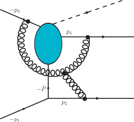
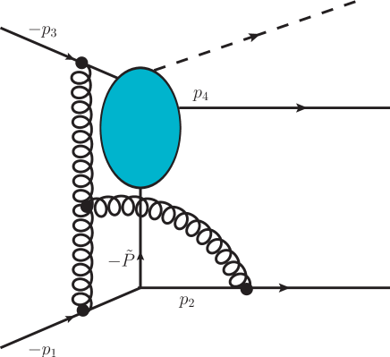
Figure 3: Two-parton SL collinear limit $(p_{i}\simeq z_{i}\widetilde{P},\;i=1,2)$ of two-loop QCD amplitudes with $n=4$ partons and additional colourless external legs (denoted by the dashed line) in parton–parton hard-scattering configurations. Representative colour structure of non-abelian factorization breaking correlations according to (left) Eq. (6.2) and (right) Eq.(6.2).

We present the explicit expression of ${\widetilde{\bf\Delta}}_{C}^{(2)}$ for a generic matrix element with $n=4$ QCD partons (see Fig. 3). We consider only the SL kinematical configurations in which ${\widetilde{\bf\Delta}}_{C}^{(2)}\neq 0$. With no loss of generality, we can limit ourselves to the following kinematical region (the other kinematical regions are obtained by re-labeling the parton momenta):

$$z_{2}<0\;\;,\quad s_{34}<0\;\;,\quad s_{23}<0\;\;,$$

and, using Eq. (146), we have

$${\widetilde{\bf\Delta}}_{C}^{(2)}(\epsilon) = -\;\frac{\alpha_{\mathrm{S}}^{2}(\mu^{2})}{2\pi}\;\left(\frac{-s_{12}}{\mu^{2}}\right)^{\!\!-2\epsilon}\;f_{abc}\;T_{2}^{a}\,T_{3}^{b}\,T_{4}^{c}$$

$$\times \ln\left(-\,\frac{s_{3\widetilde{P}}\;s_{4\widetilde{P}}\,z_{1}z_{2}}{s_{34}\,s_{12}}-i0\right)\;\left[\,-\,\frac{1}{2\,\epsilon^{\,2}}\,+\frac{1}{\epsilon}\;\ln\left(\frac{-z_{2}}{1-z_{2}}\right)\right]$$

$$\simeq \;\frac{\alpha_{\mathrm{S}}^{2}(\mu^{2})}{2\pi}\;\left(\frac{-s_{12}}{\mu^{2}}\right)^{\!\!-2\epsilon}\;f_{abc}\;T_{1}^{a}\,T_{2}^{b}\,T_{3}^{c}$$

$$\times \ln\left(-\,\frac{s_{31}\;s_{42}}{s_{34}\,s_{12}}-i0\right)\;\left[\,-\,\frac{1}{2\,\epsilon^{\,2}}\,+\frac{1}{\epsilon}\;\ln\left(-\frac{z_{2}}{z_{1}}\right)\right]\;\;.$$ (148)

Note that the expressions (6.2) and (6.2) are equivalent in the collinear limit. To obtain Eq. (6.2), we have implemented the collinear approximation $p_{i}\simeq z_{i}\widetilde{P}\;(i=1,2)$, and we have used the $n=4$ equality

$$f_{abc}\;T_{2}^{a}\,T_{3}^{b}\,T_{4}^{c}=\,-\;f_{abc}\;T_{1}^{a}\,T_{2}^{b}\,T_{3}^{c}\;\;,\quad\quad\quad(n=4)\;\;.$$ (149)

This equality derives from charge conservation (i.e., ${{\mbox{\boldmath$T$}}}_{4}=-({{\mbox{\boldmath$T$}}}_{1}+{{\mbox{\boldmath$T$}}}_{2}+{{\mbox{\boldmath$T$}}}_{3})\,$) and from colour algebra, namely, from the general algebraic identity

$$i\,f_{abc}\;T_{i}^{a}\,T_{j}^{b}\,(T_{i}^{c}+T_{j}^{c})=-\,\delta_{ij}\;C_{A}\;{{\mbox{\boldmath$T$}}}_{i}^{2}\;\;.$$ (150)

The factorization breaking correlations depend on the momenta of the non-collinear partons. At the one-loop order (see Eq. (93)), this dependence only involves the sign of the energy of the non-collinear parton (what matter is simply the physical distinction between initial-state and final-state partons). The two-loop operator ${\widetilde{\bf\Delta}}_{C}^{(2)}$ instead depends also on the actual size of the momenta of the non-collinear partons. This dependence appears (see Eq. (146)) through the scale

$$\frac{s_{j\widetilde{P}}\;s_{k\widetilde{P}}}{s_{jk}}\equiv{{\mbox{\boldmath$q$}}}^{2}_{\perp\widetilde{P},jk}\;\;.$$ (151)

We notice that $q^{\mu}_{\perp\widetilde{P},jk}\;$ ($q^{\mu}_{\perp}q_{\perp\mu}=-\,{{\mbox{\boldmath$q$}}}^{2}_{\perp})$ is the component of the momentum $\widetilde{P}^{\mu}$ that is transverse to the direction of the momenta $p_{j}$ and $p_{k}$ in the reference frame where these two momenta are back-to-back. Since in the collinear limit we have $p_{i}\simeq z_{i}\widetilde{P}\;$ ($i=1,2$), the scale (151) can be expressed in terms of the transverse momentum $q^{\mu}_{\perp i,jk}\;$ of one of the collinear partons:

$${{\mbox{\boldmath$q$}}}^{2}_{\perp i,jk}\equiv\frac{s_{ji}\;s_{ki}}{s_{jk}}\simeq z_{i}^{2}\;{{\mbox{\boldmath$q$}}}^{2}_{\perp\widetilde{P},jk}\;\;.$$ (152)

The ‘non-collinear’ scale in Eq. (151) and the ‘collinear’ scale $s_{12}/(z_{1}z_{2})$ are always positive quantities. Thus, we have

$$\ln\left(-\,\frac{s_{j\widetilde{P}}\;s_{k\widetilde{P}}\,z_{1}z_{2}}{s_{jk}\,s_{12}}-i0\right)=\,\ln\left(\,\frac{s_{j\widetilde{P}}\;s_{k\widetilde{P}}\,z_{1}z_{2}}{s_{jk}\,s_{12}}\right)-i\pi\;\;,$$ (153)

where the logarithm on the right-hand side is a real number (with no imaginary part). Inserting Eq. (153) in Eq. (146), we see that ${\widetilde{\bf\Delta}}_{C}^{(2)}$ has a hermitian and an antihermitian part (we recall that at one-loop order the factorization breaking term is purely antihermitian). The hermitian part depends on the non-collinear scale (151). In the antihermitian part, the momenta of the non-collinear partons appear only through the sign of their energies, and we explicitly have

$${\widetilde{\bf\Delta}}_{C}^{(2)}(\epsilon)-\left[{\widetilde{\bf\Delta}}_{C}^{(2)}(\epsilon)\right]^{\dagger} = -\,\frac{i}{2}\;\alpha_{\mathrm{S}}^{2}(\mu^{2})\;\left(\frac{-s_{12}}{\mu^{2}}\right)^{\!\!-2\epsilon}\;f_{abc}\,\sum_{i=1,2}\;\sum_{\begin{subarray}{c}j,k=3\\ j\,\neq\,k\end{subarray}}^{n}\,T_{i}^{a}\,T_{j}^{b}\,T_{k}^{c}\;\Theta(-z_{i})$$

$$\times {\rm sign}(s_{ij})\;\Theta(-s_{jk})\;\left[\,-\,\frac{1}{2\,\epsilon^{\,2}}\,+\frac{1}{\epsilon}\;\ln\left(\frac{-z_{i}}{1-z_{i}}\right)\right]$$

$$= +\,\frac{i}{2}\;\alpha_{\mathrm{S}}^{2}(\mu^{2})\;\left(\frac{-s_{12}}{\mu^{2}}\right)^{\!\!-2\epsilon}\;f_{abc}\,\;\sum_{j=3}^{n}\,T_{1}^{a}\,T_{2}^{b}\,T_{j}^{c}\;{\rm sign}(s_{2j})$$

$$\times \sum_{i=1,2}\;\Theta(-z_{i})\;\left[\,-\,\frac{1}{2\,\epsilon^{\,2}}\,+\frac{1}{\epsilon}\;\ln\left(\frac{-z_{i}}{1-z_{i}}\right)\right]\;\;,$$ (155)

where the equivalence between the expressions (6.2) and (6.2) follows from the conservation of the colour charge (see Eq. (162)). We note that the expression (6.2) involves colour correlations between a non-collinear parton and the two collinear partons. This type of three-parton colour correlations (see, e.g., Fig. 3–right) completes the class of factorization breaking structures that can appear in the two-loop splitting matrix ${{\mbox{\boldmath$Sp$}}}^{(2,R)}$.

We briefly comment on the finite contribution ${\widetilde{{\mbox{\boldmath$Sp$}}}}^{(2)\,{\rm fin.}}$ in Eq. (144). In the TL collinear region, the explicit expression of ${\widetilde{{\mbox{\boldmath$Sp$}}}}^{(2)\,{\rm fin.}}$ at ${\cal O}(\epsilon^{0})$ can be extracted from the direct comparison with the results of Refs. [14, 27]. We have not computed ${\widetilde{{\mbox{\boldmath$Sp$}}}}^{(2)\,{\rm fin.}}$ in the SL collinear region. Its expression contains terms that violate strict collinear factorization. These terms produce all types of colour correlations (including three-parton correlations as in Eq. (6.2)) that contribute to the IR divergent part of ${{\mbox{\boldmath$Sp$}}}^{(2,R)}$.

6.3 Multiparton collinear limit at two-loop order

To our knowledge, no results on the multiparton collinear limit (with $m\geq 3$ collinear partons) of the two-loop QCD amplitudes ${\cal M}^{(2)}$ are available in the literature. To illustrate some main features of the corresponding two-loop splitting matrix ${{\mbox{\boldmath$Sp$}}}^{(2)}$ in the factorization formula (80) (or (86)), we proceed analogously to Sect. 5.3. Considering the renormalized splitting matrix, we introduce the following decomposition in IR divergent and IR finite terms:

$${{\mbox{\boldmath$Sp$}}}^{(2,R)}={{\mbox{\boldmath$Sp$}}}^{(2)\,{\rm div.}}+{{\mbox{\boldmath$Sp$}}}^{(2)\,{\rm fin.}}\;\;.$$ (156)

All the $\epsilon$-pole contributions to ${{\mbox{\boldmath$Sp$}}}^{(2,R)}$ are included in ${{\mbox{\boldmath$Sp$}}}^{(2)\,{\rm div.}}$, which can be written as

$${{\mbox{\boldmath$Sp$}}}^{(2)\,{\rm div.}}={{\mbox{\boldmath$I$}}}^{(1)}_{m\,C}(\epsilon)\;{{\mbox{\boldmath$Sp$}}}^{(1,R)}+{{\mbox{\boldmath$I$}}}^{(2)}_{m\,C}(\epsilon)\;{{\mbox{\boldmath$Sp$}}}^{(0,R)}+{\overline{{\mbox{\boldmath$Sp$}}}}^{(2)\,{\rm div.}}\;\;,$$ (157)

where ${{\mbox{\boldmath$Sp$}}}^{(1,R)}$ is the one-loop splitting matrix, and ${{\mbox{\boldmath$I$}}}^{(1)}_{m\,C}(\epsilon)$ is given in Eq. (98). The new two-loop colour operator ${{\mbox{\boldmath$I$}}}^{(2)}_{m\,C}(\epsilon)$ contains $\epsilon$ poles, and additional IR divergent terms are included in ${\overline{{\mbox{\boldmath$Sp$}}}}^{(2)\,{\rm div.}}$. Note, however, that ${\overline{{\mbox{\boldmath$Sp$}}}}^{(2)\,{\rm div.}}$ is purely non-abelian, it is non-vanishing only in the SL collinear regions, and it contains only single poles (i.e., its IR divergences appear at ${\cal O}(1/\epsilon)$). All the higher-order poles (starting at order ${\cal O}(1/\epsilon^{4})$) are included in the first two terms on the right-hand side of Eq. (157).

The result in Eq. (157) is derived in Appendix B. The derivation is analogous to that of the corresponding result (see Eq. (144)) for the two-parton collinear limit. In the case of the multiparton collinear limit, we do not know the explicit expression of the one-loop splitting matrix ${{\mbox{\boldmath$Sp$}}}^{(1,R)}$ at ${\cal O}(\epsilon^{0})$ in the SL region: this prevent us from computing the explicit expression of ${\overline{{\mbox{\boldmath$Sp$}}}}^{(2)\,{\rm div.}}$ through the method used in Appendix B.

The explicit expression of the colour operator ${{\mbox{\boldmath$I$}}}^{(2)}_{m\,C}$ is

$${{\mbox{\boldmath$I$}}}^{(2)}_{m\,C}(\epsilon) = -\,\frac{1}{2}\left[{{\mbox{\boldmath$I$}}}^{(1)}_{m\,C}(\epsilon)\right]^{2}+\frac{\alpha_{\mathrm{S}}(\mu^{2})}{2\pi}\left\{+\frac{1}{\epsilon}\,b_{0}\left[{{\mbox{\boldmath$I$}}}^{(1)}_{m\,C}(2\epsilon)-{{\mbox{\boldmath$I$}}}^{(1)}_{m\,C}(\epsilon)\right]+K\;{{\mbox{\boldmath$I$}}}^{(1)}_{m\,C}(2\epsilon)\right.$$ (158)

$$+ \,\frac{\alpha_{\mathrm{S}}(\mu^{2})}{2\pi}\left.\,\frac{1}{\epsilon}\;\Bigl{(}\;\sum_{i\,\in C}\,H^{(2)}_{i}\Bigr{.}\Bigl{.}\left.-H^{(2)}_{\widetilde{P}}\right.\Bigr{)}\right\}+{\bf\Delta}_{m\,C}^{(2;\,2)}(\epsilon)\;\;,$$

where

$${\bf\Delta}_{m\,C}^{(2;\,2)}(\epsilon) = \left(\frac{\alpha_{\mathrm{S}}(\mu^{2})}{2\pi}\right)^{2}\left(\,-\,\frac{1}{2\,\epsilon^{2}}\right)\;\pi\;f_{abc}\,\sum_{i\in C}\;\sum_{\begin{subarray}{c}j,k\,\in NC\\ j\,\neq\,k\end{subarray}}\,T_{i}^{a}\,T_{j}^{b}\,T_{k}^{c}\;\Theta(-z_{i})\;{\rm sign}(s_{ij})\;\Theta(-s_{jk})$$ (159)

$$\times \ln\left(-\,\frac{s_{j\widetilde{P}}\;s_{k\widetilde{P}}}{s_{jk}\,\mu^{2}}-i0\right)\;\;.$$

Since the flavour-dependent coefficients $H^{(2)}_{i}$ (the subscript $\widetilde{P}$ in $H^{(2)}_{\widetilde{P}}$ refers to the flavour of the parent collinear parton) are $c$-numbers, the non-trivial colour-charge structure of ${{\mbox{\boldmath$I$}}}^{(2)}_{m\,C}$ is due to ${{\mbox{\boldmath$I$}}}^{(1)}_{m\,C}$ and ${\bf\Delta}_{m\,C}^{(2;\,2)}$. This structure produces violation of strict factorization in the SL collinear regions. In the two-loop splitting matrix ${{\mbox{\boldmath$Sp$}}}^{(2,R)}$, the factorization breaking terms start to contribute at ${\cal O}(1/\epsilon^{3})$ (we recall that ${{\mbox{\boldmath$I$}}}^{(1)}_{m\,C}$ includes the factorization breaking operator ${\bf\Delta}_{m\,C}^{(1)}(\epsilon)$ of Eq. (100)).

The colour-charge operator ${\bf\Delta}_{m\,C}^{(2;\,2)}$ is responsible for some distinctive features of the multiparton collinear limit at two-loop order. This operator is closely analogous to the corresponding operator ${\widetilde{\bf\Delta}}_{C}^{(2)}$ (see Eq. (146)) for the two-parton collinear limit. By direct inspection of Eq. (159), we see that the operator ${\bf\Delta}_{m\,C}^{(2;\,2)}$ produces IR divergences at the level of double poles $1/\epsilon^{2}$, it is non-vanishing only in SL collinear regions, it is definitely non-abelian, and it leads to violation of strict collinear factorization. These factorization breaking terms have the form of three-parton correlations: the colour charge of a collinear parton is correlated to the colour charges of two non-collinear partons (the partons $j$ and $k$) that have energies with opposite sign ($s_{jk}<0$), and the intensity of the correlation is controlled by the transverse-momentum scale ${{\mbox{\boldmath$q$}}}^{2}_{\perp\widetilde{P},jk}$ (see Eq. (151)). Since ${{\mbox{\boldmath$q$}}}^{2}_{\perp\widetilde{P},jk}>0$, the logarithm on the right-hand side of Eq. (159) has a real and an imaginary part (i.e. $\ln(-{{\mbox{\boldmath$q$}}}^{2}_{\perp\widetilde{P},jk}/\mu^{2}-i0)=\ln({{\mbox{\boldmath$q$}}}^{2}_{\perp\widetilde{P},jk}/\mu^{2})-i\pi$) and, correspondingly, the operator ${\bf\Delta}_{m\,C}^{(2;\,2)}$ has a hermitian and an antihermitian part.

Using Eq. (159), the explicit expression of the antihermitian part of ${\bf\Delta}_{m\,C}^{(2;\,2)}$ is

$${\bf\Delta}_{m\,C}^{(2;\,2)}(\epsilon)-\left[\,{\bf\Delta}_{m\,C}^{(2;\,2)}(\epsilon)\right]^{\dagger}\!\!\! = \!\!\!+\,i\;\frac{\alpha_{\mathrm{S}}^{2}(\mu^{2})}{4\,\epsilon^{2}}\;f_{abc}\,\sum_{i\,\in C}\;\sum_{\begin{subarray}{c}j,k\,\in NC\\ j\,\neq\,k\end{subarray}}\,T_{i}^{a}\,T_{j}^{b}\,T_{k}^{c}\;\Theta(-z_{i})\;{\rm sign}(s_{ij})\;\Theta(-s_{jk})$$

$$\simeq \!\!\!-\,i\;\frac{\alpha_{\mathrm{S}}^{2}(\mu^{2})}{4\,\epsilon^{2}}\;f_{abc}\,\sum_{\begin{subarray}{c}i,\ell\,\in C\\ i\,\neq\,\ell\end{subarray}}\;\sum_{j\,\in NC}\,T_{i}^{a}\,T_{\ell}^{b}\,T_{j}^{c}\;\Theta(-z_{i})\;\Theta(-s_{i\ell})\;{\rm sign}(s_{j\widetilde{P}})\;.$$

The expressions (6.3) and (6.3) are equivalent in the collinear limit (see Eq. (162) and the accompanying comments in the final part of this subsection). In particular, Eq. (6.3) shows that the antihermitian part of ${\bf\Delta}_{m\,C}^{(2;\,2)}$ can be expressed in terms of three-parton correlations that involve a non-collinear parton and two collinear partons (the partons $i$ and $\ell$) that have energies with opposite sign ($s_{i\ell}<0$).

We add some brief comments on the two-loop contributions ${\overline{{\mbox{\boldmath$Sp$}}}}^{(2)\,{\rm div.}}$ (see Eq. (157)) and ${{\mbox{\boldmath$Sp$}}}^{(2)\,{\rm fin.}}$ (see Eq. (156)). The term ${\overline{{\mbox{\boldmath$Sp$}}}}^{(2)\,{\rm div.}}$, which is proportional to the single pole $1/\epsilon$, is non-vanishing only in SL collinear regions and (analogously to ${\bf\Delta}_{m\,C}^{(2;\,2)}$) it involves non-abelian factorization breaking correlations between a collinear parton and two non-collinear partons (see Eq. (233)). The IR finite term ${{\mbox{\boldmath$Sp$}}}^{(2)\,{\rm fin.}}$ is non-vanishing in both the TL and SL collinear regions. In the SL collinear limit, ${{\mbox{\boldmath$Sp$}}}^{(2)\,{\rm fin.}}$ receives factorization breaking contributions from all types of colour correlations that appear in ${{\mbox{\boldmath$Sp$}}}^{(2)\,{\rm div.}}$. In particular, ${{\mbox{\boldmath$Sp$}}}^{(2)\,{\rm fin.}}$ also includes non-abelian correlations between a non-collinear parton and two collinear partons (see, e.g., Eq. (6.3)).

Factorization breaking terms that correlate the colour matrices of three partons can be related by using the following identity:

$$f_{abc}\,\sum_{i\in C}\;\sum_{\begin{subarray}{c}j,k\,\in NC\\ j\,\neq\,k\end{subarray}}\,T_{i}^{a}\,T_{j}^{b}\,T_{k}^{c}\;\,{\rm sign}(s_{ij})\;\Theta(-s_{jk})\;h_{i}=f_{abc}\,\sum_{\begin{subarray}{c}i,\,\ell\,\in C\\ i\,\neq\,\ell\end{subarray}}\;\sum_{j\in NC}\,T_{i}^{a}\,T_{\ell}^{b}\,T_{j}^{c}\;\,{\rm sign}(s_{ij})\;h_{i}\;\;,$$ (162)

where $h_{i}$ is an arbitrary $c$-number function that depends on the collinear parton $i$. The identity (162) relates terms that involve one collinear parton and two non-collinear partons to terms that involve two collinear partons and one non-collinear parton. Note that this relation requires that the kinematical function $h_{i}$ is independent of the non-collinear partons (e.g., of the momenta of the non-collinear partons). If the function $h_{i}$ is simply $h_{i}=\Theta(-z_{i})$, we can implement the collinear limit $p_{i}\simeq z_{i}\widetilde{P}$ and we can rewrite the right-hand side of Eq. (162) as follows:

$$f_{abc}\sum_{\begin{subarray}{c}i,\,\ell\,\in C\\ i\,\neq\,\ell\end{subarray}}\sum_{j\in NC}T_{i}^{a}T_{\ell}^{b}T_{j}^{c}\,{\rm sign}(s_{ij})\,\Theta(-z_{i})\simeq-f_{abc}\sum_{\begin{subarray}{c}i,\,\ell\,\in C\\ i\,\neq\,\ell\end{subarray}}\sum_{j\in NC}T_{i}^{a}T_{\ell}^{b}T_{j}^{c}\,{\rm sign}(s_{j\widetilde{P}})\,\Theta(-z_{i})\,\Theta(-s_{i\ell})\,.$$ (163)

The proof of Eq. (162) (which follows from colour conservation) and the derivation of the collinear relation (163) are presented in Appendix B (see Eqs. (245)–(249)). The expression (6.3) is obtained from (6.3) by simply using Eqs. (162) and (163). The expression (6.2) is obtained from (6.2) by directly using Eq. (162) (note that ${\rm sign}(s_{1j})=-\,{\rm sign}(s_{2j})$ in the SL collinear region, since $s_{12}<0$).

7 Squared amplitudes and cross sections

The perturbative QCD computation of cross sections (and related physical observables) requires the evaluation of the square of the matrix element ${\cal M}(p_{1},p_{2},\dots,p_{n})$ and its integration over the phase space of the final-state partons. In this section we consider the collinear limit of squared amplitudes. In particular, we are interested in the implications of violation of strict collinear factorization at the level of squared amplitudes and, possibly, of cross sections.

7.1 The collinear behaviour of squared amplitudes

We consider the squared matrix element, $|{\cal M}|^{2}$, summed over the colours and spins of the external QCD partons (see Eq. (7)):

$$|{\cal M}(p_{1},p_{2},\dots)|^{2}\equiv\sum_{\{c_{i}\}}\,\sum_{\{s_{i}\}}\;\Bigl{[}\,{\cal M}^{c_{1},c_{2},\dots;s_{1},s_{2},\dots}(p_{1},p_{2},\dots)\,\Bigr{]}^{\dagger}\;{\cal M}^{c_{1},c_{2},\dots;s_{1},s_{2},\dots}(p_{1},p_{2},\dots)\,\;\;.$$ (164)

Using the notation in colour+spin space (see Eq. (8)), $|{\cal M}|^{2}$ can be written as

$$|{\cal M}(p_{1},p_{2},\dots,p_{n})|^{2}=\langle\,{\cal M}(p_{1},p_{2},\dots,p_{n})\,|\,{\cal M}(p_{1},p_{2},\dots,p_{n})\,\rangle\;\;.$$ (165)

The all-order singular behaviour of $|{\cal M}|^{2}$, in a generic kinematical configuration of $m$ collinear partons with momenta $\{p_{1},\dots,p_{m}\}$, is obtained by squaring the generalized factorization formula in Eq. (78). We have

$$|{\cal M}|^{2}\;\simeq\langle\,{\overline{\cal M}}\,|\,\;{\bf P}(p_{1},\dots,p_{m};{\widetilde{P}};p_{m+1},\dots,p_{n})\;\;|{{\overline{\cal M}}}\rangle\;\;,$$ (166)

where the matrix ${\bf P}$ is the square of the all-order splitting matrix $Sp$ :

$${\cal{\bf P}}\equiv\left[\,{{\mbox{\boldmath$Sp$}}}\,\right]^{\dagger}\,{{\mbox{\boldmath$Sp$}}}\;\;.$$ (167)

The loop expansion of the squared splitting matrix ${\bf P}$ is

$${\bf P}={\bf P}^{(0,R)}+{\bf P}^{(1,R)}+{\bf P}^{(2,R)}+\dots\;\;,$$ (168)

where ${\bf P}^{(k,R)}$ (with $k=0,1,2,\dots$) are the renormalized perturbative contributions. Inserting Eq. (83) in Eq. (167), we obtain the expression of ${\bf P}^{(k,R)}$ in terms of the perturbative contributions to $Sp$ :

$${\bf P}^{(0,R)}=\left(\,{{\mbox{\boldmath$Sp$}}}^{(0,R)}\,\right)^{\dagger}\,{{\mbox{\boldmath$Sp$}}}^{(0,R)}\;\;,$$ (169)

$${\bf P}^{(1,R)}=\left(\,{{\mbox{\boldmath$Sp$}}}^{(0,R)}\,\right)^{\dagger}\,{{\mbox{\boldmath$Sp$}}}^{(1,R)}\;+\;{\rm h.c.}\;\;,$$ (170)

$${\bf P}^{(2,R)}=\left(\,{{\mbox{\boldmath$Sp$}}}^{(1,R)}\,\right)^{\dagger}\,{{\mbox{\boldmath$Sp$}}}^{(1,R)}\,+\left[\left(\,{{\mbox{\boldmath$Sp$}}}^{(0,R)}\,\right)^{\dagger}\,{{\mbox{\boldmath$Sp$}}}^{(2,R)}+\;{\rm h.c.}\right]\;\;,$$ (171)

where the abbreviation ‘h.c.’ means hermitian conjugate.

The perturbative (loop) expansion of the all-order factorization formula (166) is obtained by using Eqs. (82) and (168). Considering the expansion up to the two-loop level, we have

$$|\,{\cal M}^{(0,R)}\,|^{2}\simeq\langle\,{\overline{\cal M}}^{(0,R)}\,|\,\;{\bf P}^{(0,R)}\;\;|{{\overline{\cal M}}^{(0,R)}}\rangle\;\;,$$ (172)

$$\langle\,{\cal M}^{(0,R)}\,|{{\cal M}^{(1,R)}}\rangle+\;{\rm c.c.}\;\simeq\left[\langle\,{\overline{\cal M}}^{(0,R)}\,|\,\;{\bf P}^{(0,R)}\;|{{\overline{\cal M}}^{(1,R)}}\rangle+\;{\rm c.c.}\;\right]+\langle\,{\overline{\cal M}}^{(0,R)}\,|\,{\bf P}^{(1,R)}\;|{{\overline{\cal M}}^{(0,R)}}\rangle\;,$$ (173)

$$|\,{\cal M}^{(1,R)}\,|^{2}\!\!\!\!\!\!\!\! +\Bigl{[}\;\langle\,{\cal M}^{(0,R)}\,|{{\cal M}^{(2,R)}}\rangle+\;{\rm c.c.}\;\Bigr{]}\simeq\langle\,{\overline{\cal M}}^{(1,R)}\,|\,\;{\bf P}^{(0,R)}\;|{{\overline{\cal M}}^{(1,R)}}\rangle$$ (174)

$$+\left[\langle\,{\overline{\cal M}}^{(0,R)}\,|\,\;{\bf P}^{(0,R)}\;|{{\overline{\cal M}}^{(2,R)}}\rangle+\;{\rm c.c.}\;\right]+\left[\langle\,{\overline{\cal M}}^{(0,R)}\,|\,\;{\bf P}^{(1,R)}\;|{{\overline{\cal M}}^{(1,R)}}\rangle+\;{\rm c.c.}\;\right]$$

$$+\;\langle\,{\overline{\cal M}}^{(0,R)}\,|\,{\bf P}^{(2,R)}\;|{{\overline{\cal M}}^{(0,R)}}\rangle\;\;,$$

where the abbreviation ‘c.c.’ means complex conjugate. The tree-level factorization formula (172) depends on ${\bf P}^{(0,R)}$. The one-loop factorization formula (173) also depends on ${\bf P}^{(1,R)}$, whereas ${\bf P}^{(2,R)}$ enters the two-loop factorization formula (174). The expressions in Eqs. (172), (173) and (174) directly correspond to the terms that contribute to the order-by-order perturbative calculation of cross sections.

The kernel ${\bf P}$ on the right-hand side of the generalized factorization formula (166) is a matrix in colour+spin space. The matrix acts on the vector space of the reduced matrix element ${{\overline{\cal M}}\,({\widetilde{P}},p_{m+1},\dots,p_{n})}$. The dependence of ${\bf P}$ on the spin and colour indices can be denoted in the following explicit form:

$$\langle{c^{\prime},c^{\prime}_{m+1},\dots,c^{\prime}_{n}}|\left[\,{\bf P}(p_{1},\dots,p_{m};{\widetilde{P}};p_{m+1},\dots,p_{n})\,\right]_{s^{\prime}s}|{c,c_{m+1},\dots,c_{n}}\rangle\;\;,$$ (175)

where $c_{m+1},\dots,c_{n}$ are the colour indices of the non-collinear partons (with momenta $p_{m+1},\dots,p_{n}$) in $|{{\overline{\cal M}}}\rangle$, whereas $c$ and $s$ are the colour and spin indices of the parent collinear parton (with momentum $\widetilde{P}$) in $|{{\overline{\cal M}}}\rangle$ (the indices $c^{\prime}_{m+1},\dots,c^{\prime}_{n},c^{\prime}$ and $s^{\prime}$ refer to the vector space of the complex conjugate matrix element $\langle{{\overline{\cal M}}}|\,$). The matrix structure of Eq. (175) follows from Eq. (167) and from the matrix structure of the splitting matrix $Sp$. We briefly comment on the dependence of Eq. (175) on the spin and colour indices, in turn.

According to the generalized factorization formula (78), the splitting matrix $Sp$ is independent of the spin of the non-collinear partons: indeed, $Sp$ only depends on the spin indices of the collinear partons and of the parent collinear parton. Since the right-hand side of Eq. (167) (or, equivalently, the left-hand side of Eq. (166)) involves the (implicit) sum over the spins of the collinear partons, the squared splitting matrix ${\bf P}$ can only depend on the spin indices, $s$ and $s^{\prime}$, of the parent collinear parton (as explicitly denoted in Eq. (175)). The parent collinear parton can be either a quark (antiquark) or a gluon, and we recall (see, e.g., Ref. [11]) that the spin structure of $\left[\,{\bf P}\,\right]_{s^{\prime}s}$ is different in these two cases. Fermion helicity is conserved by QCD radiation from massless quarks (antiquarks). Therefore, if the parent collinear parton is a fermion (quark or antiquark), we can consider the helicity basis in spin space and the squared splitting matrix ${\bf P}$ turns out to be diagonal in this basis: actually, due to parity invariance, we simply have $\left[\,{\bf P}\,\right]_{s^{\prime}s}\propto\delta_{s^{\prime}s}$. An analogous reasoning cannot be applied if the parent collinear parton is a gluon. In the gluon case, $\left[\,{\bf P}\,\right]_{s^{\prime}s}$ has a non-trivial dependence on the gluon spin indices $s$ and ${s^{\prime}}$. This dependence has to carefully be taken into account (see, e.g., Refs. [35] and [51, 52]) to achieve the cancellation of IR, soft and collinear divergences in calculations of cross sections. Moreover (see Refs. [53, 54]), the dependence of $\left[\,{\bf P}\,\right]_{s^{\prime}s}$ on the gluon spin indices can lead to physically-observable and logarithmically-enhanced effects in specific kinematical configurations.

The colours of the collinear partons are (implicitly) summed on the right-hand side of Eq. (167) (or, equivalently, on the left-hand side of Eq. (166)) and thus, in general, the squared splitting matrix ${\bf P}$ depends on the colour indices of the parent collinear parton and of the non-collinear partons (as explicitly denoted in Eq. (175)). In the TL collinear region, strict factorization is valid: since $Sp$ is independent of the colours of the non-collinear partons, the squared matrix ${\bf P}$ is also independent of them and it can only depend on the colours, $c$ and $c^{\prime}$, of the parent collinear parton. Owing to colour conservation, this residual colour dependence is, however, trivial: it is diagonal and simply proportional to $\delta_{c^{\prime}c}$. In summary, considering the TL collinear region, ${\bf P}$ is proportional to the unit matrix in colour space, and the matrix structure in Eq. (175) simplifies as follows:

$$\left[\,{\cal P}(p_{1},\dots,p_{m};{\widetilde{P}})\,\right]_{s^{\prime}s}\;\delta_{c^{\prime}c}\;\delta_{c^{\prime}_{m+1}c_{m+1}}\;\dots\;\delta_{c^{\prime}_{n}c_{n}}\;\;,\;\;\quad({\rm TL\,\;coll.\,\;lim.})\;\;,$$ (176)

where the matrix ${\cal P}_{s^{\prime}s}$ only depends on the spin indices of the parent collinear parton. The strictly factorized version of Eq. (166) in the TL collinear region is

$$|{\cal M}|^{2}\;\simeq\sum_{s,s^{\prime}}\;\left[\,{\cal P}(p_{1},\dots,p_{m};{\widetilde{P}})\,\right]_{s^{\prime}s}\;\langle\,{\overline{\cal M}}\,|{s^{\prime}}\rangle\;\langle\,s\,|{{\overline{\cal M}}}\rangle\;\;,\;\;\quad({\rm TL\,\;coll.\,\;lim.})\;.$$ (177)

In the SL collinear region, the simplified structure of Eqs. (176) and (177) is valid only at the tree level (i.e. it applies only to ${\bf P}^{(0,R)}$ in Eqs. (169) and (172)). Beyond the tree level, the SL collinear limit violates strict factorization, and the perturbative contributions ${\bf P}^{(1,R)}$ and ${\bf P}^{(2,R)}$ in Eqs. (173) and (174) depend on the non-collinear partons (as generically denoted in Eq. (175)). In the following subsections, we present explicit expressions for the one-loop and two-loop collinear matrices, ${\bf P}^{(1,R)}$ and ${\bf P}^{(2,R)}$, and we discuss the structure of the terms that produce violation of strict collinear factorization at the squared amplitude level in the SL collinear region.

7.2 Two-parton collinear limit of squared amplitudes

We consider the two-parton collinear splitting $A\rightarrow A_{1}A_{2}$ in a generic (TL or SL) kinematical region. The corresponding tree-level collinear matrix ${\bf P}^{(0,R)}={\bf P}^{(0,R)}(p_{1},p_{2};\widetilde{P})$ is strictly factorized. It can be computed (see Eq. (169)) by squaring the splitting matrices in Eqs. (12)–(2). The four-dimensional expression for ${\bf P}^{(0,R)}$ is well known [15], and the explicit $d$-dimensional expressions in various variants of dimensional regularization are given in Ref. [45].

The one-loop collinear matrix ${\bf P}^{(1,R)}$ is computed by inserting the splitting matrix ${{\mbox{\boldmath$Sp$}}}^{(1,R)}$ of Eq. (92) in Eq. (170). We straightforwardly obtain the result

$${\bf P}^{(1,R)}={\widetilde{I}}_{P}^{(1)}(\epsilon)\;{\bf P}^{(0,R)}+\left[\left(\,{{\mbox{\boldmath$Sp$}}}^{(0,R)}\,\right)^{\dagger}\,{{\mbox{\boldmath$Sp$}}}^{(1,R)}_{H}+\;{\rm h.c.}\;\right]\;\;,$$ (178)

where the IR divergent factor ${\widetilde{I}}_{P}^{(1)}(\epsilon)$ is

$${\widetilde{I}}_{P}^{(1)}(\epsilon)={\widetilde{{\mbox{\boldmath$I$}}}}_{C}^{(1)}(\epsilon)+\;{\rm h.c.}\;\;.$$ (179)

Inserting the explicit expression of the colour operator ${\widetilde{{\mbox{\boldmath$I$}}}}_{C}^{(1)}$ (see Eq. (93)) in Eq. (179), the factor ${\widetilde{I}}_{P}^{(1)}$ turns out to be a $c$-number (more precisely, ${\widetilde{I}}_{P}^{(1)}$ is simply proportional to the unit matrix in colour space). We explicitly obtain the following expression:

$${\widetilde{I}}_{P}^{(1)}(\epsilon) = \frac{\alpha_{\mathrm{S}}(\mu^{2})}{2\pi}\;\frac{1}{2}\;\,{\widetilde{c}}_{\Gamma}\;\left[\left(\frac{-s_{12}-i0}{\mu^{2}}\right)^{-\epsilon}+\;{\rm c.c.}\;\right]$$ (180)

$$\times \left\{\;\frac{1}{\epsilon^{2}}\;\Bigl{(}C_{12}-C_{1}-C_{2}\Bigr{)}+\frac{1}{\epsilon}\;\Bigl{(}\gamma_{12}-\gamma_{1}-\gamma_{2}\Bigr{)}\right.$$

$$- \left.\;\frac{1}{\epsilon}\,\left[\Bigl{(}C_{12}+C_{1}-C_{2}\Bigr{)}\;f_{R}(\epsilon;z_{1})+\Bigl{(}C_{12}+C_{2}-C_{1}\Bigr{)}\;f_{R}(\epsilon;z_{2})\;\right]\;\right\}\;\;.$$

An important conclusion to be drawn from the result in Eq. (178) is that ${\bf P}^{(1,R)}$ is strictly factorized, despite the fact that the corresponding one-loop splitting matrix ${{\mbox{\boldmath$Sp$}}}^{(1,R)}$ violates strict collinear factorization in the SL collinear region. The contribution ${{\mbox{\boldmath$Sp$}}}_{H}^{(1,R)}$ in Eq. (92) is strictly factorized, and the factorization breaking terms of ${{\mbox{\boldmath$Sp$}}}^{(1,R)}$ are entirely embodied in ${\widetilde{{\mbox{\boldmath$I$}}}}_{C}^{(1)}$. However, these terms are antihermitian and, therefore, they cancel (see Eq. (179)) in the computation of the squared splitting matrix ${\bf P}^{(1,R)}$. The absence of factorization breaking terms in ${\bf P}^{(1,R)}$ implies that, in the specific case of the two-parton collinear limit, the factorization structure of Eq. (177) is valid up to the one-loop level (this factorization structure can be implemented in the one-loop formula (173)).

The result in Eqs. (178) and (180) also suggests a practical recipe to compute ${\bf P}^{(1,R)}$ (in both the TL and SL regions) by-passing the violation of strict collinear factorization at the amplitude level. The recipe is: consider the expression of ${{\mbox{\boldmath$Sp$}}}^{(1,R)}$ in the TL collinear region (this expression is strictly factorized, but it depends on the function $f(\epsilon;x)$ that is ill-defined in the SL collinear region), replace $f(\epsilon;x)$ with its (well-defined) real part $f_{R}(\epsilon;x)$ (see Eq. (54)), and use the corresponding expression of ${{\mbox{\boldmath$Sp$}}}^{(1,R)}$ to compute ${\bf P}^{(1,R)}$. This practical recipe, which gives the correct result in Eq. (178), coincides with the ‘effective prescription’ proposed in Refs. [27] (see Sect. 7.4 therein) to perform the analytic continuation of ${\bf P}^{(1,R)}$ from the TL into the SL collinear regions. An extension of this practical recipe from one-loop to two-loop level is not feasible. Indeed, as shown below, the two-loop matrix ${\bf P}^{(2,R)}$ is not strictly factorized in the SL collinear region.

The one-loop SL prescription (recipe) that we have just illustrated was used in practice in the actual NNLO computation of Ref. [55]. This prescription is also consistent with the one-loop calculation of the initial-initial three-parton antenna functions (see Eq. (3.19) in Ref. [56]). Incidentally, we note that the initial-initial antenna functions derived in Ref. [56] are based on explicit one-loop computations of specific squared amplitudes with $n=3$ QCD partons (e.g., the squared amplitude of the DY subprocess $q{\bar{q}}\rightarrow\gamma^{*}g$). Therefore, the universality (process independence) of those initial-initial three-parton antenna functions is eventually a consequence of the strict factorization of the one-loop collinear matrix ${\bf P}^{(1,R)}$ for the SL collinear limit of $m=2$ partons.

The right-hand side of the two-loop collinear relation (174) has four contributions. The first three contributions depend on ${\bf P}^{(0,R)}$ and ${\bf P}^{(1,R)}$ (which are strictly factorized), and the last contribution depends on ${\bf P}^{(2,R)}$. The two-loop collinear matrix ${\bf P}^{(2,R)}$ can be computed by inserting Eqs. (92), (144) and (145) in Eq. (171). Performing some algebraic operations, we obtain

$${\bf P}^{(2,R)} = {\widetilde{I}}_{P}^{(1)}(\epsilon)\;{\bf P}^{(1,R)}+{\widetilde{I}}_{P}^{(2)}(\epsilon)\;{\bf P}^{(0,R)}+\left({{\mbox{\boldmath$Sp$}}}_{H}^{(1,R)}\,\right)^{\dagger}\,{{\mbox{\boldmath$Sp$}}}_{H}^{(1,R)}$$ (181)

$$+ \left({{\mbox{\boldmath$Sp$}}}^{(0,R)}\,\right)^{\dagger}\;{\widetilde{\bf\Delta}}_{P}^{(2)}(\epsilon)\;{{\mbox{\boldmath$Sp$}}}^{(0,R)}+\left[\left({{\mbox{\boldmath$Sp$}}}^{(0,R)}\,\right)^{\dagger}\,{\widetilde{{\mbox{\boldmath$Sp$}}}}^{(2)\,{\rm fin.}}+\;{\rm h.c.}\;\right]\;\;,$$

where ${\widetilde{I}}_{P}^{(1)}(\epsilon)$ is given in Eq. (180), and the two-loop IR divergent factor ${\widetilde{I}}_{P}^{(2)}(\epsilon)$ is

$${\widetilde{I}}_{P}^{(2)}(\epsilon) = -\,\frac{1}{2}\left[{\widetilde{I}}_{P}^{(1)}(\epsilon)\right]^{2}+\frac{\alpha_{\mathrm{S}}(\mu^{2})}{2\pi}\left\{\,\frac{1}{\epsilon}\,b_{0}\left[\,{\widetilde{I}}_{P}^{(1)}(2\epsilon)-{\widetilde{I}}_{P}^{(1)}(\epsilon)\right]+K\;{\widetilde{I}}_{P}^{(1)}(2\epsilon)\right.$$ (182)

$$+ \,\frac{\alpha_{\mathrm{S}}(\mu^{2})}{2\pi}\left[\left(\frac{-s_{12}-i0}{\mu^{2}}\right)^{\!-2\epsilon}+\;{\rm c.c.}\;\right]\left.\,\frac{1}{\epsilon}\;\Bigl{(}\,H^{(2)}_{1}+H^{(2)}_{2}\Bigr{.}\Bigl{.}\left.-H^{(2)}_{12}\right.\Bigr{)}\right\}\;\;.$$

Since ${\widetilde{I}}_{P}^{(2)}(\epsilon)$ is a $c$-number, the first three terms on the right-hand side of Eq. (181) are strictly factorized. The last two terms, instead, lead to violation of strict collinear factorization. The last term, which depends on ${\widetilde{{\mbox{\boldmath$Sp$}}}}^{(2)\,{\rm fin.}}$, is IR finite. The operator ${\widetilde{\bf\Delta}}_{P}^{(2)}(\epsilon)$ is IR divergent and it originates from the colour operator ${\widetilde{\bf\Delta}}_{C}^{(2)}$ on the right-hand side of Eq. (145); we have

$${\widetilde{\bf\Delta}}_{P}^{(2)}(\epsilon)={\widetilde{\bf\Delta}}_{C}^{(2)}(\epsilon)+\;{\rm h.c.}\;\;.$$ (183)

Inserting the explicit expression of ${\widetilde{\bf\Delta}}_{C}^{(2)}(\epsilon)$ (see Eq. (146)) in Eq. (183), we obtain

$${\widetilde{\bf\Delta}}_{P}^{(2)}(\epsilon) = \left(\frac{\alpha_{\mathrm{S}}(\mu^{2})}{2\pi}\right)^{2}\;\left(\frac{-s_{12}}{\mu^{2}}\right)^{\!\!-2\epsilon}2\;\pi\;f_{abc}\,\sum_{i=1,2}\;\sum_{\begin{subarray}{c}j,k=3\\ j\,\neq\,k\end{subarray}}^{n}\,T_{i}^{a}\,T_{j}^{b}\,T_{k}^{c}\;\Theta(-z_{i})\;{\rm sign}(s_{ij})\;\Theta(-s_{jk})$$ (184)

$$\times \ln\left(\,\frac{s_{j\widetilde{P}}\;s_{k\widetilde{P}}\,z_{1}z_{2}}{s_{jk}\,s_{12}}\right)\;\left[\,-\,\frac{1}{2\,\epsilon^{\,2}}\,+\frac{1}{\epsilon}\;\ln\left(\frac{-z_{i}}{1-z_{i}}\right)\right]\;\;.$$

Note that the argument of the logarithm in Eq. (184) can be replaced by using the approximation

$$\frac{s_{j\widetilde{P}}\;s_{k\widetilde{P}}\,z_{1}z_{2}}{s_{jk}\,s_{12}}\simeq\frac{s_{j1}\;s_{k2}}{s_{jk}\,s_{12}}\simeq\frac{s_{j2}\;s_{k1}}{s_{jk}\,s_{12}}\;\;,$$ (185)

which is valid in the collinear limit ($p_{i}\simeq z_{i}\widetilde{P},$ with $i=1,2$).

The expression (144) for ${{\mbox{\boldmath$Sp$}}}^{(2,R)}$ includes several terms that violate strict collinear factorization, and most of them cancel in the computation of ${\bf P}^{(2,R)}$. Many factorization breaking terms of ${{\mbox{\boldmath$Sp$}}}^{(2,R)}$ have a one-loop origin and are included in the operator ${\widetilde{{\mbox{\boldmath$I$}}}}_{C}^{(1)}$. These one-loop terms do not appear in ${\bf P}^{(2,R)}$: their cancellation is due to the iterative dependence of ${{\mbox{\boldmath$Sp$}}}^{(2,R)}$ on ${{\mbox{\boldmath$Sp$}}}^{(1,R)}$ and ${\widetilde{{\mbox{\boldmath$I$}}}}_{C}^{(1)}$, and to the fact that the factorization breaking part of ${\widetilde{{\mbox{\boldmath$I$}}}}_{C}^{(1)}$ is antihermitian. The two-loop factorization breaking operator ${\widetilde{\bf\Delta}}_{C}^{(2)}$ has instead a hermitian component that leads to the operator ${\widetilde{\bf\Delta}}_{P}^{(2)}$ (see Eqs. (183) and (184)) and, thus, to ensuing factorization breaking terms in ${\bf P}^{(2,R)}$. Additional (though IR finite) factorization breaking contributions to ${\bf P}^{(2,R)}$ are produced by ${\widetilde{{\mbox{\boldmath$Sp$}}}}^{(2)\,{\rm fin.}}$.

The IR divergent colour operator ${\widetilde{\bf\Delta}}_{P}^{(2)}(\epsilon)$ is non-abelian and it is non-vanishing only in the SL collinear region. The main features of ${\widetilde{\bf\Delta}}_{P}^{(2)}$ are similar to those of the operator ${\widetilde{\bf\Delta}}_{C}^{(2)}$ (see the related discussion in Sect. 6.2). In particular, ${\widetilde{\bf\Delta}}_{C}^{(2)}$ and, hence, ${\widetilde{\bf\Delta}}_{P}^{(2)}$ vanish in the case of the SL collinear limit of the amplitudes that are involved in lepton–hadron DIS. Moreover, it is important to note (as discussed below) that ${\widetilde{\bf\Delta}}_{P}^{(2)}$ gives a vanishing contribution to ${\bf P}^{(2,R)}$ in the case of scattering amplitudes ${\cal M}(p_{1},\dots,p_{n})$ with $n\leq 4$ QCD partons (and an arbitrary number of colourless external legs). Therefore, to detect the effect of ${\widetilde{\bf\Delta}}_{P}^{(2)}$ at the squared amplitude level, we have to consider the SL collinear limit of amplitudes with $n\geq 5$ QCD partons.

The explicit expression of ${\widetilde{\bf\Delta}}_{C}^{(2)}$ for a generic matrix element with $n=4$ QCD partons (if $n=3$, ${\widetilde{\bf\Delta}}_{C}^{(2)}$ vanishes trivially, as noticed in Sect. 6.2) is given in Eq. (6.2). Independently of the specific kinematical configuration, colour conservation implies that ${\widetilde{\bf\Delta}}_{C}^{(2)}$ and, hence, ${\widetilde{\bf\Delta}}_{P}^{(2)}$ are proportional to a single colour charge operator; we have

$${\widetilde{\bf\Delta}}_{P}^{(2)}(\epsilon)\propto\;f_{abc}\;T_{1}^{a}\,T_{2}^{b}\,T_{3}^{c}\;\;,\quad\quad(n=4)\;\;.$$ (186)

We note that, in the case of the two-parton collinear limit, the tree-level splitting matrix ${{\mbox{\boldmath$Sp$}}}^{(0,R)}$ fulfils the following colour charge relation:

$$\left({{\mbox{\boldmath$Sp$}}}^{(0,R)}(p_{1},p_{2};\widetilde{P})\right)^{\dagger}\;f_{abc}\,T_{1}^{a}\,T_{2}^{b}\,\;{{\mbox{\boldmath$Sp$}}}^{(0,R)}(p_{1},p_{2};\widetilde{P})=0$$ (187)

Therefore, Eqs. (186) and (187) imply:

$$\left({{\mbox{\boldmath$Sp$}}}^{(0,R)}\right)^{\dagger}\;{\widetilde{\bf\Delta}}_{P}^{(2)}\;\;{{\mbox{\boldmath$Sp$}}}^{(0,R)}=0\;\;,\quad\quad(n=4)\;\;,$$ (188)

and, hence, ${\widetilde{\bf\Delta}}_{P}^{(2)}$ does not contribute to ${\bf P}^{(2,R)}$ (see Eq. (181)) if $n=4$.

The relation (187) follows from colour conservation. The proof is very simple. Using Eq. (41) and the fact that the Casimir factor $C_{12}$ is a real $c$-number ($C_{12}^{*}=C_{12}$), we obtain

$$\left({{\mbox{\boldmath$Sp$}}}^{(0,R)}\right)^{\dagger}\;\left[\,T_{1}^{c}\,,({{\mbox{\boldmath$T$}}}_{1}+{{\mbox{\boldmath$T$}}}_{2})^{2}\,\right]\;\;{{\mbox{\boldmath$Sp$}}}^{(0,R)}=\left({{\mbox{\boldmath$Sp$}}}^{(0,R)}\right)^{\dagger}\;\left(\,T_{1}^{c}\,C_{12}-C_{12}\,T_{1}^{c}\,\right)\;{{\mbox{\boldmath$Sp$}}}^{(0,R)}=0\;\;.$$ (189)

Moreover, using elementary colour algebra, the commutator in Eq. (189) gives

$$i\,\left[\,T_{1}^{c}\,,({{\mbox{\boldmath$T$}}}_{1}+{{\mbox{\boldmath$T$}}}_{2})^{2}\,\right]=2\,f_{abc}\;T_{1}^{a}\,T_{2}^{b}\;\;.$$ (190)

Inserting Eq. (190) in Eq. (189), we get the result in Eq. (187).

The operator ${\widetilde{\bf\Delta}}_{P}^{(2)}$ contributes to the SL collinear limit of the squared amplitudes (with $n\geq 5$ partons) that are involved in hadron–hadron hard-scattering processes. We explicitly consider a typical example with $n=5$ partons: the process ‘parton + parton $\rightarrow$ 3 partons’ (see Fig. 4) or, more generally, ‘parton + parton $\rightarrow X+$ 3 partons’ ($X$ denotes non-QCD particles, e.g. a vector boson), where one of the final-state partons is collinear to one of the initial-state partons. We specify the parton momenta as follows: the two initial-state partons have momenta $-p_{1}$ and $-p_{3}$ (i.e., the ‘energies’ $p_{1}^{0}$ and $p_{3}^{0}$ are negative), and the three final-state partons have momenta $p_{2},p_{4}$ and $p_{5}$ (i.e., $p_{2}^{0},p_{4}^{0}$ and $p_{5}^{0}$ are positive). Since $z_{2}<0<z_{1}$ and $s_{45}>0$, there are only two different colour operators that contribute to the expression (184) of ${\widetilde{\bf\Delta}}_{P}^{(2)}$: these operators are $f_{abc}\;T_{2}^{a}\,T_{3}^{b}\,T_{4}^{c}$ and $f_{abc}\;T_{2}^{a}\,T_{3}^{b}\,T_{5}^{c}$. Using colour conservation (i.e., ${{\mbox{\boldmath$T$}}}_{5}=-({{\mbox{\boldmath$T$}}}_{1}+{{\mbox{\boldmath$T$}}}_{2}+{{\mbox{\boldmath$T$}}}_{3}+{{\mbox{\boldmath$T$}}}_{4})$) and the identity (150), we obtain

$$f_{abc}\;T_{2}^{a}\,T_{3}^{b}\,T_{5}^{c}=-f_{abc}\;T_{2}^{a}\,T_{3}^{b}\,T_{4}^{c}-f_{abc}\;T_{2}^{a}\,T_{3}^{b}\,T_{1}^{c}\;\;,\quad\quad(n=5)\;\;,$$ (191)

and we can write ${\widetilde{\bf\Delta}}_{P}^{(2)}$ in terms of the colour operators $f_{abc}\;T_{2}^{a}\,T_{3}^{b}\,T_{4}^{c}$ and $f_{abc}\;T_{1}^{a}\,T_{2}^{b}\,T_{3}^{c}$. From Eq. (184), we thus obtain

$${\widetilde{\bf\Delta}}_{P}^{(2)}(\epsilon) = \frac{\alpha_{\mathrm{S}}^{2}(\mu^{2})}{\pi}\;\left(\frac{-s_{12}}{\mu^{2}}\right)^{\!\!-2\epsilon}\,f_{abc}\,T_{2}^{a}\,T_{3}^{b}\,T_{4}^{c}\;\ln\!\left(\,\frac{s_{34}\;s_{5\widetilde{P}}}{s_{35}\,s_{4\widetilde{P}}}\right)\,\left[\,-\,\frac{1}{2\,\epsilon^{\,2}}\,+\frac{1}{\epsilon}\;\ln\left(-\frac{z_{2}}{z_{1}}\right)\right]$$ (192)

$$+ f_{abc}\,T_{1}^{a}\,T_{2}^{b}\,T_{3}^{c}\;\times\bigl{(}\cdots\bigr{)}\;\;.$$

On the right-hand side, we have not written the explicit expression for the coefficient of the colour operator $f_{abc}\,T_{1}^{a}\,T_{2}^{b}\,T_{3}^{c}$: indeed, as a consequence of the relation (187), this colour operator does not contribute to the collinear matrix ${\bf P}^{(2,R)}$ (see Eq. (181)). The term proportional to $f_{abc}\,T_{2}^{a}\,T_{3}^{b}\,T_{4}^{c}$ in Eq. (192) (see Fig. 4) produces a non-vanishing factorization breaking contribution, $({{\mbox{\boldmath$Sp$}}}^{(0,R)})^{\dagger}\;{\widetilde{\bf\Delta}}_{P}^{(2)}\;\;{{\mbox{\boldmath$Sp$}}}^{(0,R)}$, to ${\bf P}^{(2,R)}$.

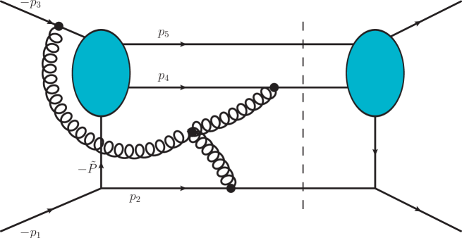
Figure 4: Squared amplitude with $n=5$ QCD partons in parton–parton hard scattering (the dashed line cuts the final-state partons). Representative colour structure of non-abelian factorization breaking correlations that accompany the two-parton SL collinear limit ($p_{i}\simeq z_{i}\widetilde{P},\;i=1,2$) at two-loop order.

We note that, in the case of a generic scattering amplitude with $n$ QCD partons, the colour structure of the contribution of ${\widetilde{\bf\Delta}}_{P}^{(2)}$ to ${\bf P}^{(2,R)}$ (see Eq. (181)) can be simplified. We have

$$\left({{\mbox{\boldmath$Sp$}}}^{(0,R)}\right)^{\dagger}\;{\widetilde{\bf\Delta}}_{P}^{(2)}(\epsilon)\;\;{{\mbox{\boldmath$Sp$}}}^{(0,R)}=\;{\overline{\bf\Delta}}_{P}^{(2)}(\epsilon)\;\;{\bf P}^{(0,R)}\;\;,$$ (193)

where the colour operator ${\overline{\bf\Delta}}_{P}^{(2)}$ acts on the colour space of the $n-1$ external QCD partons of the reduced matrix element ${\overline{\cal M}}$ (we recall that ${\bf P}^{(0,R)}$ is strictly factorized and, hence, it is proportional to the unit matrix in colour space). The simplified colour structure in Eq. (193) follows from the fact that we can explicitly evaluate the action of the colour charge ${{\mbox{\boldmath$T$}}}_{i}$ ($i=1,2$) of the collinear partons on the tree-level two-parton splitting matrix ${{\mbox{\boldmath$Sp$}}}^{(0,R)}$. Using basic colour algebra relations, we straightforwardly find ($i=1,2$)

$$\left({{\mbox{\boldmath$Sp$}}}^{(0,R)}(p_{1},p_{2};\widetilde{P})\right)^{\dagger}\;T_{i}^{a}\;{{\mbox{\boldmath$Sp$}}}^{(0,R)}(p_{1},p_{2};\widetilde{P})=\;T^{a}_{(i)\,\widetilde{P}}\;\;{\bf P}^{(0,R)}\;\;,$$ (194)

where the colour operator ${{\mbox{\boldmath$T$}}}_{(i)\,\widetilde{P}}$ is proportional to the colour charge of the parent collinear parton $A$ with momentum $\widetilde{P}$. The explicit expression of ${{\mbox{\boldmath$T$}}}_{(i)\,\widetilde{P}}$ depends on the flavour of the collinear parton $i$ and of the parent collinear parton. Considering the flavour structure of the various splitting processes $A\rightarrow A_{1}\,A_{2}$, we have

$${}\!\!\!\!f\rightarrow f\,g\;\;(f=q\;{\rm or}\;{\bar{q}}): \quad\;\;{{\mbox{\boldmath$T$}}}_{(f)\,f}=\left(1-\frac{C_{A}}{2C_{F}}\right)\;{{\mbox{\boldmath$T$}}}_{f}\;\;,\;\;\;\;{{\mbox{\boldmath$T$}}}_{(g)\,f}=\frac{C_{A}}{2C_{F}}\;{{\mbox{\boldmath$T$}}}_{f}\;\;,$$ (195)

$${}\!\!\!\!g\rightarrow g\,g\;: \quad\;\;{{\mbox{\boldmath$T$}}}_{(g)\,g}=\frac{1}{2}\;{{\mbox{\boldmath$T$}}}_{g}\;\;,$$ (196)

$${}\!\!\!\!g\rightarrow q\,{\bar{q}}\;: \quad\;\;{{\mbox{\boldmath$T$}}}_{(q)\,g}=\frac{1}{2}\;\left(\;{{\mbox{\boldmath$T$}}}_{g}+{{\mbox{\boldmath$d$}}}_{g}\right)\;\;,\;\;\;\;{{\mbox{\boldmath$T$}}}_{({\bar{q}})\,g}=\frac{1}{2}\;\left(\;{{\mbox{\boldmath$T$}}}_{g}-{{\mbox{\boldmath$d$}}}_{g}\right)\;\;,$$ (197)

where ${{\mbox{\boldmath$T$}}}_{f}$ and ${{\mbox{\boldmath$T$}}}_{g}$ are the customary colour charges of a fermion and a gluon, while ${{\mbox{\boldmath$d$}}}_{g}$ is the gluon colour matrix in a symmetric ‘octet’ state and its matrix elements are defined as

$$\left(d^{\,a}\right)_{bc}=\;d_{bac}\;\;,\quad d_{abc}\equiv 2\;{\rm Tr}\left(t^{a}\{t^{b},t^{c}\}\right)\;\;,$$ (198)

and $d_{abc}$ is the fully-symmetrized trace of $t^{a}t^{b}t^{c}$. The explicit expression of the colour operator ${\overline{\bf\Delta}}_{P}^{(2)}$ in Eq. (193) is

$${\overline{\bf\Delta}}_{P}^{(2)}(\epsilon) = \left(\frac{\alpha_{\mathrm{S}}(\mu^{2})}{2\pi}\right)^{2}\;\left(\frac{-s_{12}}{\mu^{2}}\right)^{\!\!-2\epsilon}2\;\pi\;f_{abc}\,\sum_{i=1,2}\;\sum_{\begin{subarray}{c}j,k=3\\ j\,\neq\,k\end{subarray}}^{n}\,T^{a}_{(i)\,\widetilde{P}}\,T_{j}^{b}\,T_{k}^{c}\;\Theta(-z_{i})\;{\rm sign}(s_{ij})\;\Theta(-s_{jk})$$ (199)

$$\times \ln\left(\,\frac{s_{j\widetilde{P}}\;s_{k\widetilde{P}}\,z_{1}z_{2}}{s_{jk}\,s_{12}}\right)\;\left[\,-\,\frac{1}{2\,\epsilon^{\,2}}\,+\frac{1}{\epsilon}\;\ln\left(\frac{-z_{i}}{1-z_{i}}\right)\right]\;\;.$$

This expression is directly obtained by inserting Eqs. (184) and (194) in the left-hand side of Eq. (193).

7.3 Multiparton collinear limit of squared amplitudes

In this subsection we consider the multiparton splitting $A\rightarrow A_{1}\dots A_{m}$ of $m$ ($m\geq 3$) collinear partons. The corresponding tree-level collinear matrix ${\bf P}^{(0,R)}$ fulfils strict factorization. The explicit expressions of ${\bf P}^{(0,R)}$ for all the flavour configurations of $m=3$ collinear partons were computed in Refs. [18, 19, 11].

The one-loop collinear matrix ${\bf P}^{(1,R)}$ is obtained by inserting Eqs. (96) and (97) in Eq. (170). We have

$${\bf P}^{(1,R)}=\left(\,{{\mbox{\boldmath$Sp$}}}^{(0,R)}\,\right)^{\dagger}\;{{\mbox{\boldmath$I$}}}^{(1)}_{m\,P}(\epsilon)\;{{\mbox{\boldmath$Sp$}}}^{(0,R)}+\left[\left(\,{{\mbox{\boldmath$Sp$}}}^{(0,R)}\,\right)^{\dagger}\,{{\mbox{\boldmath$Sp$}}}^{(1)\,{\rm fin.}}+\;{\rm h.c.}\;\right]\;\;,$$ (200)

where ${{\mbox{\boldmath$I$}}}^{(1)}_{m\,P}$ is given in terms of the colour operator ${{\mbox{\boldmath$I$}}}^{(1)}_{m\,C}$ in Eqs. (97) and (99):

$${{\mbox{\boldmath$I$}}}^{(1)}_{m\,P}(\epsilon)={{\mbox{\boldmath$I$}}}^{(1)}_{m\,C}(\epsilon)+\;{\rm h.c.}\;\;.$$ (201)

Using Eq. (99), the explicit expression of ${{\mbox{\boldmath$I$}}}^{(1)}_{m\,P}$ is

$${{\mbox{\boldmath$I$}}}^{(1)}_{m\,P}(\epsilon) = \frac{\alpha_{\mathrm{S}}(\mu^{2})}{2\pi}\;\left\{\left(\,\frac{1}{\epsilon^{2}}\,C_{\widetilde{P}}+\frac{1}{\epsilon}\,\gamma_{\widetilde{P}}\right)-\sum_{\begin{subarray}{c}i\,\in\,C\\ {}\end{subarray}}\left(\,\frac{1}{\epsilon^{2}}\,C_{i}+\frac{1}{\epsilon}\,\gamma_{i}-\,\frac{2}{\epsilon}\,C_{i}\,\ln|z_{i}|\right)\right.$$ (202)

$$- \frac{1}{\epsilon}\left.\sum_{\begin{subarray}{c}i,\ell\,\in C\\ i\,\neq\,\ell\end{subarray}}{{\mbox{\boldmath$T$}}}_{i}\cdot{{\mbox{\boldmath$T$}}}_{\ell}\,\ln\left(\frac{s_{i\ell}}{z_{i}\,z_{\ell}\,\mu^{2}}\right)\right\}\;\;.$$

The factorization breaking contribution ${{\mbox{\boldmath$\Delta$}}}^{(1)}_{m\,C}$ (see Eq. (100)) to ${{\mbox{\boldmath$I$}}}^{(1)}_{m\,C}$ is antihermitian and, thus, it cancels in Eq. (201). The operator ${{\mbox{\boldmath$I$}}}^{(1)}_{m\,P}$ depends on the colour charges of the collinear partons, but it is independent of the non-collinear partons. Therefore, the first term on the right-hand side of Eq. (200) does not violate strict collinear factorization. This term produces a strictly factorized and IR divergent contribution to ${\bf P}^{(1,R)}$.

The second term on the right-hand side of Eq. (200) is IR finite, since it depends on the IR finite contribution ${{\mbox{\boldmath$Sp$}}}^{(1)\,{\rm fin.}}$ to the one-loop splitting matrix. As mentioned in Sect. 5.3, ${{\mbox{\boldmath$Sp$}}}^{(1)\,{\rm fin.}}$ contains factorization breaking terms in the SL collinear region and, therefore, their interference with ${{\mbox{\boldmath$Sp$}}}^{(0,R)}$ can produce violation of strict collinear factorization at the squared amplitude level. In this respect, the main difference between the two-parton and multiparton collinear limits is that in the latter case several different colour structures contribute to the splitting matrix $Sp$ already at the tree level (in the two-parton case, ${{\mbox{\boldmath$Sp$}}}^{(0)}$ involves a single colour structure: see Eq. (16)). The result in Eqs. (200) and (202) for the multiparton collinear limit shows that the IR divergent part of ${\bf P}^{(1,R)}$ is strictly factorized, while the IR finite part can contain terms that produce violation of strict factorization in the squared amplitudes at the one-loop level (see Eq. (173)).

The two-loop collinear matrix ${\bf P}^{(2,R)}$ (see Eq. (171)) of the multiparton collinear limit can be computed by using Eqs. (96), (97), (156), (157) and the explicit form of the colour operators ${{\mbox{\boldmath$I$}}}^{(1)}_{m\,C}$ and ${{\mbox{\boldmath$I$}}}^{(2)}_{m\,C}$ (see Eqs. (99) and (158)). Performing some straightforward (though, slightly cumbersome) algebraic operations, we can write the result in the following form:

$${\bf P}^{(2,R)}={\bf P}^{(2,R)}_{\rm f.}+{\bf P}^{(2,R)}_{\rm n.f.}\;\;,$$ (203)

where the contribution ${\bf P}^{(2,R)}_{\rm f.}$ is strictly factorized, while the term ${\bf P}^{(2,R)}_{\rm n.f.}$ includes all the contributions that violate strict collinear factorization (this term also includes additional contributions that are strictly factorized).

The strictly-factorized term ${\bf P}^{(2,R)}_{\rm f.}$ does not depend on the non-collinear partons. Its explicit expression is

$${\bf P}^{(2,R)}_{\rm f.} = \left(\,{{\mbox{\boldmath$Sp$}}}^{(0,R)}\,\right)^{\dagger}\left\{\left[\,\frac{1}{2}\;{{\mbox{\boldmath$I$}}}^{(1)}_{m\,P}(\epsilon)\,{{\mbox{\boldmath$I$}}}^{(1)}_{m\,C,\,{\rm f.}}(\epsilon)+\;{\rm h.c.}\;\right]\right.$$ (204)

$$+ \left.\frac{\alpha_{\mathrm{S}}(\mu^{2})}{2\pi}\left(\,\frac{1}{\epsilon}\,b_{0}\left[{{\mbox{\boldmath$I$}}}^{(1)}_{m\,P}(2\epsilon)-{{\mbox{\boldmath$I$}}}^{(1)}_{m\,P}(\epsilon)\right]+K\;{{\mbox{\boldmath$I$}}}^{(1)}_{m\,P}(2\epsilon)\right)\right.$$

$$+ \,\left(\frac{\alpha_{\mathrm{S}}(\mu^{2})}{2\pi}\right)^{2}\left.\left.\,\frac{2}{\epsilon}\;\Bigl{(}\;\sum_{i\,\in C}\,H^{(2)}_{i}\Bigr{.}\Bigl{.}-H^{(2)}_{\widetilde{P}}\right.\Bigr{)}\right\}\;{{\mbox{\boldmath$Sp$}}}^{(0,R)}$$

where ${{\mbox{\boldmath$I$}}}^{(1)}_{m\,P}$ is the one-loop operator in Eq. (202), and the colour operator ${{\mbox{\boldmath$I$}}}^{(1)}_{m\,C,\,{\rm f.}}$ is obtained from ${{\mbox{\boldmath$I$}}}^{(1)}_{m\,C}$ (see Eq. (99)) by removing its factorization breaking part ${{\mbox{\boldmath$\Delta$}}}^{(1)}_{m\,C}$:

$${{\mbox{\boldmath$I$}}}^{(1)}_{m\,C,\,{\rm f.}}(\epsilon)={{\mbox{\boldmath$I$}}}^{(1)}_{m\,C}(\epsilon)-{{\mbox{\boldmath$\Delta$}}}^{(1)}_{m\,C}(\epsilon)\;\;.$$ (205)

The contribution ${\bf P}^{(2,R)}_{\rm n.f.}$ on the right-hand side of Eq. (203) has the following expression:

$${\bf P}^{(2,R)}_{\rm n.f.} = \left(\,{{\mbox{\boldmath$Sp$}}}^{(0,R)}\,\right)^{\dagger}\;{\bf\Delta}_{m\,P}^{(2;\,2)}(\epsilon)\;{{\mbox{\boldmath$Sp$}}}^{(0,R)}$$ (206)

$$+ \left[\left(\,{{\mbox{\boldmath$Sp$}}}^{(0,R)}\,\right)^{\dagger}\left(\,{{\mbox{\boldmath$I$}}}^{(1)}_{m\,P}(\epsilon)\;{{\mbox{\boldmath$Sp$}}}^{(1)\,{\rm fin.}}+{\overline{{\mbox{\boldmath$Sp$}}}}^{(2)\,{\rm div.}}+{{\mbox{\boldmath$Sp$}}}^{(2)\,{\rm fin.}}\,\right)+\;{\rm h.c.}\;\right]$$

$$+ \left(\,{{\mbox{\boldmath$Sp$}}}^{(1)\,{\rm fin.}}\,\right)^{\dagger}\;{{\mbox{\boldmath$Sp$}}}^{(1)\,{\rm fin.}}\;\;,$$

where the colour operator ${\bf\Delta}_{m\,P}^{(2;\,2)}$ is

$${\bf\Delta}_{m\,P}^{(2;\,2)}(\epsilon)=\left(\,{\bf\Delta}_{m\,C}^{(2;\,2)}(\epsilon)+\;{\rm h.c.}\;\right)+\frac{1}{2}\left[\;{{\mbox{\boldmath$I$}}}^{(1)}_{m\,P}(\epsilon),\;{{\mbox{\boldmath$\Delta$}}}^{(1)}_{m\,C}(\epsilon)\;\right]\;\;.$$ (207)

The last term on the right-hand side of Eq. (206) is IR finite, since it is given by the square of the IR finite contribution ${{\mbox{\boldmath$Sp$}}}^{(1)\,{\rm fin.}}$ to the one-loop splitting matrix (see Eq. (96)). As already recalled, ${{\mbox{\boldmath$Sp$}}}^{(1)\,{\rm fin.}}$ contains factorization breaking terms in the SL collinear region.

The term in the square bracket on the right-hand side of Eq. (206) is IR divergent. This term depends on ${{\mbox{\boldmath$Sp$}}}^{(1)\,{\rm fin.}}$, on the colour operator ${{\mbox{\boldmath$I$}}}^{(1)}_{m\,P}$ in Eq. (202), and on the contributions ${{\mbox{\boldmath$Sp$}}}^{(2)\,{\rm fin.}}$ (see Eq. (156)) and ${\overline{{\mbox{\boldmath$Sp$}}}}^{(2)\,{\rm div.}}$ (see Eq. (157)) to the two-loop splitting matrix ${{\mbox{\boldmath$Sp$}}}^{(2,R)}$. As stated in Sect. 6.3, ${\overline{{\mbox{\boldmath$Sp$}}}}^{(2)\,{\rm div.}}$ contains factorization breaking contributions that are IR divergent at the level of single poles $1/\epsilon$. The operator ${{\mbox{\boldmath$I$}}}^{(1)}_{m\,P}$ contains also a double-pole term with a $c$-number coefficient (see Eq. (202)) and, thus, it produces the following IR divergent contribution to the square-bracket term in Eq. (206):

$$\left({{\mbox{\boldmath$Sp$}}}^{(0,R)}\,\right)^{\dagger}\!{{\mbox{\boldmath$I$}}}^{(1)}_{m\,P}(\epsilon)\,{{\mbox{\boldmath$Sp$}}}^{(1)\,{\rm fin.}}+\,{\rm h.c.}\!\!\! = \!\!\!\frac{\alpha_{\mathrm{S}}(\mu^{2})}{2\pi}\Bigl{(}C_{\widetilde{P}}-\sum_{\begin{subarray}{c}i\,\in\,C\\ {}\end{subarray}}C_{i}\Bigr{)}\frac{1}{\epsilon^{2}}\left[\left({{\mbox{\boldmath$Sp$}}}^{(0,R)}\,\right)^{\dagger}\!{{\mbox{\boldmath$Sp$}}}^{(1)\,{\rm fin.}}+\;{\rm h.c.}\right]$$ (208)

$$+ \!\!\!{\cal O}(1/\epsilon)\;\;.$$

We note that the double-pole term in Eq. (208) is simply proportional to the factorization breaking contribution to the one-loop collinear matrix ${\bf P}^{(1,R)}$ (see Eq. (200)).

The colour operator ${\bf\Delta}_{m\,P}^{(2;\,2)}$ in Eq. (207) depends on the two-loop factorization breaking term ${\bf\Delta}_{m\,C}^{(2;\,2)}$ (see Eqs. (158) and (159)), on the one-loop operator ${{\mbox{\boldmath$I$}}}^{(1)}_{m\,P}(\epsilon)$, and on the one-loop factorization breaking term ${{\mbox{\boldmath$\Delta$}}}^{(1)}_{m\,C}$ (see Eqs. (99) and (100)). The commutator on the right-hand side of Eq. (207) originates from a non-abelian interference of two types of one-loop contributions: the one-loop absorptive (antihermitian) contribution to the scattering amplitude (the absorptive interaction involves a collinear and a non-collinear parton) and the one-loop radiative (hermitian) contribution to the complex conjugate amplitude (the radiative interaction involves two collinear partons). Using Eqs. (100) and (202), we evaluate the commutator and we obtain the following explicit expression of ${\bf\Delta}_{m\,P}^{(2;\,2)}$:

$${\bf\Delta}_{m\,P}^{(2;\,2)}(\epsilon) = \!\!\left(\frac{\alpha_{\mathrm{S}}(\mu^{2})}{2\pi}\right)^{2}\left(\,-\,\frac{1}{\epsilon^{2}}\right)\;\pi\;f_{abc}$$ (209)

$$\times \!\!\left[\;\sum_{i\in C}\;\sum_{\begin{subarray}{c}j,k\,\in NC\\ j\,\neq\,k\end{subarray}}\,T_{i}^{a}\,T_{j}^{b}\,T_{k}^{c}\;\Theta(-z_{i})\;{\rm sign}(s_{ij})\;\Theta(-s_{jk})\;\ln\left(\,\frac{s_{j\widetilde{P}}\;s_{k\widetilde{P}}}{s_{jk}\,\mu_{0}^{2}}\right)\right.$$

$$- \left.\;\sum_{\begin{subarray}{c}i,\ell\,\in C\\ i\,\neq\,\ell\end{subarray}}\;\sum_{j\in NC}\;\,T_{i}^{a}\,T_{\ell}^{b}\,T_{j}^{c}\;\Theta(-z_{i})\;\Theta(-s_{i\ell})\;{\rm sign}(s_{ij})\;\,\ln\left(\,\frac{s_{i\ell}}{z_{i}z_{\ell}\,\mu_{0}^{2}}\right)\;\right].$$

Note that the argument of the logarithms in the square bracket depends on the scale $\mu_{0}$, which is arbitrary (we can possibly set $\mu_{0}=\mu$). However, the expression (209) is actually independent of $\mu_{0}$; the independence of $\mu_{0}$ directly follows from the relation (162) (to apply Eq. (162), we note that the explicit constraint $s_{i\ell}<0$ can be removed from the second term in the square bracket of Eq. (209); indeed, the sum of the terms with $s_{i\ell}>0$ gives a vanishing contribution to Eq. (209)).

The operator ${\bf\Delta}_{m\,P}^{(2;\,2)}$ is IR divergent and proportional to the double pole $1/\epsilon^{2}$. The first term in the square bracket of Eq. (209) involves non-abelian contributions that correlate the colour charges of two non-collinear partons (and a collinear parton). In Eq. (206), these contributions produce factorization breaking terms that cannot be cancelled by the IR divergent term of Eq. (208) (indeed, as mentioned in Sect. 5.3, ${{\mbox{\boldmath$Sp$}}}^{(1)\,{\rm fin.}}$ embodies factorization breaking correlations with a single non-collinear parton). Therefore, the explicit expression (209) of ${\bf\Delta}_{m\,P}^{(2;\,2)}$ shows that the two-loop multiparton collinear matrix ${\bf P}^{(2,R)}$ necessarily includes non-abelian contributions that lead to violation of strict collinear factorization at the squared amplitude level.

A special exception to this conclusion about violation of strict collinear factorization regards the case of the SL collinear limit in lepton–hadron DIS. In the DIS case, the operator ${\bf\Delta}_{m\,P}^{(2;\,2)}$ effectively takes a form that is independent of the non-collinear partons. To show this, we consider a DIS matrix element ${\cal M}(p_{1},\dots,p_{m},p_{m+1},\dots,p_{n})$: the initial-state parton has ‘outgoing’ momentum $-p_{1}$ ($p_{1}^{0}<0$), the momenta of the final-state collinear partons are $p_{2},\dots,p_{m}$, and the momenta of the final-state non-collinear partons are $p_{m+1},\dots,p_{n}$. If $j,k\in NC$, we have $s_{jk}>0$: thus, the correlation terms of Eq. (209) that depend on two non-collinear partons vanish. As for the remaining correlation terms of Eq. (209), the sign of $s_{ij}$ is independent of $j$ if $j\in NC$ (actually, $s_{ij}>0$ if $i\in C$ and $z_{i}<0$); therefore, we can perform the sum over $j$ by using colour conservation $(\sum_{j\in NC}{{\mbox{\boldmath$T$}}}_{j}=-\sum_{r\in C}{{\mbox{\boldmath$T$}}}_{r})$. The final expression of ${\bf\Delta}_{m\,P}^{(2;\,2)}$ in lepton–hadron DIS is

$${\bf\Delta}_{m\,P}^{(2;\,2)}(\epsilon) = \!\!\left(\frac{\alpha_{\mathrm{S}}(\mu^{2})}{2\pi}\right)^{2}\left(\,-\,\frac{1}{\epsilon^{2}}\right)\;\pi\;f_{abc}$$ (210)

$$\times \!\!\;\sum_{\begin{subarray}{c}i,\ell\,\in C\\ i\,\neq\,\ell\end{subarray}}\;\,T_{i}^{a}\,T_{\ell}^{b}\;\sum_{r\in C}\,T_{r}^{c}\;\Theta(-z_{i})\;\Theta(-s_{i\ell})\;\,\ln\left(\,\frac{s_{i\ell}}{z_{i}z_{\ell}\,\mu_{0}^{2}}\right)\;,\quad({\rm DIS})\;.$$

This expression is independent of the non-collinear partons and, thus, it effectively has a strictly-factorized form. This form is a consequence of a colour coherence mechanism (due to DIS kinematics and colour conservation).

In generic kinematical configurations (typically, those that occur in hadron–hadron hard-scattering processes), the two-loop multiparton collinear matrix ${\bf P}^{(2,R)}$ is not strictly factorized. We note that the two-loop collinear formula (174) for the squared amplitudes includes factorization breaking contributions that are due to both ${\bf P}^{(1,R)}$ and ${\bf P}^{(2,R)}$. The factorization breaking contributions that are due to ${\bf P}^{(1,R)}$ involve correlations with one non-collinear parton, while the contributions due to ${\bf P}^{(2,R)}$ also involve correlations with two non-collinear partons.

7.4 Cross sections and violation of strict collinear factorization: some remarks

The applicability of perturbative QCD to the calculation of cross sections for hard-scattering processes is based on the universal (process-independent) factorization theorem of mass singularities [29]. According to this factorization picture, the sole uncancelled IR divergences that are eventually encountered in the computation of inclusive partonic cross sections are due to partonic states whose momenta are collinear to the momenta of the colliding partons or of triggered final-state partons; these uncancelled divergences are factorizable in a process-independent form and, therefore, they can be removed by a formal redefinition (‘renormalization’) of the ‘bare’ parton densities and parton fragmentation functions.

The violation of strict collinear factorization at the level of squared amplitudes certainly challenges the validity of universal mass-singularity factorization at the cross section level. We present some comments and remarks on this issue.

We first present a general comment. The singular behaviour of the two-parton collinear limit at one-loop order is one of the key ingredients that are used to handle IR divergences and mass singularities and to cancel the IR divergences in perturbative QCD computations of hard-scattering processes at the NNLO (see, e.g., Refs. [57, 58, 59, 60, 61, 56, 62, 63] and references therein). In this context, it is reassuring that the one-loop two-parton collinear matrix ${\bf P}^{(1,R)}$ is strictly factorized even in the SL collinear region (see Eqs. (178)–(180)). This result guarantees that the extension of NNLO methods from lepton–lepton collisions to lepton–hadron and hadron–hadron collisions does not involve additional conceptual difficulties related to the violation of strict collinear factorization.

In the following, rather than considering the issue of mass-singularity factorization in completely general terms, we limit our discussion to the simplest case in which our study has definitely uncovered the presence of strict-factorization breaking effects at the squared amplitude level. We thus consider the inclusive production of a high-$p_{T}$ hadron or jet (with at least one recoiling jet) in the collision between two high-energy hadrons.

At the leading order (LO) in QCD perturbation theory, this production process is controlled by the square of the tree-level amplitude (with $n=4$ partons) of the corresponding partonic subprocess

$${\rm~{}parton+parton}\rightarrow 2~{}{\rm partons~{}}\;\;.$$ (211)

Part of the higher-order QCD corrections to this ‘$2\rightarrow 2$’ partonic subprocess are obtained by considering the squared amplitude of the process

$${\rm~{}parton+parton}\rightarrow 3~{}{\rm partons~{}}\;\;,\quad\;\;({\rm one\;low-}p_{T}\;\,{\rm final\!-\!state\;parton})\;,$$ (212)

in the kinematical region where one of the three final-state partons (the ‘low-$p_{T}$ parton’) is collinear to one of the initial-state partons. The IR divergences produced by the phase space integration over the SL collinear region of the low-$p_{T}$ final-state parton have to be factorized with respect to the corresponding LO ‘$2\rightarrow 2$’ partonic subprocess, and the IR factor has to be strictly factorized, namely, it has to be independent of the kinematical and colour flow structures of the LO partonic subprocess in Eq. (211). As explicitly shown in Sect. 7.2, the squared amplitude of the process in Eq. (212) violates strict factorization in the SL collinear region. This violation of strict factorization starts at the two-loop level (see Eqs. (181) and (192), and Fig. 4) and, therefore, it may invalidate the factorization theorem of mass singularities starting at the N³LO in QCD perturbation theory. The validity of the factorization theorem can be recovered only if the N³LO factorization breaking effects produced by the two-parton SL collinear limit of the process in Eq. (212) are cancelled by corresponding factorization breaking effects produced by other partonic subprocesses. An explicit quantitative proof of such a cancellation would represent a highly non-trivial check of the validity of the factorization theorem beyond the NNLO.

We continue our discussion of the cancellation mechanism at the qualitative level and, eventually, we shall identify a sole additional partonic configuration that can lead to factorization breaking correlations with the same structure as in Eq. (192) (see Fig. 4). The contribution of this partonic configuration (after combination with all the other IR divergent terms) can cancel the violation of strict collinear factorization that is produced by the subprocess in Eq. (212).

To reach this conclusion, we consider the various high-order subprocesses that lead to the N³LO IR divergent contributions to the cross section controlled by the LO process in Eq. (211), and we group them in three classes: $i)$ virtual and soft-parton subprocesses, $ii)$ collinear-parton subprocesses, and $iii)$ mixed soft-collinear parton subprocesses.

The class $\,i)$ contains the virtual three-loop corrections to the ‘$2\rightarrow 2$’ process in Eq. (211) and the $(3-k)$-loop corrections to the processes ‘parton + parton $\rightarrow$ 2 partons + $k$ soft partons’ with $k=1,2,3$. Owing to kinematics, the IR divergences produced by this class cannot cancel the factorization breaking effects due to the two-loop corrections of the process in Eq. (212). In fact, the virtual and soft-parton radiation that accompanies the basic ‘$2\rightarrow 2$’ partonic process cannot match the kinematics of the process ‘parton + parton $\rightarrow$ 3 partons’ in the region where the final-state collinear parton has a large longitudinal-momentum fraction (e.g., $p_{2}\simeq z_{2}\widetilde{P}$ with $|z_{2}|\sim|z_{1}|\sim{\cal O}(1)$ in Eqs. (181) and (192), and in Fig. 4). The subprocesses of the class $\,i)\,$ can (partly) cancel the IR divergences of the subprocess in Eq. (212) only in the kinematical region where the final-state collinear parton is also soft (e.g., at the kinematical endpoint $z_{1}=1-z_{2}\rightarrow 1$ in Eq. (181)).

The class $\,ii)$ contains the subprocess in Eq. (212) at the two-loop level and two other contributions: the tree-level subprocess ‘parton + parton $\rightarrow$ 5 partons’ with three low-$p_{T}$ final-state partons, and the one-loop subprocess ‘parton + parton $\rightarrow$ 4 partons’ with two low-$p_{T}$ final-state partons. The subprocess ‘parton + parton $\rightarrow$ 5 partons’ produces IR divergent terms from the tree-level SL collinear limit of $m=4$ partons: this tree-level collinear limit is strictly factorized. The subprocess

$${\rm~{}parton+parton}\rightarrow 4~{}{\rm partons~{}}\;\;\quad\;\;({\rm two\;low-}p_{T}\;\,{\rm final\!-\!state\;partons})\;$$ (213)

produces IR divergent terms from the one-loop SL collinear limit of $m=3$ partons: this collinear limit violates strict factorization but, as discussed in Sects. 5.1, 5.3 and 7.3 (see Eq. (200)), the corresponding factorization breaking terms involve correlations with a single non-collinear parton. Since the factorization breaking effects due to the two-loop subprocess in Eq. (212) also involve correlations with two non-collinear partons (see Eq. (192) and Fig. 4), these effects cannot be fully cancelled by the contributions of the other subprocesses in the class $\,ii)$.

The class $\,iii)$ contains two tree-level subprocesses: the subprocess ‘parton + parton $\rightarrow$ 4 partons + $1$ soft parton’, which produces IR divergent terms from the SL collinear limit of $m=3$ partons (two of the non-soft final-state partons have low $p_{T}$), and the subprocess ‘parton + parton $\rightarrow$ 3 partons + $2$ soft partons’, which contributes through the SL collinear limit of $m=2$ partons (one of the non-soft final-state partons has low $p_{T}$). Owing to colour coherence (see Sects. 3.4 and 3.5 in Ref. [11]), the singular collinear factors are strictly factorized in these mixed soft-collinear limits of tree-level QCD amplitudes. The remaining contribution to the class $\,iii)$ is due to the subprocess

$${\rm~{}parton+parton}\rightarrow 3~{}{\rm partons+1~{}soft\;parton~{}}\;\;,\quad\;\;({\rm one\;low-}p_{T}\;\,{\rm final\!-\!state\;parton})\;,$$ (214)

in the kinematical region where one of the three non-soft final-state partons is collinear to one of the initial-state partons (Fig. 5). The subprocess in Eq. (214) contributes to one-loop order. The structure of the absorptive part of the one-loop interaction limits the coherent action of the two collinear partons in the SL region (the mechanism is analogous to that discussed in Sect. 4.5). As a consequence, the one-loop mixed soft-collinear limit of the process in Eq. (214) leads to a singular SL collinear factor that violates strict factorization. Moreover, this singular factor can also produce correlations with two non-collinear partons (see Fig. 5), whose structure is analogous to that in Eqs. (181) and (192) (see Fig. 4).

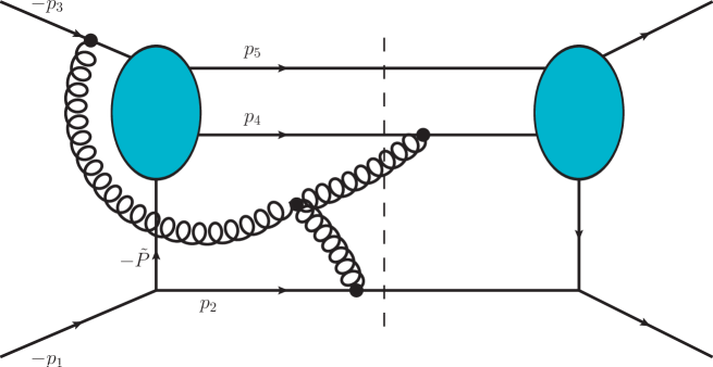
Figure 5: Squared amplitude for parton–parton hard-scattering with three QCD partons and one soft gluon in the final state (the dashed line cuts the final-state partons). Representative colour structure of non-abelian factorization breaking correlations that accompany the mixed soft-collinear limit (with two collinear partons, $p_{i}\simeq z_{i}\widetilde{P},\;i=1,2$, in the SL region) at one-loop order.

In summary, the two-loop radiative corrections to the subprocess in Eq. (212) and the one-loop radiative corrections to the subprocesses in Eqs. (213) and (214) produce violation of strict factorization in the SL collinear region. The factorization breaking effects are due to the singular partonic configurations with $m=2$ collinear partons, $m=3$ collinear partons, and $m=2$ collinear partons plus one radiated soft parton. The factorization breaking terms involve correlations with one and two (in the case of the subprocesses in Eqs. (212) and (214)) hard non-collinear partons.

In the inclusive hadroproduction of a single high-$p_{T}$ jet (or hadron), this violation of strict collinear factorization leads to N³LO contributions that are separately IR divergent; the total contribution of these IR divergent terms should vanish to guarantee the validity of the factorization theorem of mass singularities.

Even if the IR cancellation occurs, the violation of strict collinear factorization leads to residual IR finite terms. These terms can produce observable contributions that are logarithmically enhanced (and, therefore, large) in particular kinematical configurations where virtual (see Eq. (212)) and real (see Eqs. (213) and (214)) radiative corrections are highly unbalanced. For instance, in these kinematical configurations the cancellation of the IR pole term of ${\cal O}(1/\epsilon^{2})$ in Eq. (192) can lead to a residual double-logarithmic contribution. The logarithmically-enhanced terms due to the violation of strict collinear factorization have a distinctive signature: the factorization breaking correlations with the non-collinear partons (see, e.g., Eq. (192) and Figs. 4 and 5) produce ‘entangled logarithms’, namely, logarithmic terms whose coefficients get tangled up with the colour flow and kinematical structure of the lowest-order hard-scattering subprocess (e.g., Eq. (211)). In the following, we mention some specific examples of processes that can exhibit entangled logarithms at various perturbative orders.

The partonic subprocess in Eq. (211) also controls the LO inclusive hadroproduction of a pair of nearly back-to-back high-$p_{T}$ hadrons or jets. In the kinematical region where the total transverse momentum ${\bf Q}_{T}$ of the pair is small (e.g., much smaller than the invariant mass of the pair), the perturbative QCD calculation leads to large contributions that are proportional to powers of $\ln Q_{T}$. Owing to the violation of strict collinear factorization in the subprocesses of Eqs. (212)–(214), part of these logarithmic contributions can be due to entangled logarithms (the entangled logarithms are absent if the small-$Q_{T}$ triggered final-state system includes no QCD partons [64, 53]) that first appear at the N³LO. The presence of these small-$Q_{T}$ entangled logarithms is also related to issues that arise in the context of factorization of transverse-momentum dependent distributions [30, 31, 32].

The perturbative QCD calculation of the inclusive hadroproduction of three high-$p_{T}$ jets is also affected by large logarithms, $\ln p_{T}^{\,\rm min}$, in the kinematical region where the transverse momentum $p_{T}^{\,\rm min}$ of the lowest-$p_{T}$ jet is small (e.g., much smaller than the transverse momenta of the other two jets). In this three-jet production process, the partonic subprocess in Eq. (212) enters at the LO, and the partonic subprocesses in Eqs. (213) and (214) first contribute at the NLO. The two-loop (in the case of the subprocess in Eq. (212)) and one-loop (in the case of the subprocesses in Eqs. (213) and (214)) violation of strict collinear factorization can produce small-$p_{T}^{\,\rm min}$ entangled logarithms starting from the NNLO perturbative calculation.

Another example of entangled logarithms is represented by the super-leading (‘non-global’) logarithmic terms discovered [33] in the calculation of the cross section for the hadroproduction of a pair of jets with a rapidity gap between them. These super-leading logarithms occur at the N⁴LO in QCD perturbation theory.

8 Summary

We have studied the singular behaviour of QCD scattering amplitudes in the kinematical configurations where the momenta of two or more external partons become collinear. We have shown that, beyond the tree-level, strict (process-independent) collinear factorization is violated in the SL collinear region. We have introduced a generalized form of collinear factorization (see Eq. (33) in Sect. 4.1, and Eqs. (78) and (5.2) in Sect. 5.2) of the all-order scattering amplitudes, which is valid in both the TL and SL collinear regions. In the SL region, the singular collinear factor retains some process dependence, since it depends on the momenta and colour charges of the non-collinear partons. Owing to this colour dependence, the formulation of collinear factorization directly in colour space, through the use of collinear splitting matrices, is particularly suitable. An equivalent formulation in terms of colour subamplitudes and collinear splitting amplitudes is feasible (see Appendix A). In the TL collinear region, strict factorization is recovered because of colour coherence. In the SL collinear region, colour coherence is limited by the causality structure of long-range gauge interactions (roughly, the distinction between initial-state and final-state interactions), and this produces absorptive contributions that eventually originate in the strict-factorization breaking phenomenon (see Sect. 4.5).

In the case of the two-parton SL collinear limit, we have computed the ($d$-dimensional) one-loop splitting matrix (Eqs. (4.1) and (4.1)) to all orders in the dimensional regularization parameter $\epsilon$. The SL result explicitly shows that it cannot be obtained from the previously known TL result by using crossing symmetry. The strict-factorization breaking terms are antihermitian (‘imaginary’) at one-loop level. The expressions in Eqs. (52) and (67), which refer to the SL collinear limit in hadron–hadron collisions, are the simplest examples of terms that violate strict collinear factorization. At two-loop level (Sect. 6.2), we have explicitly computed all the IR divergent contributions (i.e., the $\epsilon$ poles) to the splitting matrix. The two-loop result shows the presence of both hermitian (‘real’) and antihermitian terms that violate strict collinear factorization.

We have derived the structure of the IR divergences of the multiparton collinear limit to all orders in the loop expansion (Sect. 6.1). We have explicitly computed one-loop (Sect. 5.3) and two-loop (Sect. 6.3) IR divergent contributions to the SL collinear limit of $m\geq 3$ partons, thus extending the results of the two-parton collinear limit.

The SL collinear limit of the scattering amplitudes that are involved in lepton–hadron DIS (namely, parton radiation collinear to the sole initial-state parton) is a special case, since all the non-collinear partons are produced in the final state. The one-loop expression of the two-parton SL splitting matrix ‘effectively’ takes a strictly-factorized form, in which there is no explicit dependence on the non-collinear partons (see Sect. 4.4). This effective strict factorization of the SL collinear limit can be a general feature of the DIS kinematics (there are no initial-state interactions between collinear and non-collinear partons). The one-loop and two-loop terms of the multiparton splitting matrix that we have explicitly computed fulfill this effective strict factorization in the DIS kinematical configuration.

In hadron–hadron collision configurations, the two-loop SL splitting matrix has factorization breaking terms that are definitely non-abelian (see Sects. 6.2 and 6.3). These terms involve correlations between the momenta and colour charges of three partons and, in particular, between a collinear parton and two non-collinear partons. These non-abelian factorization breaking effects appear in the SL collinear limit of two-loop scattering amplitudes with at least five external legs and, in particular, $n\geq 4$ external QCD partons.

Owing to their absorptive origin, strict-factorization breaking effects partly cancel at the level of squared amplitudes. Nonetheless, strict factorization is certainly violated in the SL collinear limit of two-loop squared amplitudes for parton–parton hard scattering with at least three final-state partons (see Sect. 7.2 and, in particular, Eq. (192)). These factorization breaking effects have consequences in perturbative QCD calculations of hard-scattering cross sections in hadron–hadron collisions (Sect. 7.4). The violation of strict factorization affects the non-abelian structure of logarithmically-enhanced terms at NNLO and higher orders; it has implications on various factorization issues and, in particular, it challenges the validity of mass-singularity factorization in jet and hadron production, starting from the N³LO.

Appendix A Appendix: Multigluon amplitudes and the structure of the collinear limit

In this Appendix we consider the specific case in which the matrix element ${\cal M}(p_{1},p_{2},\dots,p_{n})$ is a multiparton scattering amplitude with $n$ external gluons. We recall the decomposition of the matrix element in colour subamplitudes, and we illustrate the behaviour of the colour subamplitudes in the collinear limit.

The colour indices of the $n$ external gluons of ${\cal M}(p_{1},\dots,p_{n})$ are denoted by $a_{1},\dots,a_{n}$. At the tree level the pure multigluon amplitude ${\cal M}^{(0)}$ (see Eq. (1)) can be expressed as follows [17]

$${\cal M}^{(0)\,a_{1},\dots,a_{n}}(p_{1},\dots,p_{n})=(\sqrt{2})^{n}\;{\rm Tr}\left(t^{a_{1}}\dots t^{a_{n}}\right)\;{\cal A}^{(0)}(1,\dots,n)+{\rm non-}{\rm cyclic\;perms.}\;\;,$$ (215)

where $t^{a_{i}}$’s are colour matrices in the fundamental representation (see Eq. (11)), and the sum of terms on the right-hand side extends over the $(n-1)!$ non-cyclic permutations of the set $\{1,2,\dots,n\}$ of the external legs. This is the customary colour decomposition in colour subamplitudes. Each tree-level colour subamplitude, ${\cal A}^{(0)}(1,\dots,n)$, is independent of the colour indices, and it embodies the kinematical dependence on the momenta and spin polarizations of the external gluons. Note, however, that the colour subamplitudes are colour ordered, namely, the functional form of ${\cal A}^{(0)}(1,\dots,i,\dots,j,\dots,n)$ depends on the specific ordering $(1,\dots,i,\dots,j,\dots,n)$ of the external legs in the argument of ${\cal A}^{(0)}$ (e.g., ${\cal A}^{(0)}(1,\dots,i,\dots,j,\dots,n)\neq{\cal A}^{(0)}(1,\dots,j,\dots,i,\dots,n)$). The overall normalization of the colour subamplitudes in Eq. (215) is adjusted to that used in Refs. [12, 25]; the only difference between ${\cal A}^{(0)}(1,\dots,n)$ and the corresponding subamplitude $A_{n}^{\rm tree}(1,\dots,n)$ in Refs. [12, 25] is due to the overall factor $g_{\mathrm{S}}^{n-2}$, which we have included in the definition of ${\cal A}^{(0)}(1,\dots,n)$.

At the one-loop level the colour structure of the multigluon amplitude ${\cal M}^{(1)}$ (see Eq. (1)) is [65, 12, 25]

$${\cal M}^{(1)\,a_{1},\dots,a_{n}}(p_{1},\dots,p_{n}) \!\!=\!\! \left\{(\sqrt{2})^{n}\;{\rm Tr}\left(t^{a_{1}}\dots t^{a_{n}}\right)\;{\cal A}^{(1)}(1,\dots,n)+{\rm non-}{\rm cyclic\;perms.}\right\}$$ (216)

$$\!\!+\!\! {\rm double\;trace\;terms}\;\;.$$

The term in the curly bracket has the same colour structure of Eq. (215). The subamplitude ${\cal A}^{(1)}(1,\dots,n)$, which is called leading-colour subamplitude (or primitive amplitude), is the one-loop analogue of the tree-level colour subamplitude ${\cal A}^{(0)}(1,\dots,n)$. The remaining terms on the right-hand side of Eq. (216) are proportional to colour factors that involve the product of two traces of $t^{a}$ matrices, namely, ${\rm Tr}\left(t^{a_{1}}\dots t^{a_{k}}\right)\,{\rm Tr}\left(t^{a_{k+1}}\dots t^{a_{n}}\right)$. Each double trace is multiplied by a corresponding kinematical factor called subleading-colour subamplitude (or subleading-colour ‘partial amplitude’). The subleading-colour partial amplitudes are in fact not independent of the leading-colour subamplitudes ${\cal A}^{(1)}(1,\dots,n)$; rather, they can be expressed as sum over permutations of the arguments of the latter. Owing to this linear dependence, it suffices to examine the collinear limit of the leading-colour subamplitudes. In particular, we do not explicitly consider subleading-colour partial amplitudes and their contribution to Eq. (216).

As in the case of the tree-level colour decomposition in Eq. (215), our normalization of the one-loop subamplitude ${\cal A}^{(1)}(1,\dots,n)$ is adjusted to that used in Refs. [12, 25]. To be precise, at the one-loop level the authors of Refs. [12, 25] decompose the QCD leading-colour subamplitude in two terms, $A_{n}^{{\rm 1-loop}\,[1]}$ and $A_{n}^{{\rm 1-loop}\,[1/2]}$: the subscripts $[1]$ and $[1/2]$ respectively refer to the contribution of a gluon and a quark circulating in the loop. The relation between our ${\cal A}^{(1)}(1,\dots,n)$ and the subamplitudes of Ref. [12] is ${\cal A}^{(1)}(1,\dots,n)=g_{\mathrm{S}}^{n}[N_{c}\,A_{n}^{{\rm 1-loop}\,[1]}(1,\dots,n)+N_{f}\,A_{n}^{{\rm 1-loop}\,[1/2]}(1,\dots,n)]$.

To present the collinear behaviour of the colour subamplitudes, we first explicitly relate the colour matrix ${{{\mbox{\boldmath$Sp$}}}}_{g_{1}g_{2}}$ of the splitting process $g\rightarrow g_{1}g_{2}$ to its colour stripped component, the splitting amplitude ${\rm Split}$ (see Eq. (16)). At the tree level we define:

$$Sp_{g_{1}g_{2}}^{(0)\;(a_{1},a_{2};\,a)}(p_{1},p_{2};{\widetilde{P}})\equiv{\sqrt{2}}\;\;i\;f_{a_{1}a_{2}\,a}\;\,{\rm Split}^{(0)}(p_{1},p_{2};\widetilde{P})\;\;,$$ (217)

where the explicit expression of ${\rm Split}^{(0)}$ can be extracted by direct inspection of Eq. (2). Analogously, at the one-loop level we consider the splitting matrix ${{\mbox{\boldmath$Sp$}}}^{(1)}_{H}$ (see Eqs. (28) and (4.1)), and we define the splitting amplitude ${\rm Split}_{H}^{(1)}$ as follows:

$$Sp_{H\;g_{1}g_{2}}^{(1)\;(a_{1},a_{2};\,a)}(p_{1},p_{2};{\widetilde{P}})\equiv{\sqrt{2}}\;\;i\;f_{a_{1}a_{2}\,a}\;\,{\rm Split}_{H}^{(1)}(p_{1},p_{2};\widetilde{P})\;\;.$$ (218)

We note that, according to the notation used throughout this paper, the splitting amplitudes on the right-hand side of Eqs. (217) and (218) are still spin matrices: they act onto the spin (helicity) space of the two collinear gluons (with momenta $p_{1}$ and $p_{2}$) and their parent gluon (with momentum $\widetilde{P}$).

We recall that the colour subamplitudes ${\cal A}^{(0)}(1,\dots,n)$ and ${\cal A}^{(1)}(1,\dots,n)$ in Eqs. (215) and (216) are colour ordered and, therefore, their kinematical structure depends on the specific ordering $(1,\dots,n)$ of the gluon momenta of the external legs. This features has consequences on the collinear behaviour of the colour subamplitudes. Considering the collinear limit of the momenta $p_{1}$ and $p_{2}$, we can distinguish two types of configurations, according to whether the two collinear gluons are adjacent or not adjacent in the argument of the colour subamplitude. The colour subamplitudes ${\cal A}(..,1,..,2,..)$, where the two collinear momenta are not adjacent, are not singular in the collinear limit. The colour subamplitudes ${\cal A}(..,1,2,..)$, where the two collinear momenta are adjacent, are singular in the collinear limit.

At the tree level, the singular behaviour of the multigluon colour subamplitudes with adjacent collinear legs is given by the following (helicity space) factorization formula:

$${\cal A}^{(0)}(\dots,k,1,2,j,\dots)\simeq\,{\rm Split}^{(0)}(p_{1},p_{2};\widetilde{P})\;\,{\cal A}^{(0)}(\dots,k,\widetilde{P},j,\dots)\;\;.$$ (219)

The colour subamplitude on the right-hand side has $n-1$ external legs. It is obtained from the colour subamplitude on the left-hand side by replacing the two collinear gluons with a single gluon (with momentum $\widetilde{P}$). The relative ordering of the non-collinear legs in the argument of the colour subamplitudes is left unchanged in going from the left-hand to the right-hand sides. We have explicitly introduced the labels $k$ and $j$ of two non-collinear legs to remark the unchanged ordering of the non-collinear legs. Note, however, that the tree-level splitting amplitude ${\rm Split}^{(0)}$ is universal; it depends on the momenta (and helicities) of the two collinear gluons and of the parent gluon, and it has no dependence on the non-collinear legs. Moreover, the splitting amplitude ${\rm Split}^{(0)}$ on the right-hand side of Eq. (219) controls the singular behaviour of the collinear splitting subprocess $g\rightarrow g_{1}g_{2}$ also in the case of colour subamplitudes with both gluons and quark–antiquark pairs in the external legs.

At the one-loop level, the singular behaviour of the leading-colour subamplitudes with adjacent collinear legs is given by the following generalized factorization formula (in helicity space):

$${\cal A}^{(1)}(\dots,k,1,2,j,\dots) \simeq \,{\rm Split}^{(0)}(p_{1},p_{2};\widetilde{P})\;\,{\cal A}^{(1)}(\dots,k,\widetilde{P},j,\dots)$$ (220)

$$+ \,{\rm Split}^{(1)}(p_{k},p_{1},p_{2},p_{j};\widetilde{P})\;\,{\cal A}^{(0)}(\dots,k,\widetilde{P},j,\dots)\;\;,$$

and the one-loop splitting amplitude ${\rm Split}^{(1)}$ is

$${\rm Split}^{(1)}(p_{k},p_{1},p_{2},p_{j};\widetilde{P})={\rm Split}_{H}^{(1)}(p_{1},p_{2};\widetilde{P})+I_{C}(p_{k},p_{1},p_{2},p_{j};{\widetilde{P}})\;{\rm Split}^{(0)}(p_{1},p_{2};\widetilde{P})\;\;,$$ (221)

where the ‘rational’ part ${\rm Split}_{H}^{(1)}$ is defined in Eq. (218) and the transcendental function that multiplies ${\rm Split}^{(0)}$ is

$$I_{C}(p_{k},p_{1},p_{2},p_{j};{\widetilde{P}}) = \;g_{\mathrm{S}}^{2}\;c_{\Gamma}\;\left(\frac{-s_{12}-i0}{\mu^{2}}\right)^{-\epsilon}\;C_{A}$$ (222)

$$\times \left\{\;-\;\frac{1}{\epsilon^{2}}\right.-\left.\;\frac{1}{\epsilon}\,\Bigl{[}\;f(\epsilon;z_{1}-i0s_{k1})+\;f(\epsilon;z_{2}-i0s_{j2})\;\Bigr{]}\right\}\;\;.$$

The arguments $(\dots,k,1,2,j,\dots)$ and $(\dots,k,\widetilde{P},j,\dots)$ of the colour subamplitudes in the factorization formula (220) are the same as those in Eq. (219).

The tree-level factorization formula (219) is a well-known result [16]. At the one-loop level, considering the TL collinear limit (i.e. $s_{12}>0$), the momentum fractions $z_{1}$ and $z_{2}$ are positive, and we can remove the $i0$ prescriptions on the right-hand side of Eq. (222); therefore, ${\rm Split}^{(1)}$ is universal (i.e., independent of $p_{k}$ and $p_{j}$), and Eqs. (220)–(222) give the one-loop factorized result derived in Refs. [12, 25]. The structure and the explicit form of Eqs. (220)–(222) in the case of the SL collinear limit (i.e. $s_{12}<0$) is a new result, which derives from the application of the general results in Eqs. (33), (4.1) and (4.1) (or (4.1)) to pure multigluon scattering amplitudes at one-loop order.

The main new feature of the SL collinear limit is that the one-loop splitting amplitude ${\rm Split}^{(1)}$ in Eq. (220) is not ‘universal’, since it also depends on the non-collinear partons. More precisely, ${\rm Split}^{(1)}$ depends on the two non-collinear gluon legs $k$ and $j$ that are adjacent (colour connected) to the two collinear gluons in the one-loop leading-colour subamplitude ${\cal A}^{(1)}(\dots,k,1,2,j,\dots)$. The dependence (see Eqs. (221) and (222)) is due the signs of $s_{k1}=2p_{k}\cdot p_{1}$ and $s_{j2}=2p_{j}\cdot p_{2}$, which control the imaginary part of the analytic functions $f(\epsilon;z_{1}-i0s_{k1})$ and $f(\epsilon;z_{2}-i0s_{j2})$ in Eq. (222).

Appendix B Appendix: The IR divergences of the two-loop splitting matrix

In this Appendix we illustrate the perturbative expansion of the IR factorization formula (137). We recall that Eq. (137) refers to the collinear limit of $m$ ($m\geq 2$) parton momenta in amplitudes with $n$ ($n>m$) external QCD partons.

The splitting matrix operators $I$ and $\overline{I}$ in Eqs. (139) and (140) have the following renormalized perturbative expansions:

$${{\mbox{\boldmath$I$}}}(\epsilon)=\;{{\mbox{\boldmath$I$}}}^{(1)}(\epsilon)+{{\mbox{\boldmath$I$}}}^{(2)}(\epsilon)+\cdots\;\;,$$ (223)

$${{\mbox{\boldmath$\overline{I}$}}}(\epsilon)=\;{{\mbox{\boldmath$\overline{I}$}}}^{(1)}(\epsilon)+{{\mbox{\boldmath$\overline{I}$}}}^{(2)}(\epsilon)+\cdots\;\;.$$ (224)

The perturbative contributions ${{\mbox{\boldmath$I$}}}^{(k)}$ and ${{\mbox{\boldmath$\overline{I}$}}}^{(k)}$ are obtained from the corresponding scattering amplitude operators, ${{\mbox{\boldmath$I$}}}_{M}^{(k)}$ and ${{\mbox{\boldmath$I$}}}_{{\overline{M}}}^{(k)}$, according to Eqs. (135) and (136). To be precise, we use the relations (115) and (116) at one-loop order ($k=1$), and analogous relations at two-loop order ($k=2$). Performing the collinear limit (as specified in Eq. (115)) of the expression (105), we obtain

$${{\mbox{\boldmath$I$}}}^{(1)}(\epsilon)\!\! = \frac{\alpha_{\mathrm{S}}(\mu^{2})}{2\pi}\;\frac{1}{2}\;\left\{-\sum_{i=1}^{n}\left(\,\frac{1}{\epsilon^{2}}\,C_{i}+\frac{1}{\epsilon}\,\gamma_{i}\right)+\frac{2}{\epsilon}\sum_{\begin{subarray}{c}j\,\in\,NC\\ {}\end{subarray}}\,C_{j}\,\ln\left(\,\frac{-s_{j\widetilde{P}}-i0}{\mu^{2}}\right)\right.$$

$$- \frac{1}{\epsilon}\sum_{\begin{subarray}{c}i,\ell\,\in C\\ i\,\neq\,\ell\end{subarray}}{{\mbox{\boldmath$T$}}}_{i}\cdot{{\mbox{\boldmath$T$}}}_{\ell}\,\ln\left(\frac{-s_{i\ell}-i0}{\mu^{2}}\right)\left.-\;\frac{2}{\epsilon}\sum_{\begin{subarray}{c}i\,\in C\\ j\,\in NC\end{subarray}}{{\mbox{\boldmath$T$}}}_{i}\cdot{{\mbox{\boldmath$T$}}}_{j}\,\ln\bigl{(}z_{i}-i0s_{ij}\bigr{)}\right.$$

$$- \left.\frac{1}{\epsilon}\sum_{\begin{subarray}{c}j,k\,\in NC\\ j\,\neq\,k\end{subarray}}{{\mbox{\boldmath$T$}}}_{j}\cdot{{\mbox{\boldmath$T$}}}_{k}\left[\;\ln\left(\frac{-s_{jk}-i0}{\mu^{2}}\right)-\ln\left(\frac{-s_{j\widetilde{P}}-i0}{\mu^{2}}\right)-\ln\left(\frac{-s_{k\widetilde{P}}-i0}{\mu^{2}}\right)\right]\right\}\;,$$

where we have also used colour conservation ($\,\sum_{i\,\in C}{{\mbox{\boldmath$T$}}}_{i}=-\sum_{j\,\in NC}{{\mbox{\boldmath$T$}}}_{j}\,$). Considering Eq. (105) with the replacement ${\cal M}\rightarrow{\overline{\cal M}}$, and applying the definition in Eq. (116), we obtain

$${}\!\!\!\!{{\mbox{\boldmath$\overline{I}$}}}^{(1)}(\epsilon)\!\! = \!\!\!\frac{\alpha_{\mathrm{S}}(\mu^{2})}{2\pi}\;\frac{1}{2}\;\left\{-\left(\,\frac{1}{\epsilon^{2}}\,C_{\widetilde{P}}+\frac{1}{\epsilon}\,\gamma_{\widetilde{P}}\right)-\sum_{\begin{subarray}{c}j\,\in\,NC\\ {}\end{subarray}}\left[\,\frac{1}{\epsilon^{2}}\,C_{j}+\frac{1}{\epsilon}\,\gamma_{j}-\frac{2}{\epsilon}\,C_{j}\,\ln\left(\,\frac{-s_{j\widetilde{P}}-i0}{\mu^{2}}\right)\right]\right.$$ (226)

$$- \!\!\!\left.\frac{1}{\epsilon}\sum_{\begin{subarray}{c}j,k\,\in NC\\ j\,\neq\,k\end{subarray}}\!\!{{\mbox{\boldmath$T$}}}_{j}\cdot{{\mbox{\boldmath$T$}}}_{k}\left[\;\ln\left(\frac{-s_{jk}-i0}{\mu^{2}}\right)-\ln\left(\frac{-s_{j\widetilde{P}}-i0}{\mu^{2}}\right)-\ln\left(\frac{-s_{k\widetilde{P}}-i0}{\mu^{2}}\right)\right]\!\right\}.$$

Since the two-loop operator ${{\mbox{\boldmath$I$}}}_{M}^{(2)}$ (or ${{\mbox{\boldmath$I$}}}_{{\overline{M}}}^{(2)}$) is simply related to ${{\mbox{\boldmath$I$}}}_{M}^{(1)}$ (or ${{\mbox{\boldmath$I$}}}_{{\overline{M}}}^{(1)}$) by the expression (119), the operators ${{\mbox{\boldmath$I$}}}^{(2)}$ and ${{\mbox{\boldmath$\overline{I}$}}}^{(2)}$ are

$${{\mbox{\boldmath$I$}}}^{(2)}(\epsilon) = -\,\frac{1}{2}\left[{{\mbox{\boldmath$I$}}}^{(1)}(\epsilon)\right]^{2}+\frac{\alpha_{\mathrm{S}}(\mu^{2})}{2\pi}\left\{+\frac{1}{\epsilon}\,b_{0}\left[{{\mbox{\boldmath$I$}}}^{(1)}(2\epsilon)-{{\mbox{\boldmath$I$}}}^{(1)}(\epsilon)\right]+K\;{{\mbox{\boldmath$I$}}}^{(1)}(2\epsilon)\right\}$$ (227)

$$+ \left(\frac{\alpha_{\mathrm{S}}(\mu^{2})}{2\pi}\right)^{2}\,\frac{1}{\epsilon}\;\sum_{i=1}^{n}\;H^{(2)}_{i}\;\;,$$

$${{\mbox{\boldmath$\overline{I}$}}}^{(2)}(\epsilon) = -\,\frac{1}{2}\left[{{\mbox{\boldmath$\overline{I}$}}}^{(1)}(\epsilon)\right]^{2}+\frac{\alpha_{\mathrm{S}}(\mu^{2})}{2\pi}\left\{+\frac{1}{\epsilon}\,b_{0}\left[{{\mbox{\boldmath$\overline{I}$}}}^{(1)}(2\epsilon)-{{\mbox{\boldmath$\overline{I}$}}}^{(1)}(\epsilon)\right]+K\;{{\mbox{\boldmath$\overline{I}$}}}^{(1)}(2\epsilon)\right\}$$ (228)

$$+ \left(\frac{\alpha_{\mathrm{S}}(\mu^{2})}{2\pi}\right)^{2}\,\frac{1}{\epsilon}\;\left(H^{(2)}_{\widetilde{P}}+\sum_{j\,\in\,NC}\;H^{(2)}_{j}\right)\;\;.$$

The computation of the perturbative expansion of Eq. (137) is elementary and straightforward. We simply illustrate few intermediate steps. To perform the expansion, we find it convenient to rewrite Eq. (137) in the following equivalent form:

$${{\mbox{\boldmath$Sp$}}}=\left[\,1-{\bf{\overline{V}}}(\epsilon)\;{\bf V}^{-1}(\epsilon)\,\right]\,{{\mbox{\boldmath$Sp$}}}+{\bf{\overline{V}}}(\epsilon)\;\,{{\mbox{\boldmath$Sp$}}}^{\,{\rm fin.}}\;\,{\bf{\overline{V}}}^{\,-1}(\epsilon)\;\;.$$ (229)

The two-loop perturbative expansion of the operator $1-{\bf{\overline{V}}}\,{\bf V}^{-1}$ is obtained by using Eqs. (139), (140), (223) and (224); we have

$$1-{\bf{\overline{V}}}(\epsilon)\;{\bf V}^{-1}(\epsilon) = {{\mbox{\boldmath$I$}}}^{(1)}(\epsilon)-{{\mbox{\boldmath$\overline{I}$}}}^{(1)}(\epsilon)$$ (230)

$$+ {{\mbox{\boldmath$I$}}}^{(2)}(\epsilon)-{{\mbox{\boldmath$\overline{I}$}}}^{(2)}(\epsilon)+{{\mbox{\boldmath$\overline{I}$}}}^{(1)}(\epsilon)\left(\,{{\mbox{\boldmath$I$}}}^{(1)}(\epsilon)-{{\mbox{\boldmath$\overline{I}$}}}^{(1)}(\epsilon)\,\right)+{\cal O}(\alpha_{\mathrm{S}}^{3})\;\;.$$

Using Eqs. (138), (140) and (224), the two-loop expansion of the second term on the right-hand side of Eq. (229) is

$${\bf{\overline{V}}}(\epsilon)\,{{\mbox{\boldmath$Sp$}}}^{\,{\rm fin.}}\,{\bf{\overline{V}}}^{\,-1}(\epsilon)=\left\{{{\mbox{\boldmath$Sp$}}}^{(0,R)}+{{\mbox{\boldmath$Sp$}}}^{(1)\,{\rm fin.}}+{{\mbox{\boldmath$Sp$}}}^{(2)\,{\rm fin.}}+\left[\,{{\mbox{\boldmath$\overline{I}$}}}^{(1)}(\epsilon)\,,\,{{\mbox{\boldmath$Sp$}}}^{(1)\,{\rm fin.}}\,\right]\right\}\left\{1+{\cal O}(\alpha_{\mathrm{S}}^{3})\right\}\,.$$ (231)

Note that in Eq. (231) we have used the fact that ${{\mbox{\boldmath$Sp$}}}^{(0,R)}$ is strictly factorized and, hence, it commutes with ${{\mbox{\boldmath$\overline{I}$}}}^{(k)}(\epsilon)$ (as already pointed out in Eqs. (113) and (114)). Inserting the perturbative expansions (83), (230) and (231) in Eq. (229), we reobtain the one-loop relations (96) and (97), and we directly obtain the two-loop relations (156) and (157). The three contributions on the right-hand side of Eq. (157) depends on the perturbative terms ${{\mbox{\boldmath$I$}}}^{(k)}(\epsilon)$ and ${{\mbox{\boldmath$\overline{I}$}}}^{(k)}(\epsilon)$ ($k=1,2$). The one-loop operator ${{\mbox{\boldmath$I$}}}^{(1)}_{m\,C}(\epsilon)$ is given in Eq. (117), while ${{\mbox{\boldmath$I$}}}^{(2)}_{m\,C}(\epsilon)$ and ${\overline{{\mbox{\boldmath$Sp$}}}}^{(2)\,{\rm div.}}$ are given by the following expressions:

$${{\mbox{\boldmath$I$}}}^{(2)}_{m\,C}(\epsilon)={{\mbox{\boldmath$I$}}}^{(2)}(\epsilon)-{{\mbox{\boldmath$\overline{I}$}}}^{(2)}(\epsilon)+{{\mbox{\boldmath$\overline{I}$}}}^{(1)}(\epsilon)\left(\,{{\mbox{\boldmath$I$}}}^{(1)}(\epsilon)-{{\mbox{\boldmath$\overline{I}$}}}^{(1)}(\epsilon)\,\right)\;\;,$$ (232)

$${\overline{{\mbox{\boldmath$Sp$}}}}^{(2)\,{\rm div.}}=\left[\,{{\mbox{\boldmath$\overline{I}$}}}^{(1)}(\epsilon)\,,\,{{\mbox{\boldmath$Sp$}}}^{(1)\,{\rm fin.}}\,\right]\;\;.$$ (233)

We discuss the structure of Eqs. (232) and (233), in turn.

Using elementary algebra, the expression (232) can be rewritten as follows:

$${{\mbox{\boldmath$I$}}}^{(2)}_{m\,C}(\epsilon) = \left(\,{{\mbox{\boldmath$I$}}}^{(2)}(\epsilon)+\frac{1}{2}\left[{{\mbox{\boldmath$I$}}}^{(1)}(\epsilon)\right]^{2}\right)-\left(\,{{\mbox{\boldmath$\overline{I}$}}}^{(2)}(\epsilon)+\frac{1}{2}\left[{{\mbox{\boldmath$\overline{I}$}}}^{(1)}(\epsilon)\right]^{2}\right)$$ (234)

$$- \frac{1}{2}\left[{{\mbox{\boldmath$I$}}}^{(1)}(\epsilon)-{{\mbox{\boldmath$\overline{I}$}}}^{(1)}(\epsilon)\right]^{2}+{\bf\Delta}_{m\,C}^{(2;\,2)}(\epsilon)\;\;,$$

where we have defined

$${\bf\Delta}_{m\,C}^{(2;\,2)}(\epsilon)\equiv\frac{1}{2}\;\left[\,{{\mbox{\boldmath$\overline{I}$}}}^{(1)}(\epsilon)\,,\,{{\mbox{\boldmath$I$}}}^{(1)}(\epsilon)\,\right]\;\;.$$ (235)

The form on the right-hand side of Eq. (234) is useful to express the operator ${{\mbox{\boldmath$I$}}}^{(2)}_{m\,C}(\epsilon)$ in terms of the one-loop operator ${{\mbox{\boldmath$I$}}}^{(1)}_{m\,C}={{\mbox{\boldmath$I$}}}^{(1)}-{{\mbox{\boldmath$\overline{I}$}}}^{(1)}$ (see Eq. (117)). Owing to the relations (227) and (228), the linear combinations $2\,{{\mbox{\boldmath$I$}}}^{(2)}+[{{\mbox{\boldmath$I$}}}^{(1)}]^{2}$ and $2\,{{\mbox{\boldmath$\overline{I}$}}}^{(2)}+[{{\mbox{\boldmath$\overline{I}$}}}^{(1)}]^{2}$ are proportional to ${{\mbox{\boldmath$I$}}}^{(1)}$ and ${{\mbox{\boldmath$\overline{I}$}}}^{(1)}$, respectively. Therefore, by simple inspection of Eqs. (227) and (228), we see that Eq. (234) corresponds to the result reported in Eq. (158).

The two-loop factorization breaking operator ${\bf\Delta}_{m\,C}^{(2;\,2)}$ in Eq. (158) originates from the colour-matrix commutator in Eq. (235) (the commutator trivially vanishes in QED and any abelian theories). The commutator can be rewritten as follows:

$${\bf\Delta}_{m\,C}^{(2;\,2)}(\epsilon) = \frac{1}{2}\,\left[\,{{\mbox{\boldmath$\overline{I}$}}}^{(1)}(\epsilon)\,,\,{{\mbox{\boldmath$I$}}}^{(1)}(\epsilon)-{{\mbox{\boldmath$\overline{I}$}}}^{(1)}(\epsilon)\,\right]=\frac{1}{2}\,\left[\,{{\mbox{\boldmath$\overline{I}$}}}^{(1)}(\epsilon)\,,\,{{\mbox{\boldmath$I$}}}^{(1)}_{m\,C}(\epsilon)\,\right]$$ (236)

$$= \frac{1}{2}\,\left[\,{{\mbox{\boldmath$\overline{I}$}}}^{(1)}(\epsilon)\,,\,{{\mbox{\boldmath$\Delta$}}}^{(1)}_{m\,C}(\epsilon)\,\right]\;\;.$$

Since the operator ${{\mbox{\boldmath$\overline{I}$}}}^{(1)}$ does not depend on the colour matrices of the collinear partons, to obtain Eq. (236) we have exploited the fact that only ${{\mbox{\boldmath$\Delta$}}}^{(1)}_{m\,C}(\epsilon)$ (the factorization breaking part of ${{\mbox{\boldmath$I$}}}^{(1)}_{m\,C}(\epsilon)$ in Eq. (99)) contributes to the commutator. Inserting the explicit expressions (100) and (226) in Eq. (236) and computing the colour-charge commutator, we straightforwardly obtain the result in Eq. (159).

In the TL collinear region, the one-loop splitting matrix ${{\mbox{\boldmath$Sp$}}}^{(1,R)}$ and its IR finite part, ${{\mbox{\boldmath$Sp$}}}^{(1)\,{\rm fin.}}$, in Eq. (96) are strictly factorized, and they do not depend on the colour matrices of the non-collinear partons. Therefore, the commutator in Eq. (233) vanishes in the TL collinear limit. In the SL collinear region, ${{\mbox{\boldmath$Sp$}}}^{(1)\,{\rm fin.}}$ depends on the colour matrices of the non-collinear partons (as mentioned in Sects. 5.1 and 5.3, ${{\mbox{\boldmath$Sp$}}}^{(1)\,{\rm fin.}}$ has a linear dependence on these colour matrices) and, therefore, the commutator term ${\overline{{\mbox{\boldmath$Sp$}}}}^{(2)\,{\rm div.}}$ in Eq. (233) does not vanish. Since ${{\mbox{\boldmath$Sp$}}}^{(1)\,{\rm fin.}}$ is IR finite, the IR divergent part of ${\overline{{\mbox{\boldmath$Sp$}}}}^{(2)\,{\rm div.}}$ contains only single poles $1/\epsilon$ (the coefficient of the double pole in the expression (226) of ${{\mbox{\boldmath$\overline{I}$}}}^{(1)}(\epsilon)$ is a c-number and, hence, it gives a vanishing contribution to the commutator in Eq. (233)).

In the specific case of the SL collinear limit of $m=2\;$ partons, we explicitly know ${{\mbox{\boldmath$Sp$}}}^{(1,R)}$ to all orders in $\epsilon$ (see Sect. 4.1). This information can be exploited to extract ${{\mbox{\boldmath$Sp$}}}^{(1)\,{\rm fin.}}$ and, then, to explicitly compute ${\overline{{\mbox{\boldmath$Sp$}}}}^{(2)\,{\rm div.}}$ in Eq. (233). The multiparton collinear operator ${{\mbox{\boldmath$I$}}}^{(k)}_{m\,C}$ $(k=1,2)$ is denoted by ${{\mbox{\boldmath$I$}}}^{(k)}_{2\,C}$ in the case of $m=2\;$ collinear partons. From the expressions in Eqs. (99) and (100), we have

$${{\mbox{\boldmath$I$}}}^{(1)}_{2\,C}(\epsilon) = \frac{\alpha_{\mathrm{S}}(\mu^{2})}{2\pi}\;\frac{1}{2}\;\left\{\frac{1}{\epsilon^{2}}\left(\,C_{12}-C_{1}-C_{2}\right)+\frac{1}{\epsilon}\left(\,\gamma_{12}-\gamma_{1}-\gamma_{2}\right)\right.$$ (237)

$$+ \frac{2}{\epsilon}\left(C_{1}\ln|z_{1}|+C_{2}\ln|z_{2}|\right)-\frac{2}{\epsilon}\;{{\mbox{\boldmath$T$}}}_{1}\cdot{{\mbox{\boldmath$T$}}}_{2}\;\ln\left(\frac{-s_{12}-i0}{|z_{1}||z_{2}|\,\mu^{2}}\right)\left.\right.$$

$$+ \left.i\,\frac{2\pi}{\epsilon}\;\sum_{j=3}^{n}\,\sum_{i=1,2}\;{{\mbox{\boldmath$T$}}}_{j}\cdot{{\mbox{\boldmath$T$}}}_{i}\;\Theta(-z_{i})\;{\rm sign}(s_{ij})\right\}\;,$$

whereas ${{\mbox{\boldmath$I$}}}^{(2)}_{2\,C}$ is obtained from Eq. (158) by the replacements ${{\mbox{\boldmath$I$}}}^{(k)}_{m\,C}\rightarrow{{\mbox{\boldmath$I$}}}^{(k)}_{2\,C}$ and ${\bf\Delta}_{m\,C}^{(2;\,2)}\rightarrow{\bf\Delta}_{2\,C}^{(2;\,2)}$. Using Eq. (96) and, then, Eqs. (92) and (97), we have

$${{\mbox{\boldmath$Sp$}}}^{(1)\,{\rm fin.}}={{\mbox{\boldmath$Sp$}}}^{(1,R)}-{{\mbox{\boldmath$Sp$}}}^{(1)\,{\rm div.}}={\widetilde{{\mbox{\boldmath$I$}}}}_{C}^{(1)}(\epsilon)\;{{\mbox{\boldmath$Sp$}}}^{(0,R)}+{{\mbox{\boldmath$Sp$}}}^{(1,R)}_{H}-{{\mbox{\boldmath$I$}}}^{(1)}_{2\,C}(\epsilon)\;{{\mbox{\boldmath$Sp$}}}^{(0,R)}\;\;.$$ (238)

Inserting Eq. (238) in Eq. (233), we obtain

$${\overline{{\mbox{\boldmath$Sp$}}}}^{(2)\,{\rm div.}}=\left[\,{{\mbox{\boldmath$\overline{I}$}}}^{(1)}(\epsilon)\,,\,{\widetilde{{\mbox{\boldmath$I$}}}}_{C}^{(1)}(\epsilon)-{{\mbox{\boldmath$I$}}}^{(1)}_{2\,C}(\epsilon)\,\right]\;{{\mbox{\boldmath$Sp$}}}^{(0,R)}\equiv{\bf\Delta}_{2\,C}^{(2;\,1)}(\epsilon)\;{{\mbox{\boldmath$Sp$}}}^{(0,R)}\;\;,$$ (239)

where we have used the fact that ${{\mbox{\boldmath$\overline{I}$}}}^{(1)}(\epsilon)$ commutes with both ${{\mbox{\boldmath$Sp$}}}^{(1,R)}_{H}$ and ${{\mbox{\boldmath$Sp$}}}^{(0,R)}$, and we have defined the colour operator ${\bf\Delta}_{2\,C}^{(2;\,1)}$. Using the explicit expressions of ${{\mbox{\boldmath$\overline{I}$}}}^{(1)}$, ${\widetilde{{\mbox{\boldmath$I$}}}}_{C}^{(1)}$ and ${{\mbox{\boldmath$I$}}}^{(1)}_{2\,C}$ in Eqs. (226), (93) and (237), we evaluate the commutator in Eq. (239) and we find

$${\bf\Delta}_{2\,C}^{(2;\,1)}(\epsilon) = \left[\,{{\mbox{\boldmath$\overline{I}$}}}^{(1)}(\epsilon)\,,\,{\widetilde{{\mbox{\boldmath$I$}}}}_{C}^{(1)}(\epsilon)-{{\mbox{\boldmath$I$}}}^{(1)}_{2\,C}(\epsilon)\,\right]$$ (240)

$$= \left(\frac{\alpha_{\mathrm{S}}(\mu^{2})}{2\pi}\right)^{2}\;\frac{1}{\epsilon}\;\pi\;f_{abc}\,\sum_{i=1,2}\;\sum_{\begin{subarray}{c}j,k\,\in NC\\ j\,\neq\,k\end{subarray}}\,T_{i}^{a}\,T_{j}^{b}\,T_{k}^{c}\;\Theta(-z_{i})\;{\rm sign}(s_{ij})\;\Theta(-s_{jk})$$

$$\times \ln\left(-\,\frac{s_{j\widetilde{P}}\;s_{k\widetilde{P}}}{s_{jk}\,\mu^{2}}-i0\right)\;\ln\left(\frac{z_{i}\,s_{12}}{(1-z_{i})\,\mu^{2}}\right)+{\cal O}(\epsilon^{0})\;\;.$$

Therefore, in the specific case of the two-parton collinear limit, the computation of ${{\mbox{\boldmath$Sp$}}}^{(2)\,{\rm div.}}$ (see Eqs. (156) and (157)) is explicitly completed in the form

$${{\mbox{\boldmath$Sp$}}}^{(2)\,{\rm div.}}={{\mbox{\boldmath$I$}}}^{(1)}_{2\,C}(\epsilon)\;{{\mbox{\boldmath$Sp$}}}^{(1,R)}+\left(\,{{\mbox{\boldmath$I$}}}^{(2)}_{2\,C}(\epsilon)+{\bf\Delta}_{2\,C}^{(2;\,1)}(\epsilon)\right)\;{{\mbox{\boldmath$Sp$}}}^{(0,R)}\;\;,\quad(m=2)\;,$$ (241)

where ${{\mbox{\boldmath$I$}}}^{(1)}_{2\,C}$, ${{\mbox{\boldmath$I$}}}^{(2)}_{2\,C}$ and ${\bf\Delta}_{2\,C}^{(2;\,1)}$ are given in Eqs. (237), (158) and (240). In particular, the factorization breaking operators ${\bf\Delta}_{2\,C}^{(2;\,2)}$ and ${\bf\Delta}_{2\,C}^{(2;\,1)}$ in Eqs. (159) and (240) can be combined by defining

$${\bf\Delta}_{2\,C}^{(2)}(\epsilon)\equiv{\bf\Delta}_{2\,C}^{(2;\,2)}(\epsilon)+{\bf\Delta}_{2\,C}^{(2;\,1)}(\epsilon)\;\;,$$ (242)

and we obtain

$${\bf\Delta}_{2\,C}^{(2)}(\epsilon) = \left(\frac{\alpha_{\mathrm{S}}(\mu^{2})}{2\pi}\right)^{2}\;\pi\;f_{abc}\,\sum_{i=1,2}\;\sum_{\begin{subarray}{c}j,k\,\in NC\\ j\,\neq\,k\end{subarray}}\,T_{i}^{a}\,T_{j}^{b}\,T_{k}^{c}\;\Theta(-z_{i})\;{\rm sign}(s_{ij})\;\Theta(-s_{jk})$$ (243)

$$\times \ln\left(-\,\frac{s_{j\widetilde{P}}\;s_{k\widetilde{P}}}{s_{jk}\,\mu^{2}}-i0\right)\;\left[\,-\,\frac{1}{2\,\epsilon^{2}}+\frac{1}{\epsilon}\;\ln\left(\frac{z_{i}\,s_{12}}{(1-z_{i})\,\mu^{2}}\right)+{\cal O}(\epsilon^{0})\right]\;\;.$$

We note that the expression of ${{\mbox{\boldmath$Sp$}}}^{(2,R)}$ presented in Sect. 6.2 (see Eq. (144)) has a form that differs from the expression in Eq. (241). However, these two expressions are completely equivalent since they lead to the same IR divergent contribution to ${{\mbox{\boldmath$Sp$}}}^{(2,R)}$ (the differences in the IR finite part can be absorbed in the definition of ${\widetilde{{\mbox{\boldmath$Sp$}}}}^{(2)\,{\rm fin.}}$). To be precise, comparing Eqs. (144) and (241), we have

$${{\mbox{\boldmath$Sp$}}}^{(2,R)}-{{\mbox{\boldmath$Sp$}}}^{(2)\,{\rm div.}} = \left({\widetilde{{\mbox{\boldmath$I$}}}}_{C}^{(1)}(\epsilon)-{{\mbox{\boldmath$I$}}}^{(1)}_{2\,C}(\epsilon)\right)\;\,{{\mbox{\boldmath$Sp$}}}^{(1,R)}$$

$$+ \left({\widetilde{{\mbox{\boldmath$I$}}}}_{C}^{(2)}(\epsilon)-{{\mbox{\boldmath$I$}}}^{(2)}_{2\,C}(\epsilon)-{\bf\Delta}_{2\,C}^{(2;\,1)}(\epsilon)\right)\;\,{{\mbox{\boldmath$Sp$}}}^{(0,R)}+\,{\widetilde{{\mbox{\boldmath$Sp$}}}}^{(2)\,{\rm fin.}}\;,$$ (244)

and it can be explicitly checked that the expression on the right-hand side is IR finite if $\epsilon\rightarrow 0$. This explicit check, which is left to the reader, can be performed by using the expressions in Eqs. (92), (93), (145), (146), (158), (159), (237) and (240).

We briefly illustrate the derivation of the relations in Eqs. (162) and (163).

We first note that the explicit constraint $s_{jk}<0$ can be removed from the expression on the left-hand side of Eq. (162). Indeed, the sum of the terms with $s_{jk}>0$ gives a vanishing contribution to that expression, as explicitly shown by the following relation:

$$f_{abc}\,\;\sum_{\begin{subarray}{c}j,\,k\\ j\,\neq\,k\end{subarray}}\,T_{j}^{b}\,T_{k}^{c}\;\,{\rm sign}(s_{ij})\;\Theta(s_{jk})=\frac{1}{2}\;f_{abc}\,\;\sum_{\begin{subarray}{c}j,\,k\\ j\,\neq\,k\end{subarray}}\,T_{j}^{b}\,T_{k}^{c}\;\left[\;{\rm sign}(s_{ij})-{\rm sign}(s_{ik})\;\right]\;\Theta(s_{jk})=0\;.$$ (245)

Here, we have simply replaced the factor ${\rm sign}(s_{ij})\;\Theta(s_{jk})$ with its antisymmetric part with respect to the exchange $j\leftrightarrow k$ (the symmetric part gives a vanishing contribution, since $f_{abc}\,T_{j}^{b}\,T_{k}^{c}$ is antisymmetric under the exchange $j\leftrightarrow k$) and, then, we have used the fact that $s_{ij}$ and $s_{ik}$ have the same sign if $s_{jk}>0$. Considering the left-hand side of Eq. (162) and removing the constraint $s_{jk}<0$, we thus obtain

$$f_{abc}\,\sum_{i\in C}\;\sum_{\begin{subarray}{c}j,k\,\in NC\\ j\,\neq\,k\end{subarray}}\!\!\!\!\!\!\! \!\!\!\!\!\,T_{i}^{a}\,T_{j}^{b}\,T_{k}^{c}\;\,{\rm sign}(s_{ij})\;\Theta(-s_{jk})\;h_{i}=f_{abc}\,\sum_{i\in C}\;\sum_{\begin{subarray}{c}j,k\,\in NC\\ j\,\neq\,k\end{subarray}}\,T_{i}^{a}\,T_{j}^{b}\,T_{k}^{c}\;\,{\rm sign}(s_{ij})\;h_{i}$$ (246)

$$= -f_{abc}\,\sum_{i\in C}\;\sum_{j\in NC}\,T_{i}^{a}\,T_{j}^{b}\,\Bigl{(}\,\sum_{\begin{subarray}{c}\ell\,\in C\\ \ell\,\neq\,i\end{subarray}}\,T_{\ell}^{c}+T_{i}^{c}+T_{j}^{c}\Bigr{)}\,{\rm sign}(s_{ij})\;h_{i}\;\;,$$

where we have performed the sum over $k$ by using the colour conservation relation

$$\sum_{\begin{subarray}{c}k\,\in NC\\ k\,\neq\,j\end{subarray}}\,T_{k}^{c}=-\sum_{\ell\in C}\,T_{\ell}^{c}-T_{j}^{c}\;\;.$$ (247)

Owing to the algebraic identity (150), the final expression in Eq. (246) exactly corresponds to the expression on the right-hand side of Eq. (162).

The left-hand side of Eq. (163) can be written as

$$-\,f_{abc}\sum_{\begin{subarray}{c}i,\,\ell\,\in C\\ i\,\neq\,\ell\end{subarray}}\;\sum_{j\in NC}\,T_{i}^{a}\,T_{\ell}^{b}\,T_{j}^{c}\;{\rm sign}(s_{j\widetilde{P}})\;\Theta(-z_{i})\;\;,$$ (248)

where we have simply used the collinear approximation $s_{ij}\simeq z_{i}\,s_{j\widetilde{P}}$. The only difference between the right-hand side of Eq. (163) and the expression (248) is due to the presence of the explicit constraint $s_{i\ell}<0$; however, this apparent difference is harmless, since the sum of the terms with $s_{i\ell}>0$ gives a vanishing contribution to the expression (248). The vanishing of this sum follows from the relation

$$f_{abc}\sum_{\begin{subarray}{c}i,\,\ell\,\in C\\ i\,\neq\,\ell\end{subarray}}\,T_{i}^{a}\,T_{\ell}^{b}\;\Theta(-z_{i})\;\Theta(s_{i\ell})=\frac{1}{2}\,f_{abc}\sum_{\begin{subarray}{c}i,\,\ell\,\in C\\ i\,\neq\,\ell\end{subarray}}\,T_{i}^{a}\,T_{\ell}^{b}\;\left[\,\Theta(-z_{i})-\Theta(-z_{l})\,\right]\;\Theta(s_{i\ell})=0\;\;.$$ (249)

Here (analogously to the procedure used in Eq. (245)), we have simply replaced the factor $\Theta(-z_{i})\;\Theta(s_{i\ell})$ with its antisymmetric part with respect to the exchange $i\leftrightarrow\ell$ and, then, we have used the fact that $\Theta(-z_{i})=\Theta(-z_{l})$ if $s_{i\ell}>0$ (i.e., $z_{i}z_{\ell}>0$).

Appendix C Appendix: TL collinear limit, strict factorization and requirement of IR consistency

In this Appendix we consider the TL collinear region, and we discuss how a strictly-factorized splitting matrix can be recovered from the all-order IR structure presented in Eq. (137). Then, we present explicit expressions for the IR structure of the TL splitting matrix.

In the multiparton TL collinear limit, the all-order splitting matrix $Sp$ is strictly factorized (see Eq. (81)) and, thus, it does not depend on the colour matrices of the non-collinear partons. On the contrary, owing to Eq. (136), the matrix structure of ${\bf{\overline{V}}}$ only depends on the colour matrices of the non-collinear partons. Therefore, $Sp$ commutes with ${\bf{\overline{V}}}$ and, inverting Eq. (137), we obtain

$${{\mbox{\boldmath$Sp$}}}^{\,{\rm fin.}}={\bf V}^{\,-1}(\epsilon)\;\,{{\mbox{\boldmath$Sp$}}}\;\,{\bf{\overline{V}}}(\epsilon)={\bf V}^{\,-1}(\epsilon)\;\,{\bf{\overline{V}}}(\epsilon)\;\,{{\mbox{\boldmath$Sp$}}}\;\;.$$ (250)

This relation can be inverted to give

$${{\mbox{\boldmath$Sp$}}}={\bf{\overline{V}}}^{\,-1}(\epsilon)\;\,{\bf V}(\epsilon)\;\,{{\mbox{\boldmath$Sp$}}}^{\,{\rm fin.}}\;\;.$$ (251)

Note that, in the derivation of Eqs. (137) and (251), we have not used the property that ${{\mbox{\boldmath$Sp$}}}^{\,{\rm fin.}}$ is strictly factorized (in general, the assumption that ${{\mbox{\boldmath$Sp$}}}^{\,{\rm fin.}}$ is strictly factorized is not valid, even in the TL case). Nonetheless ${{\mbox{\boldmath$Sp$}}}^{\,{\rm fin.}}$ is IR finite and, therefore, the IR divergent contributions to $Sp$ are produced by the operator ${\bf{\overline{V}}}^{\,-1}\,{\bf V}$ on the right-hand side of Eq. (251). Since $Sp$ and, hence, its IR divergent terms are strictly factorized, Eq. (251) enforces a constraint on ${\bf{\overline{V}}}^{\,-1}\,{\bf V}$: the IR divergent part of the operator ${\bf{\overline{V}}}^{\,-1}\,{\bf V}$ has to be strictly factorized. More precisely, this operator must have the following form:

$${\bf{\overline{V}}}^{\,-1}(\epsilon)\;\,{\bf V}(\epsilon)={\bf V}_{\rm TL}(\epsilon)\;\,{\bf V}_{\rm fin.}(\epsilon)\;\;,\quad\quad\quad({\rm TL\,\;coll.\,\;lim.})\;\;,$$ (252)

where the IR divergent operator ${\bf V}_{\rm TL}(\epsilon)$ is strictly factorized, whereas the operator ${\bf V}_{\rm fin.}(\epsilon)$ is IR finite (but it is not necessarily strictly factorized) and its form is such that the matrix ${\bf V}_{\rm fin.}(\epsilon)\,{{\mbox{\boldmath$Sp$}}}^{\,{\rm fin.}}$ is strictly factorized. This constrained structure of Eq. (252) guarantees that the right-hand side of Eq. (251) and, hence, the splitting matrix $Sp$ are strictly factorized. Note that the IR divergent operators ${\bf V}$ and ${\bf{\overline{V}}}$ separately depend on the momenta and colour charges of the non-collinear partons. This separate dependence is certainly constrained by Eq. (252) (in particular, the dependence largely cancels in Eq. (252)), since the IR divergent operator ${\bf V}_{\rm TL}$ is strictly factorized and, thus, it is completely independent of the non-collinear partons.

The constrained structure of Eq. (252) has been derived by using two properties of multiparton QCD scattering amplitudes: their strict factorization in the multiple TL collinear limit of $m$ partons (Eqs. (78) and (81)) and their IR structure (according to Eq. (124) or, equivalently, Eq. (127)). This constrained structure can be regarded as a requirement of consistency between the TL collinear limit and the IR properties of the QCD amplitudes. If at some perturbative order Eq. (252) is not valid, either strict TL collinear factorization is violated or the IR structure in Eqs. (124) and (127) is not valid at the corresponding perturbative order.

In the case of $m=2$ collinear partons, the presence of a valuable IR consistency constraint from the behaviour of the QCD amplitudes in the TL collinear limit was pointed out in Ref. [7] and exploited also in Ref. [8]. The discussion in this subsection on the TL collinear limit generalizes the discussions in Sect. 5 of Ref. [7] and Sect. 4 of Ref. [8]; our generalization deals with the extension to $m$ $(m\geq 3)$ collinear partons and to a generic all-order form of the IR operator ${\bf V}_{M}(\epsilon)$ (or ${\bf I}_{M}(\epsilon)$) of the scattering amplitudes. Note that both the operators ${\bf V}$ and ${\bf{\overline{V}}}$ in Eq. (252) originate from ${\bf V}_{M}(\epsilon)$ in Eq. (127) (the form of ${\bf V}_{{\overline{M}}}$ follows from ${\bf V}_{M}$ by simply reducing the total number of the external parton legs in ${\cal M}$) through the collinear-limit procedure in Eqs. (135) and (136). Therefore, the strict factorization requirement in Eq. (252) eventually constrains the colour and kinematical structure of the IR operator ${\bf V}_{M}(\epsilon)$ at arbitrarily-high perturbative orders [7, 8].

To sharpen our all-order discussion of the multiparton TL collinear limit, we consider the case in which the IR operator ${\bf V}_{M}(\epsilon)$ has a ‘minimal form’, which includes only the terms proportional to the IR poles $1/\epsilon^{k}$ with $k\geq 1$, whereas additional terms of order $\epsilon^{0},\epsilon,\epsilon^{2}$ and so forth are absent (we do not specify the colour and kinematical dependence of ${\bf V}_{M}$). The corresponding exponentiated operator in Eq. (129) is denoted by ${{\mbox{\boldmath$I$}}}_{M,\,{\rm cor(min)}}$ and, analogously, the exponentiated splitting matrix operators in Eqs. (139) and (140) are denoted by ${{\mbox{\boldmath$I$}}}_{{\rm cor(min)}}$ and ${{\mbox{\boldmath$\overline{I}$}}}_{{\rm cor(min)}}$, respectively. We also define the following operator:

$${{\mbox{\boldmath$I$}}}_{\rm TL,\,cor}(\epsilon)={{\mbox{\boldmath$I$}}}_{{\rm cor(min)}}(\epsilon)-{{\mbox{\boldmath$\overline{I}$}}}_{{\rm cor(min)}}(\epsilon)\;\;,$$ (253)

which, by definition, also has a minimal form. Having specified these definitions, we sharply state our main conclusion: the strict factorization of the splitting matrix $Sp$ is equivalent to the requirement of strict factorization of both the collinear matrix ${{\mbox{\boldmath$Sp$}}}^{\,{\rm fin.}}$ and the operator ${{\mbox{\boldmath$I$}}}_{\rm TL,\,cor}$. The proof of this statement is given below.

If $Sp$ is strictly factorized, the strict factorization of ${{\mbox{\boldmath$Sp$}}}^{\,{\rm fin.}}$ is a simple consequence of the minimal form of ${\bf V}_{M}$. Indeed, owing to the relations (135) and (136), if ${\bf V}_{M}(\epsilon)$ has a minimal form, ${\bf{V}}$ and ${\bf{\overline{V}}}$ also have a minimal form: this implies that the IR finite operator ${\bf V}_{\rm fin.}$ in Eq. (252) is trivial (i.e., ${\bf V}_{\rm fin.}(\epsilon)=1$) and, therefore, that the IR finite matrix ${{\mbox{\boldmath$Sp$}}}^{\,{\rm fin.}}$ in Eq. (251) is strictly factorized. The strict factorization of ${{\mbox{\boldmath$Sp$}}}^{\,{\rm fin.}}$ then implies that ${{\mbox{\boldmath$Sp$}}}^{\,{\rm fin.}}$ commutes with ${\bf{\overline{V}}}^{-1}$ and, using Eq. (137), we get

$${{\mbox{\boldmath$Sp$}}}={\bf V}(\epsilon)\;\,{\bf{\overline{V}}}^{\,-1}(\epsilon)\;\,{{\mbox{\boldmath$Sp$}}}^{\,{\rm fin.}}\;\;.$$ (254)

Comparing Eqs. (251) and (254), we conclude that the operators ${\bf V}$ and ${\bf{\overline{V}}}^{\,-1}$ commute. This commutation property is valid also for the corresponding exponentiated operators ${{\mbox{\boldmath$I$}}}_{{\rm cor(min)}}(\epsilon)$ and ${{\mbox{\boldmath$\overline{I}$}}}_{{\rm cor(min)}}(\epsilon)$ in Eq. (253) and, therefore, the operator ${\bf V}_{\rm TL}$ in Eq. (252) has the following minimal form:

$${\bf V}_{\rm TL}(\epsilon) = {\bf{\overline{V}}}^{\,-1}(\epsilon)\;\,{\bf V}(\epsilon)=\exp\Bigl{\{}\,{{\mbox{\boldmath$I$}}}_{{\rm cor(min)}}(\epsilon)-{{\mbox{\boldmath$\overline{I}$}}}_{{\rm cor(min)}}(\epsilon)\Bigr{\}}$$ (255)

$$= \exp\Bigl{\{}\,{{\mbox{\boldmath$I$}}}_{\rm TL,\,cor}(\epsilon)\Bigr{\}}\;\;,\quad\quad\quad\quad\quad\quad\quad\quad({\rm TL\,\;coll.\,\;lim.})\;\;.$$

Here, we have used the property $e^{A}e^{B}=e^{A+B}$, which is valid if $A$ and $B$ are commuting matrices. Since ${\bf V}_{\rm TL}$ is strictly factorized, Eq. (255) finally implies that the exponentiated operator ${{\mbox{\boldmath$I$}}}_{\rm TL,\,cor}(\epsilon)$ of Eq. (253) is strictly factorized.

If ${{\mbox{\boldmath$Sp$}}}^{\,{\rm fin.}}$ and the operator ${{\mbox{\boldmath$I$}}}_{\rm TL,\,cor}(\epsilon)$ in Eq. (253) are strictly factorized, we can easily proof that ${\bf V}_{\rm TL}$ and, hence, $Sp$ are strictly factorized. Indeed, if ${{\mbox{\boldmath$I$}}}_{\rm TL,\,cor}$ in Eq. (253) is strictly factorized, this operator commutes with ${{\mbox{\boldmath$\overline{I}$}}}_{{\rm cor(min)}}$. Therefore, we have

$$0 = \left[\,{{\mbox{\boldmath$I$}}}_{\rm TL,\,cor}(\epsilon)\;,\;{{\mbox{\boldmath$\overline{I}$}}}_{{\rm cor(min)}}(\epsilon)\,\right]=\left[\,{{\mbox{\boldmath$I$}}}_{{\rm cor(min)}}(\epsilon)-{{\mbox{\boldmath$\overline{I}$}}}_{{\rm cor(min)}}(\epsilon)\;,\;{{\mbox{\boldmath$\overline{I}$}}}_{{\rm cor(min)}}(\epsilon)\,\right]$$ (256)

$$= \left[\,{{\mbox{\boldmath$I$}}}_{{\rm cor(min)}}(\epsilon)\;,\;{{\mbox{\boldmath$\overline{I}$}}}_{{\rm cor(min)}}(\epsilon)\,\right]\;\;,$$

namely, ${{\mbox{\boldmath$I$}}}_{{\rm cor(min)}}$ and ${{\mbox{\boldmath$\overline{I}$}}}_{{\rm cor(min)}}$ are commuting operators. This commutation property leads to the explicit expression (255) of the operator ${\bf V}_{\rm TL}$, and this expression is evidently strictly factorized.

In summary, the validity of strict factorization in the TL collinear limit requires that the IR operator ${{\mbox{\boldmath$I$}}}_{\rm TL,\,cor}$ in Eq. (253) is independent of the non-collinear partons. Since ${{\mbox{\boldmath$I$}}}_{{\rm cor(min)}}(\epsilon)$ and ${{\mbox{\boldmath$\overline{I}$}}}_{{\rm cor(min)}}(\epsilon)$ derive from the collinear limit (see Eqs. (135), (136), (139) and (140)) of the scattering amplitude operator ${\bf V}_{M}(\epsilon)$ (see Eq. (127)), this requirement directly constrains the colour and kinematical structure of the exponentiated operator ${{\mbox{\boldmath$I$}}}_{M,\,{\rm cor(min)}}$ (see Eq. (129)) in its minimal form [7, 8].

Moreover, using Eqs. (251), (252) and (255), the IR structure of the splitting matrix $Sp$ for the multiparton TL collinear limit can be presented in the all-order form of Eqs. (141–143).

In the derivation of Eqs. (141)–(143), we have used a minimal form of the scattering amplitude operator ${\bf V}_{M}(\epsilon)$ in Eqs. (127)–(129). This minimal form is explicitly presented in Eqs. (105) and (119) at one-loop and two-loop orders, respectively (we recall that ${{\mbox{\boldmath$I$}}}_{M,\,{\rm cor}}^{(1)}={{\mbox{\boldmath$I$}}}_{M}^{(1)}$ and $2{{\mbox{\boldmath$I$}}}_{M,\,{\rm cor}}^{(2)}=2{{\mbox{\boldmath$I$}}}_{M}^{(2)}+({{\mbox{\boldmath$I$}}}_{M}^{(1)})^{2}\,$). Therefore, using Eq. (253), we can explicitly compute the perturbative expansion of ${{\mbox{\boldmath$I$}}}_{\rm TL,\,cor}$, ${\bf V}_{\rm TL}$ and ${\bf I}_{\rm TL}$ up to the two-loop order. To be precise, we define the renormalized loop expansion of ${\bf I}_{\rm TL}$:

$${\bf I}_{\rm TL}(\epsilon)={\bf I}^{(1)}_{\rm TL}(\epsilon)+{\bf I}^{(2)}_{\rm TL}(\epsilon)+\dots\;\;,$$ (257)

and we straightforwardly find

$${\bf I}^{(2)}_{\rm TL}(\epsilon) = -\,\frac{1}{2}\left[{\bf I}^{(1)}_{\rm TL}(\epsilon)\right]^{2}+\frac{\alpha_{\mathrm{S}}(\mu^{2})}{2\pi}\left\{+\frac{1}{\epsilon}\,b_{0}\left[{\bf I}^{(1)}_{\rm TL}(2\epsilon)-{\bf I}^{(1)}_{\rm TL}(\epsilon)\right]+K\;{\bf I}^{(1)}_{\rm TL}(2\epsilon)\right.$$ (258)

$$+ \,\frac{\alpha_{\mathrm{S}}(\mu^{2})}{2\pi}\left.\,\frac{1}{\epsilon}\;\Bigl{(}\;\sum_{i\,\in C}\,H^{(2)}_{i}\Bigr{.}\Bigl{.}\left.-H^{(2)}_{\widetilde{P}}\right.\Bigr{)}\right\}\;\;,$$

where the explicit expression of the one-loop operator ${\bf I}^{(1)}_{\rm TL}(\epsilon)$ exactly corresponds to the expression (101) of the IR operator ${{\mbox{\boldmath$I$}}}^{(1)}_{m\,C}(\epsilon)$ in the TL collinear region. The one-loop perturbative expansion of the TL factorization formula (142) gives Eqs. (96) and (97) with the obvious identification of ${\bf I}^{(1)}_{\rm TL}$ with ${{\mbox{\boldmath$I$}}}^{(1)}_{m\,C}$. The two-loop perturbative expansion gives

$${{\mbox{\boldmath$Sp$}}}^{(2,R)}={\bf I}^{(1)}_{\rm TL}(\epsilon)\;{{\mbox{\boldmath$Sp$}}}^{(1,R)}+{\bf I}^{(2)}_{\rm TL}(\epsilon)\;{{\mbox{\boldmath$Sp$}}}^{(0,R)}+{{\mbox{\boldmath$Sp$}}}^{(2)\,{\rm fin.}}\;\;,\quad({\rm TL\,\;coll.\,\;lim.})\;\;,$$ (259)

where ${\bf I}^{(2)}_{\rm TL}(\epsilon)$ is explicitly presented in Eq. (258). In the case of $m=2$ collinear partons, the results in Eqs. (141)–(143) and Eqs. (257)–(259) exactly correponds to those presented in Refs. [7, 8].

In this Appendix we have explicitly derived Eqs. (141)–(143) by considering IR divergent operators that have a minimal form. However, Eq. (141) has the same IR factorization invariance as Eq. (127). Specifically, the right-hand side of Eq. (141) is invariant under the joint transformations (redefinitions) ${\bf V}_{\rm TL}(\epsilon)\rightarrow{\bf V}_{\rm TL}(\epsilon)\,{\bf V}_{\rm fin.}(\epsilon)\,$ and ${{\mbox{\boldmath$Sp$}}}^{\,{\rm fin.}}\rightarrow{\bf V}_{\rm fin.}^{-1}(\epsilon)\,{{\mbox{\boldmath$Sp$}}}^{\,{\rm fin.}}$, where ${\bf V}_{\rm fin.}(\epsilon)$ is an invertible IR finite operator that is strictly factorized. Since this invariance can be used to redefine ${\bf V}_{\rm TL}$ and ${{\mbox{\boldmath$Sp$}}}^{\,{\rm fin.}}$, the structure of Eqs. (141)–(143) is actually valid independently of the minimal form of the IR divergent operator ${\bf V}_{\rm TL}$ (or, ${\bf I}_{\rm TL}$ and ${{\mbox{\boldmath$I$}}}_{\rm TL,\,cor}$).

Acknowledgements. This work was supported in part by the Research Executive Agency (REA) of the European Union under the Grant Agreement number PITN-GA-2010-264564 (LHCPhenoNet) and by UBACYT, CONICET, ANPCyT, INFN, INFN-MICINN agrement ACI2009-1061 and AIC10-D-000576, MICINN (FPA2007-60323, FPA2011-23778 and CSD2007-00042) and GV (PROMETEO/2008/069). D.dF. wishes to thank the Pauli Center for Theoretical Studies for support during his visit to the University of Zürich. We thank the Galileo Galilei Institute for Theoretical Physics for the hospitality during the completion of this work.

Note added

After the completion of the present paper, J. Forshaw, M. Seymour and A. Siodmok made an important observation [66]. We would like to thank Jeff, Mike and Andrzej for discussions and the communication of their result before its publication. The observation regards the expectation value of the two-loop operator ${\widetilde{\bf\Delta}}_{P}^{(2)}(\epsilon)$ (see Eq. (184)), which gives the (IR dominant) factorization breaking contribution to the squared splitting matrix ${\bf P}^{(2,R)}$ (see Eq. (181)) for the two-parton collinear limit. The expectation value onto the reduced matrix element ${\overline{\cal M}}$ is

$$\!\!\!\!\!\!\!\!\!\!\!\!\!\!\!\langle\,{\overline{\cal M}}\,|\left({{\mbox{\boldmath$Sp$}}}^{(0,R)}\,\right)^{\dagger}\;{\widetilde{\bf\Delta}}_{P}^{(2)}(\epsilon)\;{{\mbox{\boldmath$Sp$}}}^{(0,R)}\;\,|{{\overline{\cal M}}}\rangle=\langle\,{\overline{\cal M}}^{(0,R)}\,|\left({{\mbox{\boldmath$Sp$}}}^{(0,R)}\,\right)^{\dagger}\;{\widetilde{\bf\Delta}}_{P}^{(2)}(\epsilon)\;{{\mbox{\boldmath$Sp$}}}^{(0,R)}\;|{{\overline{\cal M}}^{(0,R)}}\rangle$$

$$\;\;+\;\left[\langle\,{\overline{\cal M}}^{(1,R)}\,|\,\left({{\mbox{\boldmath$Sp$}}}^{(0,R)}\,\right)^{\dagger}\;{\widetilde{\bf\Delta}}_{P}^{(2)}(\epsilon)\;{{\mbox{\boldmath$Sp$}}}^{(0,R)}\;|{{\overline{\cal M}}^{(0,R)}}\rangle+{\rm c.c.}\;\right]+{\rm higher\;orders}\;\;,$$ (260)

where the right-hand side corresponds to the perturbative (loop) expansion of ${\overline{\cal M}}$ (${\overline{\cal M}}={\overline{\cal M}}^{(0,R)}+{\overline{\cal M}}^{(1,R)}+\dots$).

The key observation [66] is that, at the lowest-order level (i.e., considering the expectation value onto ${\overline{\cal M}}^{(0,R)}$, as given in the first term on the right-hand side of Eq. (A3.Ex86)) the expectation value vanishes in pure QCD (i.e., if the lowest-order reduced matrix element ${\overline{\cal M}}^{(0,R)}$ is produced by tree-level QCD interactions). We refer to Ref. [66] for the explanation and discussion of this effect.

Note that ${\widetilde{\bf\Delta}}_{P}^{(2)}$ is not vanishing. The lowest-order vanishing of the expectation value in Eq. (A3.Ex86) can indeed be avoided by changing (and properly choosing) the lowest-order matrix element ${\overline{\cal M}}^{(0,R)}$. For instance, we can consider tree-level quark–quark scattering produced by electroweak interactions (with CP-violating electroweak couplings and/or finite width of the $Z$ and $W^{\pm}$ bosons), or we can supplement tree-level QCD scattering with one-loop (pure) QED radiative corrections. Therefore, as a matter of principle, it remains true that the operator ${\widetilde{\bf\Delta}}_{P}^{(2)}$ explicitly uncovers two-loop QCD effects that lead to violation of strict collinear factorization at the squared amplitude level. In particular, the conceptual discussion presented in Sect. 7.4 (and briefly recalled at the end of Sects. 1 and 8) continues to be valid, although the lowest-order partonic subprocess $\,`{\rm~{}parton+parton}\rightarrow 2~{}{\rm partons~{}}$’ (see Eq. (211)) that is used as starting point of the discussion has to be interpreted in the generalized sense mentioned at the beginning of this paragraph. Of course, the fact that the lowest-order partonic subprocess in Sect. 7.4 is not due to tree-level QCD interactions reduces the possible phenomenological consequences of the effects discussed in that section.

In the context of pure QCD, the expectation value in Eq. (A3.Ex86) is not vanishing at the next-to-lowest order (i.e., the second term on the right-hand side of Eq. (A3.Ex86)), which is obtained by the one-loop QCD correction ${\overline{\cal M}}^{(1,R)}$ to the reduced matrix element ${\overline{\cal M}}$. Therefore, ${\widetilde{\bf\Delta}}_{P}^{(2)}$ certainly contributes, through the two-loop splitting matrix ${\bf P}^{(2,R)}$, to the SL collinear limit of three-loop QCD squared amplitudes. At the three-loop level, the violation of strict collinear factorization produced by ${\bf P}^{(2,R)}$ (e.g., ${\widetilde{\bf\Delta}}_{P}^{(2)}$) joins additional factorization breaking effects that are produced by the three-loop collinear matrix ${\bf P}^{(3,R)}$.

This combined occurence of ${\bf P}^{(2,R)}$ and ${\bf P}^{(3,R)}$ in the collinear limit of QCD squared amplitudes at the three-loop level has prompted our preliminary investigation of three-loop effects. The analysis and results of the present paper can be readily and straightforwaldy extended to higher-loop orders by exploiting the exponentiated structure of the leading (i.e., ${\cal O}(\alpha_{\mathrm{S}}^{n}/\epsilon^{n+1})$) and next-to-leading (i.e., ${\cal O}(\alpha_{\mathrm{S}}^{n}/\epsilon^{n})$) IR divergences of multiparton QCD scattering amplitudes (see Sect. 6.1 and Refs. [50, 1, 2]). In the case of the SL collinear limit of two partons, we know the complete $\epsilon$ dependence of the one-loop splitting matrix ${{\mbox{\boldmath$Sp$}}}^{(1,R)}$ and, therefore, we have explicit control of three-loop factorization breaking effects starting from their dominant IR divergent terms of ${\cal O}(\alpha_{\mathrm{S}}^{3}/\epsilon^{4})$. Computing ${\bf P}^{(3,R)}_{\rm n.f.}$ (the part of ${\bf P}^{(3,R)}$ that violates strict collinear factorization) up to the accuracy of ${\cal O}(\alpha_{\mathrm{S}}^{3}/\epsilon^{3})$, we obtain

$${\bf P}^{(3,R)}_{\rm n.f.} = \left({{\mbox{\boldmath$Sp$}}}^{(0,R)}\,\right)^{\dagger}\left\{\left({\widetilde{I}}_{P}^{(1)}(\epsilon)-\frac{\alpha_{\mathrm{S}}(\mu^{2})}{2\pi}\,\frac{1}{\epsilon}\,b_{0}\right)\;{\widetilde{\bf\Delta}}_{P}^{(2)}(\epsilon)\right.$$ (261)

$$+ \left.\frac{1}{6}\;\left[\,\left(\,{{\mbox{\boldmath$\overline{I}$}}}^{(1)}(\epsilon)-{\widetilde{{\mbox{\boldmath$I$}}}}_{C}^{(1)}(\epsilon)\,\right)-\;{\rm h.c.}\;\;,\;{\widetilde{\bf\Delta}}_{P}^{(2)}(\epsilon)\,\right]\right\}\;{{\mbox{\boldmath$Sp$}}}^{(0,R)}+{\cal O}\left(\frac{\alpha_{\mathrm{S}}^{3}}{\epsilon^{2}}\right)\;\;,$$

where ${\widetilde{{\mbox{\boldmath$I$}}}}_{C}^{(1)},{\widetilde{I}}_{P}^{(1)}$ and ${{\mbox{\boldmath$\overline{I}$}}}^{(1)}$ are the customary one-loop operators used throughout the paper (see Eqs. (93), (179) and (226)) and $b_{0}$ is the first-order coefficient of the QCD $\beta$ function (see Eq. (32)). The three-loop expression in Eq. (261) is controlled by the iterated action of ${\widetilde{\bf\Delta}}_{P}^{(2)}$ without (first term on the right-hand side of Eq. (261)) and with (second term on the right-hand side of Eq. (261)) an additional colour commutator with one-loop terms.

We note that the three-loop factorization breaking contribution from ${\bf P}^{(2,R)}$ (the second term on the right-hand side of Eq. (A3.Ex86)) cannot be cancelled by the factorization breaking contribution from ${\bf P}^{(3,R)}_{\rm n.f.}$ (e.g., the lowest-order expectation value of the second term on the right-hand side of Eq. (261)). In particular, we remark that in pure QCD each of these two terms produces an IR divergent three-loop contribution of order $\alpha_{\mathrm{S}}^{3}/\epsilon^{3}$. In the case of scattering amplitudes with $n=5$ QCD partons, the colour correlation structure of these two non-cancelled factorization breaking contributions is analogous to the commutator structures that were found [33] in the N⁴LO computation of super-leading logarithms. This observation is consistent with the common physical mechanism that originates the violation of strict collinear factorization and the emergence of super-leading logarithms in ‘gaps–between–jets’ cross sections (as mentioned at the end of Sect. 7.4 and remarked in Ref. [66]).

References

- [1] S. Catani, Phys. Lett. B 427 (1998) 161.
- [2] G. Sterman and M. E. Tejeda-Yeomans, Phys. Lett. B 552 (2003) 48.
- [3] S. M. Aybat, L. J. Dixon and G. Sterman, Phys. Rev. Lett. 97 (2006) 072001, Phys. Rev. D 74 (2006) 074004.
- [4] L. J. Dixon, L. Magnea and G. Sterman, JHEP 0808 (2008) 022.
- [5] T. Becher and M. Neubert, Phys. Rev. Lett. 102 (2009) 162001.
- [6] E. Gardi and L. Magnea, JHEP 0903 (2009) 079.
- [7] T. Becher and M. Neubert, JHEP 0906 (2009) 081.
- [8] L. J. Dixon, E. Gardi and L. Magnea, JHEP 1002 (2010) 081.
- [9] A. Bassetto, M. Ciafaloni and G. Marchesini, Phys. Rept. 100 (1983) 201; Yu.L. Dokshitzer, V.A. Khoze, A.H. Mueller and S.I. Troian, Basics of Perturbative QCD (Editions Frontières, Gif-sur-Yvette, 1991) and references therein.
- [10] F. A. Berends and W. T. Giele, Nucl. Phys. B 313 (1989) 595.
- [11] S. Catani and M. Grazzini, Nucl. Phys. B 570 (2000) 287.
- [12] Z. Bern, V. Del Duca and C. R. Schmidt, Phys. Lett. B 445 (1998) 168; Z. Bern, V. Del Duca, W. B. Kilgore and C. R. Schmidt, Phys. Rev. D 60 (1999) 116001.
- [13] S. Catani and M. Grazzini, Nucl. Phys. B 591 (2000) 435.
- [14] S. D. Badger and E. W. N. Glover, JHEP 0407 (2004) 040.
- [15] G. Altarelli and G. Parisi, Nucl. Phys. B 126 (1977) 298.
- [16] F. A. Berends and W. T. Giele, Nucl. Phys. B 306 (1988) 759.
- [17] M. L. Mangano and S. J. Parke, Phys. Rept. 200 (1991) 301.
- [18] J. M. Campbell and E. W. N. Glover, Nucl. Phys. B 527 (1998) 264.
- [19] S. Catani and M. Grazzini, Phys. Lett. B 446 (1999) 143.
- [20] V. Del Duca, A. Frizzo and F. Maltoni, Nucl. Phys. B 568 (2000) 211.
- [21] T. G. Birthwright, E. W. N. Glover, V. V. Khoze and P. Marquard, JHEP 0505 (2005) 013.
- [22] T. G. Birthwright, E. W. N. Glover, V. V. Khoze and P. Marquard, JHEP 0507 (2005) 068.
- [23] Z. Bern, G. Chalmers, L. J. Dixon and D. A. Kosower, Phys. Rev. Lett. 72 (1994) 2134; Z. Bern, L. J. Dixon, D. C. Dunbar and D. A. Kosower, Nucl. Phys. B 425 (1994) 217.
- [24] Z. Bern and G. Chalmers, Nucl. Phys. B 447 (1995) 465.
- [25] D. A. Kosower and P. Uwer, Nucl. Phys. B 563 (1999) 477.
- [26] S. Catani, D. de Florian and G. Rodrigo, Phys. Lett. B 586 (2004) 323.
- [27] Z. Bern, L. J. Dixon and D. A. Kosower, JHEP 0408 (2004) 012.
- [28] D. A. Kosower, Nucl. Phys. B 552 (1999) 319.
- [29] See, J. C. Collins, D. E. Soper and G. F. Sterman, in Perturbative Quantum Chromodynamics, ed. A. H. Mueller, Adv. Ser. Direct. High Energy Phys. 5 (1988) 1, and references therein.
- [30] C. J. Bomhof, P. J. Mulders and F. Pijlman, Phys. Lett. B 596 (2004) 277; J. Collins and J. W. Qiu, Phys. Rev. D 75 (2007) 114014; J. Collins, arXiv:0708.4410 [hep-ph].
- [31] A. Bacchetta, C. J. Bomhof, P. J. Mulders and F. Pijlman, Phys. Rev. D 72 (2005) 034030; C. J. Bomhof, P. J. Mulders and F. Pijlman, Eur. Phys. J. C 47 (2006) 147; W. Vogelsang and F. Yuan, Phys. Rev. D 76 (2007) 094013.
- [32] T. C. Rogers and P. J. Mulders, Phys. Rev. D 81 (2010) 094006.
- [33] J. R. Forshaw, A. Kyrieleis and M. H. Seymour, JHEP 0608 (2006) 059, JHEP 0809 (2008) 128; J. Keates and M. H. Seymour, JHEP 0904 (2009) 040.
- [34] M. H. Seymour, arXiv:0710.2733 [hep-ph], published in Proc. 12th International Conference on Elastic and Diffractive Scattering: Forward Physics and QCD, eds. J. Bartels, K. Borras, M. Diehl and H. Jung, report DESY–PROC–2007–02 (DESY, Hamburg, 2007), p. 507; J. R. Forshaw and M. H. Seymour, Nucl. Phys. Proc. Suppl. 191 (2009) 257.
- [35] S. Catani and M. H. Seymour, Phys. Lett. B 378 (1996) 287, Nucl. Phys. B 485 (1997) 291 [Erratum-ibid. B 510 (1998) 503].
- [36] L. Lewin, Dilogarithms and Associated Functions, (Macdonald, London, 1958), Polylogarithms and Associated Functions, (North Holland, New York, 1981).
- [37] J. P. Ralston and B. Pire, Phys. Rev. Lett. 49 (1982) 1605, Phys. Lett. B 117 (1982) 233.
- [38] S. Catani, M. Ciafaloni and G. Marchesini, Nucl. Phys. B 264 (1986) 588.
- [39] R. Bonciani, S. Catani, M. L. Mangano and P. Nason, Phys. Lett. B 575 (2003) 268.
- [40] S. M. Aybat and G. F. Sterman, Phys. Lett. B 671 (2009) 46.
- [41] C. W. Bauer, B. O. Lange and G. Ovanesyan, JHEP 1107 (2011) 077.
- [42] V. Del Duca, C. Duhr, E. Gardi, L. Magnea and C. D. White, report IPPP-11-47 (arXiv:1108.5947 [hep-ph]), report IPPP-11-48 (arXiv:1109.3581 [hep-ph]).
- [43] Z. Bern, L. J. Dixon, D. C. Dunbar and D. A. Kosower, Nucl. Phys. B 435 (1995) 59; Z. Bern, L. J. Dixon and D. A. Kosower, Ann. Rev. Nucl. Part. Sci. 46 (1996) 109.
- [44] Z. Kunszt, A. Signer and Z. Trocsanyi, Nucl. Phys. B 411 (1994) 397.
- [45] S. Catani, M. H. Seymour and Z. Trocsanyi, Phys. Rev. D 55 (1997) 6819.
- [46] Z. Bern, A. De Freitas, L. J. Dixon and H. L. Wong, Phys. Rev. D 66 (2002) 085002.
- [47] W. T. Giele and E. W. N. Glover, Phys. Rev. D 46 (1992) 1980; Z. Kunszt, A. Signer and Z. Trocsanyi, Nucl. Phys. B 420 (1994) 550.
- [48] C. Anastasiou, E. W. N. Glover, C. Oleari and M. E. Tejeda-Yeomans, Nucl. Phys. B 601 (2001) 318, Nucl. Phys. B 601 (2001) 341.
- [49] C. Anastasiou, E. W. N. Glover, C. Oleari and M. E. Tejeda-Yeomans, Nucl. Phys. B 605 (2001) 486; E. W. N. Glover, C. Oleari and M. E. Tejeda-Yeomans, Nucl. Phys. B 605 (2001) 467; Z. Bern, A. De Freitas and L. J. Dixon, JHEP 0203 (2002) 018, JHEP 0306 (2003) 028.
- [50] A. Sen, Phys. Rev. D28 (1983) 860; S. Catani and M. Ciafaloni, Nucl. Phys. B249 (1985) 301; J. Botts and G. F. Sterman, Nucl. Phys. B325 (1989) 62.
- [51] S. Weinzierl, JHEP 0907 (2009) 009.
- [52] A. Gehrmann-De Ridder, T. Gehrmann and E. W. N. Glover, JHEP 0509 (2005) 056; [arXiv:hep-ph/0505111]. A. Gehrmann-De Ridder, T. Gehrmann, E. W. N. Glover and G. Heinrich, JHEP 0711 (2007) 058.
- [53] S. Catani and M. Grazzini, Nucl. Phys. B 845 (2011) 297.
- [54] P. M. Nadolsky, C. Balazs, E. L. Berger and C. -P. Yuan, Phys. Rev. D76 (2007) 013008.
- [55] D. de Florian and M. Grazzini, Nucl. Phys. B 616 (2001) 247.
- [56] T. Gehrmann and P. F. Monni, report ZU-TH-15-11 (arXiv:1107.4037 [hep-ph]).
- [57] C. Anastasiou, K. Melnikov and F. Petriello, Nucl. Phys. B 724 (2005) 197; C. Anastasiou, F. Herzog and A. Lazopoulos, arXiv:1110.2368 [hep-ph].
- [58] U. Aglietti, V. Del Duca, C. Duhr, G. Somogyi and Z. Trocsanyi, JHEP 0809 (2008) 107; P. Bolzoni, S. O. Moch, G. Somogyi and Z. Trocsanyi, JHEP 0908 (2009) 079; P. Bolzoni, G. Somogyi and Z. Trocsanyi, JHEP 1101 (2011) 059.
- [59] S. Catani, L. Cieri, G. Ferrera, D. de Florian and M. Grazzini, Phys. Rev. Lett. 103 (2009) 082001, report ZU-TH-18-11 (arXiv:1110.2375 [hep-ph]).
- [60] S. Weinzierl, Phys. Rev. D 80 (2009) 094018.
- [61] M. Czakon, Nucl. Phys. B 849 (2011) 250.
- [62] R. Boughezal, K. Melnikov and F. Petriello, report ANL-HEP-PR-11-67 (arXiv:1111.7041 [hep-ph]).
- [63] A. Gehrmann-De Ridder, E. W. N. Glover and J. Pires, report IPPP/11/78 (arXiv:1112.3613 [hep-ph]).
- [64] J. C. Collins, D. E. Soper and G. F. Sterman, Nucl. Phys. B 250 (1985) 199.
- [65] Z. Bern and D. A. Kosower, Nucl. Phys. B 362 (1991) 389.
- [66] J.R. Forshaw, M.H. Seymour and A. Siodmok, private communication and arXiv:1206.6363 [hep-ph]; J.R. Forshaw, talk presented at the Workshop on Event Generators and Resummation, May 29 – June 1, 2012, DESY Hamburg.