New complexity results for parallel identical machine scheduling problems with preemption, release dates and regular criteria

Abstract

In this paper, we are interested in parallel identical machine scheduling problems with preemption and release dates in case of a regular criterion to be minimized. We show that solutions having a permutation flow shop structure are dominant if there exists an optimal solution with completion times scheduled in the same order as the release dates, or if there is no release date. We also prove that, for a subclass of these problems, the completion times of all jobs can be ordered in an optimal solution. Using these two results, we provide new results on polynomially solvable problems and hence refine the boundary between $\cal P$ and $\cal NP$ for these problems.

1 Introduction

1.1 Definition of the problem

The problem considered in this paper can be expressed as follows: there are $n$ independent jobs $1,2,\ldots,n$ and $m$ identical machines $M_{1},M_{2},\dots,M_{m}$. Each job has a processing time $p_{j}$ and can be processed on any machine, but only on one machine at a time. Preemption is allowed, meaning that a job can be interrupted and resumed on an other machine. There exists a release date $r_{j}$ for each job $j$, i.e. no job can start before its release date. We are interested in minimizing a regular (i.e. non-decreasing) function $f$. Usually, $f$ is either $\sum f_{j}$ or $\max f_{j}$, $f_{j}$ being any regular function of the completion time $C_{j}$ of job $j$. Using the standard scheduling classification (Graham et al. (1989)), this problem is denoted $P|pmtn,r_{j}|f$.

1.2 Related works

Parallel identical machine scheduling problems are one of the most studied topic in scheduling theory. For complexity results, the authors may refer to the websites maintained by Dürr (2013) and Brucker and Knust (2013). A very recent survey on parallel machine problems with equal processing times, with or without preemption, is produced by Kravchenko and Werner (2011). For different classical criteria, setting equal processing times makes a problem become polynomial-time solvable. For example, Baptiste et al. (2007) prove that $P|pmtn,r_{j},p_{j}=p|\sum C_{j}$ can be solved in polynomial-time whereas $P|pmtn,r_{j}|\sum C_{j}$ is $\cal NP$-Hard (Du et al. (1990)). For the total number of late jobs $\sum U_{j}$ criteria, the exact same behavior happens: Baptiste et al. (2004) prove that $P|pmtn,p_{j}=p|\sum U_{j}$ is polynomial-time solvable, and $P|pmtn|\sum U_{j}$ is $\cal NP$-Hard (see Lawler (1983)). For the total tardiness $\sum T_{j}$, $P|pmtn,p_{j}=p|\sum T_{j}$ is solvable in polynomial-time (see Baptiste et al. (2004)) but $P|pmtn|\sum T_{j}$ is $\cal NP$-Hard (see Kravchenko and Werner (2013)). Adding weights on criteria make problems much more difficult since $P2|pmtn|\sum w_{j}T_{j}$ and $P|pmtn,p_{j}=p|\sum w_{j}U_{j}$ are $\cal NP$-Hard (see Bruno et al. (1974) and Brucker and Kravchenko (2006)) Note that the complexity status of $P2|pmtn,p_{j}=p|\sum w_{j}T_{j}$ is still open. Finally, by using linear programming techniques, results provided in Lawler and Labetoulle (1978), and also in Blazewicz et al. (1976) and Slowinski (1981), imply that $P|pmtn,r_{j}|L_{max}$ is solvable in polynomial-time. For a survey on mathematical programming formulations in machine scheduling, the reader can refer to Blazewicz et al. (1991).

1.3 Contribution of the paper

Baptiste et al. (2007) proved the existence of a dominant structure which allows to solve the problem $P|pmtn,r_{j},p_{j}=p|\sum C_{j}$ in polynomial-time by linear programing. In this paper, we extend this result to more general criteria and to some problems with non identical processing times, which implies new polynomial-time results, such as, to mention a few, for problems $P|pmtn,d_{j}=d|\sum T_{j}$, or $P|pmtn,r_{j},p_{j}=p,d_{j}=d|\sum w_{j}U_{j}$.

More precisely, in section 2, we provide a dominant structure for all the problems of the form $P|pmtn,r_{j}|f$ for which there exists an optimal solution such that the completion times follow the same order as the release dates. Note that our result implies that, for any problem of the type $P|pmtn|f$ (i.e. without release dates), the structure is dominant. We also prove that, if we are able to compute an order between optimal completion times of the different jobs, we can solve these problems in polynomial-time by linear programming. Section 3 is dedicated to finding problems for which such an order exists. We discuss the implications of our results in term of complexity on classical criteria in section 4 and make some conclusions in section 5.

2 A dominant structure

We are looking at solutions having a Permutation Flow Shop-like structure. In order to define this kind of schedules, we introduce some notations and concepts.

A piece of a job is a part of the job that is scheduled without interruption. We say that a job $j$ is processed at time $t$ if there is a machine on which a piece of $j$ starts at time $t_{1}\leq t$ and ends at time $t_{2}>t$. We denote by $C(j,t)$ (resp. $M(j,t)$) the completion time (resp. machine) of $j$ when it is processed at time $t$. For any time $t$, $J(t)$ denotes the set of jobs processed at time $t$.

A non-delay schedule (called originally “permissible left shift”, see Giffler and Thompson (1960)) is such that, if a machine is idle during a time interval $[t,t+\epsilon[$ ($\epsilon>0$), no piece of length $\epsilon^{\prime}\leq\epsilon$ of a job processed at a time $t^{\prime}>t$ can be processed at time $t$.

We also define a vertically ordered schedule in the following manner: at any time $t$, if $J(t)=\{j_{1},j_{2},\ldots,j_{k}\}$ and $j_{1}<j_{2}<\cdots j_{k}$, we have $M(j_{i},t)=M_{i}$, $i=1,2,\ldots,k$.

Figure 1 illustrates these properties: job $j_{2}$ verifies the non-delay property since none of its pieces can be processed earlier. On the contrary, the property is not verified by job $j_{1}$ because one piece can be scheduled at time $1$. The schedule is vertically ordered during time interval $[3,4]$, but it is not during time interval $[2,3]$.

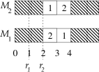
Figure 1: Non-delay and vertical order properties

Remark 1

When preemption is allowed, non-delay schedules are dominant for regular criteria since it is always possible to move a piece of a job to an earlier idle time interval without increasing the objective function. Moreover, vertically ordered schedules are also dominant since the completion times of the jobs remain the same if the pieces of jobs scheduled in the same time interval are reassigned to processors in order to respect the vertical order.

We assume without loss of generality that $r_{1}\leq r_{2}\leq\dots\leq r_{n}$ for the remainder of the paper. Now, let us characterize the structure:

Definition 1

A schedule is said to be Permutation Flow Shop-like ($PFS-like$) if

1. it is vertically ordered,

2. no machine processes more than one piece of each job,

3. the scheduling order on the different machines is the same.

An example of $PFS-like$ schedule is given in Figure 2.

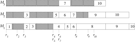
Figure 2: A $PFS-like$ schedule for $P|pmtn,r_{j}|f$

It is interesting to mention that for the problem $P|pmtn,r_{j},p_{j}=p|\sum C_{j}$, Baptiste et al. (2007) show that a similar structure is dominant. This result is very specific since it deals with equal processing times and the considered objective function is the total completion time. In this paper, we prove the existence of such a structure for more general problems.

Now, we express our central result:

Theorem 1

If $P|pmtn,r_{j}|f$ has a solution $S$ with completion times $C_{1}\leq C_{2}\leq\dots\leq C_{n}$, there exists a non-delay $PFS-like$ solution $S^{\prime}$ such that $C_{1}^{\prime}\leq C_{2}^{\prime}\leq\dots\leq C_{n}^{\prime}$ and $C_{j}^{\prime}\leq C_{j}$ for $1\leq j\leq n$.

Proof. By Remark 1, we assume without loss of generality that $S$ is a non-delay schedule which is vertically ordered. Let us define the following two properties:

$A(j)$:

If $i$ and $i^{\prime}$ are two jobs such that $1\leq i\leq j$ and $i<i^{\prime}$ no machine processes a piece of job $i^{\prime}$ before a piece of job $i$.

$B(j)$:

“No machine processes more than one piece of job $i$, for $1\leq i\leq j$.

If $A(n)$ and $B(n)$ are true, $S$ is a non-delay $PFS-like$ solution. Otherwise, we prove by induction on the job number that $S$ can be transformed into a non-delay and vertically ordered schedule $S^{\prime}$ such that $A(n)$ and $B(n)$ are true.

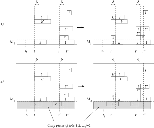
Figure 3: The basic transformation used in Theorem 1.

Base step.

By Remark 1, vertically-ordered schedules are dominant and hence each piece of job $1$ is processed by machine $M_{1}$.

If $A(1)$ is true then $B(1)$ must be true: otherwise $M_{1}$ processes two pieces of job $1$ that are separated by an idle time interval, which contradicts the non-delay assumption.

So, suppose $A(1)$ is false and consider the smallest $t$ such that a job $k>1$ starts on $M_{1}$ at $t$ before a piece of job $1$. Let $t^{\prime}$ be the starting time of this piece of job $1$ (see case 1 of Figure 3). The non-delay property implies that all machines are busy during time interval $[t,t^{\prime}[$. Since $|J(t)|=m$, and $|J(t^{\prime})-\{1\}|\leq m-1$, there is a piece of a job $l$ processed at time $t$ that is not processed at time $t^{\prime}$. Moreover, since $C_{1}\leq C_{l}$ (by definition of $S$), there is also another piece of job $l$ that starts at time $t^{\prime\prime}>t^{\prime}$. Let $\delta=\min(t^{\prime\prime}-t^{\prime},\min_{i\in J(t)}\{C(i,t)-t\},\min_{i\in J(t^{\prime})}\{C(i,t^{\prime})-t^{\prime}\})$. We exchange the piece of job $l$ processed during time interval $[t,t+\delta[$ with the piece of job $1$ processed during time interval $[t^{\prime},t^{\prime}+\delta[$. Finally, we reassign pieces of jobs processed during time interval $[t,t+\delta[$ and pieces of jobs processed during time interval $[t^{\prime},t^{\prime}+\delta[$ respectively, so that the schedule remains vertically ordered. Only the completion time of job $1$ may decrease and the new schedule is still a non-delay one. Moreover, there is now a piece of job $1$ processed on machine $M_{1}$ during time interval $[t,t+\delta[$. If $t>r_{1}$, the non-delay property of $S$ and the definition of $t$ imply that there is a piece of job $1$ processed during time interval $[r_{1},t[$, so there is now one single piece of job $1$ processed during time interval $[r_{1},t+\delta[$ by machine $M_{1}$. If $A(1)$ is true, so is $B(1)$. Otherwise, we consider again the smallest $\tau$ such that a job $k>1$ starts on $M_{1}$ at $\tau$ before a piece of job $1$: since $\tau\geq t+\delta$ and $\delta>0$ we have $\tau>t$. Therefore, by repeating this procedure, either we do not find such a $\tau$ or we reach the end of the schedule: in both cases $A(1)$ becomes true, so does $B(1)$.

Induction step.

Now, suppose there is a non-delay and vertically ordered schedule such that $A(j-1)$ and $B(j-1)$ are true for $j\geq 2$, and assume that at least one of the properties $A(j)$ and $B(j)$ is false.

If $A(j)$ is true then $B(j)$ must be true. Indeed, suppose for the sake of contradiction that $B(j)$ is false. In this case, there is one machine $M_{q}$ which processes two pieces of job $j$. Let $t$ and $t^{\prime}>t$ be their completion and starting times, respectively. If the machine is idle during time interval $[t,t^{\prime}[$, we get a contradiction. Indeed, if $q=1$ the non-delay assumption is not verified. If $q>1$, let $i$ be a job processed at time $t^{\prime}$ on a machine $M_{p}$, with $p<q$: since the schedule is vertically ordered, we have $i<j$, and since $A(j-1)$ is true, no piece of job $j$ can be processed by machine $M_{p}$ during time interval $[r_{1},t^{\prime}[$. Hence, no piece of job $j$ is processed by machines $M_{1},M_{2},\ldots,M_{q-1}$ during time interval $[t,t^{\prime}[$, and the piece of job $j$ starting at time $t^{\prime}$ can start earlier at time $t$, which contradicts the non-delay assumption.

So, suppose $A(j)$ is false, and let us consider the smallest value $t$ such that a piece of a job $k>j$ starts at time $t$, and a piece of job $j$ starts at time $t^{\prime}>t$, on a machine $M_{q}$ (see case 2 of Figure 3). Since $k>j$ and the schedule is vertically ordered, no piece of job $j$ can be processed by machines $M_{q+1},M_{q+2},\ldots,M_{m}$ during time interval $[t,C(k,t)[$. If $q=1$, no piece of job $j$ can be processed during this time interval. Else, let $i$ and $i^{\prime}$ be the jobs processed respectively at time $t$ and $t^{\prime}$ by machine $M_{q-1}$. Since the schedule is vertically ordered, we have $i^{\prime}<j$, and since $A(j-1)$ is true we have $i\leq i^{\prime}$, so we get $i<j$. Consequently, no piece of job $j$ can be processed by machines $M_{1},M_{2},\ldots,M_{q-1}$ during time interval $[t,C(k,t)[$.

Since it is a non-delay schedule and $r_{j}\leq r_{k}\leq t$, all machines are busy during time interval $[t,t^{\prime}[$: therefore there is a piece of a job $l>k$ processed at time $t$ that is not processed at time $t^{\prime}$. Since $C_{j}\leq C_{l}$ (by definition of $S$), there is also another piece of job $l$ that starts at time $t^{\prime\prime}>t^{\prime}$. Let $\delta=\min(t^{\prime\prime}-t^{\prime},\min_{i\in J(t)}\{C(i,t)-t\},\min_{i\in J(t^{\prime})}\{C(i,t^{\prime})-t^{\prime}\})$. We exchange the piece of job $l$ processed during time interval $[t,t+\delta[$ with the piece of job $j$ processed during time interval $[t^{\prime},t^{\prime}+\delta[$. Finally, we reassign pieces of jobs processed during time interval $[t,t+\delta[$ and pieces of jobs processed during time interval $[t^{\prime},t^{\prime}+\delta[$ respectively, so that the schedule remains vertically ordered.

Again, only the completion time of job $j$ may decrease, and we still have a non-delay schedule. Moreover there is a piece of job $j$ processed on machine $M_{q}$ during time interval $[t,t+\delta[$. If there is also a piece of job $j$ processed by $M_{q}$ before time $t$, it must end at time $t$ (by definition of $t$ and because of the non-delay assumption). Hence, machine $M_{q}$ processes no piece of a job $k>j$ and only one single piece of job $j$ during time interval $[0,t+\delta[$. Since $\delta>0$, we can repeat the procedure, as in the ”base step”, and get a schedule with $A(j)$ and $B(j)$ being true. $\blacksquare$

Remark 2

For problems without release date, i.e. of the form $P|pmtn|f$, non-delay $PFS-like$ schedules are dominant since, by renumbering the jobs, there always exists an optimal solution such that $C_{1}^{*}\leq C_{2}^{*}\leq\dots\leq C_{n}^{*}$.

This theorem gives a very precise structure on an optimal solution for problems of the form $P|pmtn,r_{j}|f$ for which there exists an optimal solution $S^{*}$ such that $r_{j}<r_{k}\implies C_{j}^{*}\leq C_{k}^{*}$. Moreover, this structure is very interesting combined with a dominant order for the jobs’ completion times, because it can lead to the time-polynomiality of a large class of problems. Indeed, the linear programming approach proposed by Baptiste et al. (2007) for problem $P|pmtn,r_{j},p_{j}=p|\sum C_{j}$ can be extended to regular criteria which are separable piecewise continuous linear, such as $\sum w_{j}T_{j}$ for example.

Let us modify their linear program. The value $p$ is replaced with $p_{j}$ in the job processing time constraints, and the objective function is replaced with a regular criterion $f$ which is a separable piecewise continuous linear function. Properties of $f$ ensure that it can be handled by a linear program (see for instance Dantzig and Thapa (1997)). We then get:

minimize $$f(C_{1},C_{2},\ldots,C_{n})$$

subject to

$$\sum_{l=1}^{m}p_{j}^{l} =p_{j} \forall j=1,\ldots,n$$ (1)

$$t_{j}^{l+1}+p_{j}^{l+1} \leq t_{j}^{l} \forall j=1,\ldots,n,\forall l=1,\ldots,m-1$$ (2)

$$t_{j}^{l}+p_{j}^{l} \leq t_{j+1}^{l} \forall j=1,\ldots,n-1,\forall l=1,\ldots,m-1$$ (3)

$$t_{j}^{m} \geq r_{j} \forall j=1,\ldots,n$$ (4)

$$t_{j}^{1}+p_{j}^{1} =C_{j} \forall j=1,\ldots,n$$ (5)

$$p_{j}^{l},t_{j}^{l} \geq 0 \forall j=1,\ldots,n,\forall l=1,\ldots,m$$ (6)

$$C_{j} \geq 0 \forall j=1,\ldots,n$$ (7)

The ${\cal O}(nm)$ variables $t_{j}^{l},p_{j}^{l}$, and $C_{j}$ are defined respectively as the starting time of job $j$ on machine $M_{l}$, the processing time of job $j$ on machine $M_{l}$, and the completion time of job $j$. Equalities (1) guarantee the processing time of each job, whereas inequalities (2) ensure that a job is first processed on the different machines in the order $M_{m}$, $M_{m-1}$, $\dots$, $M_{1}$. Inequalities (3) ensure that jobs are scheduled on each machine following order $1,2,\ldots,n$.

Theorem 2

The problem $P|pmtn,r_{j}|f$ can be solved in polynomial time if $f$ is a separable piecewise continuous linear function computable in polynomial time and if there exists an optimal solution such that $C_{1}^{*}\leq C_{2}^{*}\leq\dots\leq C_{n}^{*}$.

Proof. We use Theorem 1 with the idea of the proof in  Baptiste et al. (2007). Theorem 1 implies that there exists an optimal non-delay $PFS-like$ solution such that the order of the jobs on each machine is $1,2,\ldots,n$. If we denote by $z^{*}$ its value, and by $w^{*}$ the minimum value of a $PFS-like$ solution which verifies order $1,2,\ldots,n$ for the jobs, we have $z^{*}\leq w^{*}$. Now, observe that any solution of the linear program defines a $PFS-like$ schedule. Hence, if $f^{*}$ is the value of an optimal solution of the linear program, we get $f^{*}\geq w^{*}$, that is $f^{*}\geq z^{*}$. However, in a $PFS-like$ schedule a job $j$ may have a completion time less than $C_{j}$ because there may be no piece of $j$ on machine $M_{1}$. So, let us show that the optimal non-delay $PFS-like$ solution (denoted by $\sigma$) verifies the constraints of the linear program. Suppose there is a job $j$ in $\sigma$ that completes at time $C^{\sigma}_{j}$ and whose last piece is processed by machines $M_{q}$ with $q>1$. By Theorem 1 we know that there is no job $i<j$ such that $C^{\sigma}_{i}>C^{\sigma}_{j}$, and also that $\sigma$ is vertically ordered, so no job $i>j$ is scheduled by processors $M_{1},M_{2},\ldots,M_{q}$ before time $C^{\sigma}_{j}$: therefore, we can define a solution of the linear program such that $p^{l}_{j}=0$ for $1\leq l<q$, that is such that $C_{j}=C^{\sigma}_{j}$. By applying this procedure to any job $j$ whose last piece is not processed by machine $M_{1}$, we get a solution of the linear program of value $z^{*}$, which implies $z^{*}\geq f^{*}$. From $z^{*}\leq f^{*}$ we deduce that $f^{*}=z^{*}$: the optimal solution of the linear program is also an optimal solution of the problem $P|pmtn,r_{j}|f$ . $\blacksquare$

Note that a more general LP formulation is proposed in Kravchenko and Werner (2012), since it is dedicated to solve the problem $Q|r_{j},pmtn,D_{j},C_{1}\leq\dots\leq C_{n}|F$, where $C_{1}\leq\dots\leq C_{n}$ means that we are only looking for an optimal schedule among the class of schedules for which $C_{1}\leq\dots\leq C_{n}$ holds. Nevertheless, notice that the formulation introduced here is interesting for two reasons: first, this LP formulation involves only $O(nm)$ variables and $O(nm)$ constraints, whereas the one proposed in Kravchenko and Werner (2012) uses $O(n^{3}m)$ variables and constraints. Secondly, the approach provided in Kravchenko and Werner (2012) does not allow us to use the $PFS-like$ structure proposed in this paper.

The next section is dedicated to finding subproblems of $P|pmtn,r_{j}|f$ for which a total order on jobs’ completion times can be obtained, in order to conclude that they are solvable in polynomial time.

3 Ordering the jobs’ completion times

Extending notations on the agreeability introduced in Tian et al. (2009), in the $\beta$-field, we write $(r_{j}^{+},p_{j}^{+})$ if $r_{j}$’s and $p_{j}$’s are in the same order, i.e. $p_{1}\leq p_{2}\leq\dots\leq p_{n}$. Note that, for a problem with equal processing times, or without release dates, this condition is always fulfilled. This notation can also be used for more than two inputs; for example, $(r_{j}^{+},p_{j}^{+},d_{j}^{+},w_{j}^{-})$ means that $r_{j}$’s, $p_{j}$’s and $d_{j}$’s are in an increasing order whereas $w_{j}$’s are decreasing.

Under some specific conditions on the objective functions and the input data, it is possible to know the order of the jobs’ completion times in an optimal solution:

Theorem 3

The following problems are solvable in polynomial time:

1. $P|pmtn,(r_{j}^{+},p_{j}^{+})|\sum f_{j}$, when $f_{j}$’s are regular functions and $f_{j}-f_{k}$ is non-decreasing if $j<k$.

2. $P|pmtn,(r_{j}^{+},p_{j}^{+})|\max f_{j}$, when $f_{j}$’s are regular functions and $f_{j}-f_{k}$ is non-negative if $j<k$.

3. $P|pmtn,(r_{j}^{+},p_{j}^{+},w_{j}^{-}),d_{j}=d|\sum w_{j}U_{j}$.

Proof. We first show that there exists an optimal schedule such that $C_{1}^{*}\leq C_{2}^{*}\leq\dots\leq C_{n}^{*}$. Let $S$ be an optimal schedule. For the sake of contradiction, assume that there exist two jobs $j<k$, such that $r_{j}\leq r_{k}$, $p_{j}\leq p_{k}$ and $C_{j}>C_{k}$, and let us prove that we can find another optimal schedule $S^{\prime}$ such that $C_{j}^{\prime}\leq C_{k}^{\prime}$. This exchange argument is illustrated with Figure 4.

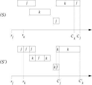
Figure 4: An optimal solution and the corresponding optimal solution after the exchange.

The schedule $S^{\prime}$ is constructed in the following manner: all the pieces of jobs but $j$ and $k$ remain exactly at the same position. All pieces of job $j$ processed before $r_{k}$ stay at the same place, and on any time interval where jobs $j$ and $k$ are both processed in $S$, we schedule them in the same manner in $S^{\prime}$. For the remaining available slots, starting from time $r_{k}$, we schedule the remaining part of job $j$ and then the one of $k$. By construction, we ensure that no overlap exists in $S^{\prime}$ by scheduling jobs $j$ and $k$ in $S^{\prime}$ when $j$ and $k$ are simultaneously processed in $S$. Using the fact that $p_{j}\leq p_{k}$, the completions times of $j$ and $k$ are $C_{j}^{\prime}\leq C_{k}$ and $C_{k}^{\prime}=C_{j}$.

Now, let us consider the three cases:

1. Since $f_{j}-f_{k}$ is a non-decreasing function, by considering time points $C_{j}$ and $C_{k}$, we can write $(f_{j}-f_{k})(C_{j})\geq(f_{j}-f_{k})(C_{k})$, which means that $f_{j}(C_{k})+f_{k}(C_{j})\leq f_{j}(C_{j})+f_{k}(C_{k})$.

2. We have $\max(f_{j}(C_{j}^{\prime}),f_{k}(C_{k}^{\prime}))\leq\max(f_{j}(C_{j}),f_{k}(C_{j}))$ and, using the fact that $f_{j}-f_{k}$ is a non-negative function, we can write $\max(f_{j}(C_{j}),f_{k}(C_{j}))=f_{j}(C_{j})\leq\max(f_{j}(C_{j}),f_{k}(C_{k}))$.

3. We have to consider three cases according to the value of $d$; if $d\geq C_{j}$, we have $U^{\prime}_{j}=U_{j}=0$ and $U^{\prime}_{k}=U_{k}=0$. If $C_{k}>d$ then $U^{\prime}_{j}\leq U_{j}=1$ and $U^{\prime}_{k}=U_{k}=1$. In both cases we get $w_{j}U^{\prime}_{j}+w_{k}U^{\prime}_{k}\leq w_{j}U_{j}+w_{k}U_{k}$ Finally, if $C_{j}>d\geq C_{k}$ then $U^{\prime}_{j}=U_{k}=0$ and $U^{\prime}_{k}=U_{j}=1$, so we get $w_{j}U^{\prime}_{j}+w_{k}U^{\prime}_{k}=w_{k}\leq w_{j}=w_{j}U_{j}+w_{k}U_{k}$ .

Hence, $S^{\prime}$ is also optimal in all cases, and there exists an optimal schedule such that $C_{1}^{*}\leq C_{2}^{*}\leq\dots\leq C_{n}^{*}$. Therefore, problems of cases 1 and 2 are solvable in polynomial time by Theorem 2. For case 3, Theorem 2 cannot be used because $f_{j}$’s functions are not continuous. However, we only need to find the first job $k$ that cannot be on time, since jobs $l>k$ will be also late, by Theorem 1. This can be done by testing the feasibility of successive modified versions of the linear program of Theorem 2: for $k=1,2,\ldots,n$, only on-time jobs $1\leq j\leq k$ are considered, and constraints $t^{1}_{j}+p^{1}_{j}\leq d$, for $1\leq j\leq k$, are added. $\blacksquare$

These results are used in the next section to derive time-polynomially solvable problems according to different classical criteria.

4 Consequences on classical criteria problems

Figure 5 shows the new complexity hierarchy of parallel identical machine scheduling problems with preemption and release dates for criteria based on the $\sum w_{j}T_{j}$ . Previously minimal $\cal NP$-hard and maximal time-polynomially solvable problems are included with their references, and shaded results are the ones proved with the unified approach proposed in this paper.

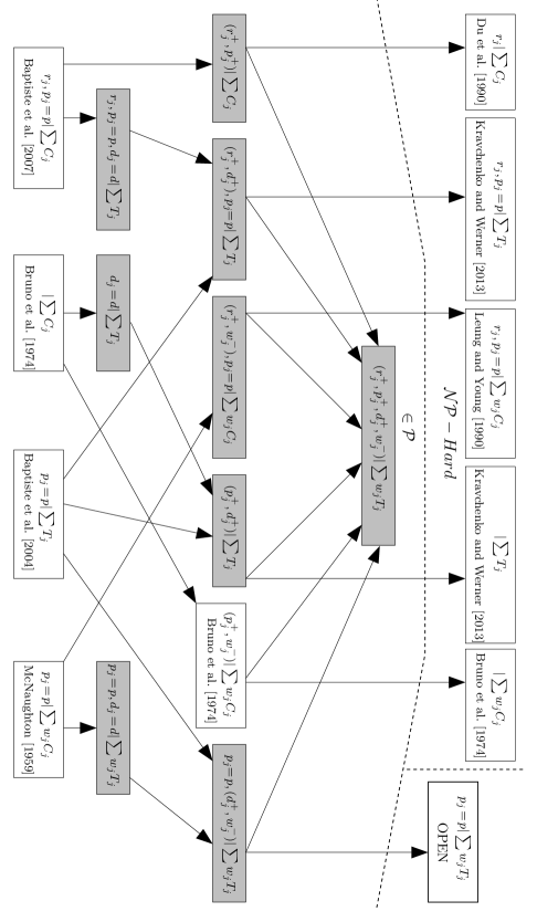
Figure 5: Classification of scheduling problems of type $P|pmtn,r_{j}|\sum w_{j}T_{j}$. “$P|pmtn,$” is omitted. An arc means “is a subproblem of”. In gray, main results provided in this paper with a unified approach.

For the four types of input data $r_{j},p_{j},d_{j}$ and $w_{j}$ there exist many agreeable combinations. In order to present a synthetic view, we consider cases where some of the data are constant, i.e. $r_{j}=0$, $p_{j}=p$, $d_{j}\in\{0,d\}$ or $w_{j}=1$. Thus, we distinguish the two following cases:

a) Three types of data have constant values: all the problems are solvable in polynomial time, by Theorem 3. More precisely, if $d_{j}=0$ or if $d_{j}$ is not fixed, these results were already known. It is interesting to notice that some of them were proved more than 30 years ago, whereas the others are very recent (Baptiste et al. (2004) and Baptiste et al. (2007)). We extend these results and prove the time-polynomiality of the six problems we get by the combinations of parameters and criteria when $dj=d$, which is known in the literature as the ’common due date’ case.

b) Two types of data have constant values: if the remaining data verify the condition of Theorem 3, then the corresponding problem is in $\cal P$  we hence provide a polynomial-time algorithm for different problems with agreeable conditions, for which very few results were known. Otherwise, i.e. if the remaining data do not necessary satisfy the condition of Theorem 3, using a literature review, we observe that the problem is either $\cal NP$-hard or open. For flow-time or tardiness criteria, all problems are $\cal NP$-hard, except $P|pmtn,p_{j}=p|\sum w_{j}T_{j}$: that is why we conjecture it is $\cal NP$-Hard.

Our approach also defines new problems with common due dates for which complexity issues are interesting for criteria related to weighted total number of late jobs. When we have to deal with common due dates and a criterion based on $\sum w_{j}U_{j}$, it is possible to look at the reverse problem and hence provide directly complexity results. For example, $P|r_{j},d_{j}=d,pmtn|\sum U_{j}$ is equivalent by symetry to $P|pmtn|\sum U_{j}$ and is hence NP-Hard. In the same way, problem $P|pmtn,r_{j},p_{j}=p,d_{j}=d|\sum U_{j}$ is equivalent to $P|pmtn,p_{j}=p|\sum U_{j}$, for which a polynomial time algorithm was given in Baptiste et al. (2004). Our approach leads to a slightly more general result since we show that $P|pmtn,(r_{j}^{+},p_{j}^{+},w_{j}^{-}),d_{j}=d|\sum w_{j}U_{j}$ is solvable in polynomial time.

One can also note that our approach does not perform well for a criterion of type $f=\max f_{j}$. Indeed, we can only prove that $P|pmtn|C_{max}$ and $P|pmtn,p_{j}=p|L_{max}$ are in $\cal P$, whereas it was independently proved in Lawler and Labetoulle (1978) and Slowinski (1981) that $R|pmtn,r_{j}|L_{max}$ can be solved in polynomial time.

5 Conclusion

In this paper we proved that there exists a type of schedules (named $PFS-like$) which is dominant for problem $P|pmtn,r_{j}|f$ if there exists an optimal solution with completion times scheduled in the same order as the release dates, or if there is no release date. By interchange arguments, we proved that, for a large subclass of these problems, it is possible to order the optimal completion time of all jobs. Using these two results, we showed that problems satisfying the condition of Theorem 3 are polynomially solvable. In particular, we proved the polynomiality of different problems having agreeable data and/or a common due date $d_{j}=d$.

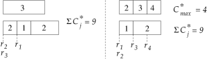
Figure 6: Finding a better characterization of $PFS-like$ schedules

An interesting question consists in finding a less restrictive condition for the existence of $PFS-like$ schedules. Indeed, on the one hand, $PFS-like$ schedules are not dominant if condition $(r_{j}^{+},p_{j}^{+})$ does not hold (see left chart of Figure 6) but, on the other hand, there exist $PFS-like$ schedules that are optimal, even if the condition $(r_{j}^{+},p_{j}^{+})$ is not verified (right chart of Figure 6). Hence, we should seek for a better characterization of the conditions implying the existence of $PFS-like$ schedules.

Another research avenue lies in using the $PFS-like$ structure in $\cal NP$-Hard problems to derive approximation algorithms or to improve resolution methods; indeed, the existence of $PFS-like$ schedules drastically reduces the combinatoric of problems since, whatever the number of machines, there are at most $n!$ orders to test.

Finally, polynomial-time cases for problem $P|pmtn,r_{j}|f$ that were already solved in the literature are also polynomially solvable when we generalize to the uniform machine case $Q|pmtn,r_{j}|f$, leading to the natural following question: is the $PFS-like$ structure also dominant for some problems in case of uniform machines?

References

- Baptiste et al. (2007) Baptiste, P., Brucker, P., Chrobak, M., Dürr, C., Kravchenko, S., Sourd, F., 2007. The complexity of mean flow time scheduling problems with release times. Journal of Scheduling 10, 139–146.
- Baptiste et al. (2004) Baptiste, P., Brucker, P., Knust, S., Timkovsky, V., 2004. Ten notes on equal-execution-time scheduling. 4OR 2, 111–127.
- Blazewicz et al. (1976) Blazewicz, J., Cellary, W., Slowinski, R., Weglarz, J., 1976. Deterministyczne problemy szeregowaia zadan na równoleglych procesorach, Czesc I: zbiory zadan niezaleznych (Deterministic problem of scheduling tasks on parallel processors. Part I: set of independent tasks). Podstawy Sterowania 6, 155–178.
- Blazewicz et al. (1991) Blazewicz, J., Dror, M., Weglarz, J., 1991. Mathematical programming formulations for machine scheduling: a survey. European Journal of Operational Research 51 (3), 283–300.
-
Brucker and Knust (2013)
Brucker, P., Knust, S., 2013. Complexity results for scheduling problems.
URL http://www.informatik.uni-osnabrueck.de/knust/class - Brucker and Kravchenko (2006) Brucker, P., Kravchenko, S., 2006. Scheduling equal processing time jobs to minimize the weighted number of late jobs. Journal of Mathematical Modelling and Algorithms 5, 143–165.
- Bruno et al. (1974) Bruno, J., Coffman, Jr., E. G., Sethi, R., 1974. Scheduling independent tasks to reduce mean finishing time. Commun. ACM 17, 382–387.
- Dantzig and Thapa (1997) Dantzig, G., Thapa, M., 1997. Linear Programming: 1: Introduction. Springer.
- Du et al. (1990) Du, J., Leung, J.-T., Young, G., 1990. Minimizing mean flow time with release time constraint. Theoretical Comput. Sci. 75, 347–355.
-
Dürr (2013)
Dürr, C., 2013. The scheduling zoo.
URL http://www-desir.lip6.fr/~durrc/query - Giffler and Thompson (1960) Giffler, B., Thompson, G. T., 1960. Algorithms for solving production scheduling problems. Operations Research 8, 487–503.
- Graham et al. (1989) Graham, R., Lawler, E., Lenstra, J., Rinnooy Kan, A., 1989. Optimization and approximation in deterministic sequencing and scheduling: a survey. Annals of Discrete Mathematics 5, 287–326.
- Kravchenko (2000) Kravchenko, S., 2000. On the complexity of minimizing the number of late jobs in unit time open shop. Discrete Applied Mathematics (DAM) 100, 127–132.
- Kravchenko and Werner (2011) Kravchenko, S., Werner, F., 2011. Parallel machine problems with equal processing times: a survey. Journal of Scheduling 14, 435–444.
- Kravchenko and Werner (2012) Kravchenko, S., Werner, F., 2012. Linear Programming - New Frontiers in Theory and Applications. Nova Publishers, Ch. Minimizing a regular function on uniform machines with ordered completion times, pp. 159–172.
-
Kravchenko and Werner (2013)
Kravchenko, S., Werner, F., 2013. Erratum to: Minimizing total tardiness on
parallel machines with preemptions. Journal of Scheduling, 1–3.
URL http://dx.doi.org/10.1007/s10951-013-0313-5 - Lawler (1983) Lawler, E., 1983. Recent results in the theory of machine scheduling. In: Bachem, A., Groetschel, M., Korte, B. (Eds.), Mathematical programming: the state of the art (Bonn, 1982). Springer, Berlin, pp. 202–234.
- Lawler and Labetoulle (1978) Lawler, E., Labetoulle, J., 1978. On Preemptive Scheduling of Unrelated Parallel Processors by Linear Programming. Journal of the ACM 25, 612–619.
- Leung and Young (1990) Leung, J.-T., Young, G., 1990. Preemptive scheduling to minimize mean weighted flow time. Information Processing Letters 34, 47–50.
- McNaughton (1959) McNaughton, R., 1959. Scheduling with deadlines and loss functions. Management Science 6, 1–12.
- Slowinski (1981) Slowinski, R., 1981. L’ordonnancement des tâches préemptives sur les processeurs indépendants en présence de ressources supplémentaires (Scheduling preemptive tasks on unrelated processors with additional resources). RAIRO Informatique 15, 155–166.
- Tian et al. (2009) Tian, Z., Ng, C., Cheng, T., 2009. Preemptive scheduling of jobs with agreeable due dates on a single machine to minimize total tardiness. Operations Research Letters (ORL) 37, 368–374.