Application of Quadrature Methods for Re-Weighting in Lattice QCD

Abstract:

Re-weighting is a useful tool that has been employed in Lattice QCD in different contexts including, tuning the strange quark mass, approaching the light quark mass regime, and simulating electromagnetic fields on top of QCD gauge configurations. In case of re-weighting the sea quark mass, the re-weighting factor is given by the ratio of the determinants of two Dirac operators $D_{a}$ and $D_{b}$. A popular approach for computing this ratio is to use a pseudofermion representation of the determinant of the composite operator $\Omega=D_{a}(D_{b}^{\dagger}D_{b})^{-1}D_{a}^{\dagger}$. Here, we study using quadrature methods together with noise vectors to compute the ratio of determinants. We show that, with quadrature methods each determinant can be computed separately using the operators $\Omega_{a}=D_{a}^{\dagger}D_{a}$ and $\Omega_{b}=D_{b}^{\dagger}D_{b}$. We also discuss using bootstrap re-sampling to remove the bias from the determinant estimator.

1 Introduction

Re-weighting is a useful tool that has been applied recently in lattice QCD simulations in different contexts. The main idea is that the expectation value of an observable $O$ with respect to an action $S_{b}$ can be written in terms of expectation values with respect to another action $S_{a}$ as follows:

$$\langle O\rangle_{b} := \frac{1}{Z_{b}}\int{\cal{D}}U\ O[U]\ e^{-S_{b}}$$ (1)

$$= \frac{Z_{a}}{Z_{b}}\frac{1}{Z_{a}}\int{\cal{D}}U\ O[U]\ w[U]e^{-S_{a}}$$

$$= \frac{\langle O\ w\rangle_{a}}{\langle w\rangle_{a}},$$

where $Z_{a}$ and $Z_{b}$ are the corresponding partition functions, $U$ is the gauge configuration and $w[U]$ is called the reweighting factor corresponding to the gauge configuration $U$ and is defined by $w[U]:=\frac{e^{-S_{b}[U]}}{e^{-S_{a}[U]}}$. The labels ”a” and ”b” refers to a particular choice of the action parameters such as the sea quark mass. Equation 1 is exact. However, when using importance sampling and for a finite set of gauge configurations, reweighting could be biased. Because of this bias, reweighting is only reliable when there is a small change between the actions $S_{a}$ and $S_{b}$, and the reweighting factors normalized by the ensemble mean are $O(1)$.

An important application of reweighting methods is mass reweighting in which observables corresponding to a sea quark mass $m_{b}$ are computed using configurations generated with a sea quark mass $m_{a}$. In this case the reweighting factor is given by

$$w[U]=\frac{\det[(D(U;m_{b})^{\dagger}D(U;m_{b}))^{\frac{n_{f}}{2}}]}{\det[(D(U;m_{a})^{\dagger}D(U;m_{a}))^{\frac{n_{f}}{2}}]},$$ (2)

where $D(U;m)$ is the Dirac operator for gauge configuration $U$ and bare quark mass $m$ and $n_{f}$ is the number of degenerate flavors being re-weighted. Applications of mass reweighting include tuning the strange quark mass in dynamical Domain-Wall simulations to its physical value [3], computing the strange Nucleon sigma term using the Feynman-Hellman theorem [4], simulating the $\epsilon$ regime [2], and tuning to the physical point in 2+1 simulations of the PACS-CS collaboration [5].

A common approach for computing the ratio of determinants is using pseudofermions. This has been the main technique used for mass reweighting [2, 3, 5]. In this approach, the relation

$$\frac{1}{\det(\Omega)}=\frac{\int{\cal{D}}\xi^{\dagger}{\cal{D}}\xi\ e^{-\xi^{\dagger}\Omega\xi}}{\int{\cal{D}}\xi^{\dagger}{\cal{D}}\xi\ e^{-\xi^{\dagger}\xi}}$$ (3)

is used to compute the determinant of a matrix $\Omega$. The right-hand side of Equation (3) is computed stochastically as an average over random gaussian fields $\xi$ generated with the distribution $e^{-\xi^{\dagger}\xi}$ as

$$<\frac{1}{\det(\Omega)}>_{\xi}=<e^{-\xi^{\dagger}(\Omega-1)\xi}>_{\xi},$$ (4)

where the notation $<g>_{\xi}$ means expectation value of $g$ over $\xi$. For a reliable estimate of $\det(\Omega)$ using Equation (4), $\Omega$ need to be close to the identity matrix. For $n_{f}$ degenerate flavors,

$$\Omega=[D_{a}(D_{b}^{\dagger}D_{b})^{-1}D_{a}^{\dagger}]^{\frac{n_{f}}{2}}.$$ (5)

For small changes in the fermion action, $\Omega$ will be close to the identity matrix. In addition, it is possible to improve the estimation of $\det(\Omega)$ by dividing the change of the Dirac operator into smaller steps and writing the ratio of determinants as a product of $k+1$ factors

$$\frac{\det(D_{a})}{\det(D_{b})}=\frac{\det(D_{a})}{\det(D_{1})}\ \frac{\det(D_{1})}{\det(D_{2})}\ \dots\frac{\det(D_{k-1})}{\det(D_{k})}\ \frac{\det(D_{k})}{\det(D_{b})},$$ (6)

such that the ratio of determinants in each factor is close to one. The pseudofermion approach has the advantage of giving directly an unbiased estimator of the ratio of determinants. It however requires the solution of a linear system for each $\xi$. Another difficulty with the pseudofermion approach is that, for a single flavor reweighting, it requires using a rational approximation for the square root of a matrix which in turn requires a multi-shift solver. We study here an alternative way of computing the ratio of determinants based on the relation $\det(\Omega)=e^{\rm{trace}[\log(\Omega)]}$. In our approach, the trace of $\log(\Omega)$ is evaluated using noise methods and the matrix elements of $\log(\Omega)$ between noise vectors are computed using Gauss quadratures [6]. This approach has been proposed in the context of generating dynamical electromagnetic field configurations on top of existing QCD configurations [7]. In this paper, we elaborate on using this approach also for mass reweighting. In addition, we show that the need to solve a linear system for each noise vector can be avoided by computing the determinant of each Dirac operator separately and then take the ratio. This leads to a faster evaluation of the reweighting factor than what is usually used in the literature. Another advantage of using the relation $\det(\Omega)=e^{\rm{trace}[\log(\Omega)]}$ is that including a fractional power is trivial since

$$\det(\Gamma^{\alpha})=e^{\rm{trace}[\log(\Gamma^{\alpha})]}=e^{\alpha\rm{trace}[\log(\Gamma)]}.$$ (7)

Finally, variance reduction techniques such as breaking the ratio of determinants into factors and dilution can be used. It is noted that dilution couldn’t be used with pseudofermions.

2 Quadrature and Noise approach

Let $z$ be a vector whose elements are random variables satisfying

$$<z_{i}z_{j}>=<z_{i}^{*}z_{j}>=\delta_{ij}.$$ (8)

Such vectors are called noise vectors. For a matrix $H$, we have

$$\langle z^{\dagger}Hz\rangle_{noise} = trace[H],$$

$$var(z^{\dagger}Hz)_{noise} = \sum_{i\neq j}|H_{ij}|^{2}+H_{ij}H_{ji}^{*},$$ (9)

where $\langle\dots\rangle_{noise}$ and $var(\dots)_{noise}$ means the expectation value and variance over the set of noise vectors. For a positive definite Hermitian matrix $H$, the element $z^{\dagger}Hz$ can be written as a Riemann-Stieltjes integral which can then be computed using Gauss quadrature methods (see [6] for more details). For computing the ratio of determinants, one could define $\Omega=D_{a}(D_{b}^{\dagger}D_{b})^{-1}D_{a}^{\dagger}$ and take $H:=log(\Omega)$, then use Equation [7]. In this case, $\Omega$ is close to the identity, however, each application of $\Omega$ to a vector requires the solution of a linear system which is expensive. We call this the standard method. Alternatively, one could compute each determinant separately using the operators $\Omega_{a}=D_{a}^{\dagger}D_{a}$ and $\Omega_{b}=D_{b}^{\dagger}D_{b}$. Although these operators are not close to the identity, they don’t involve the inverse making this approach potentially faster. We call this the difference method.

Our tests are done using Clover fermions. In this case it is advantageous to use use even-odd preconditioning. The Dirac operator is written in the form

$$D=\left(\begin{array}[]{cc}D_{ee}&D_{eo}\\ D_{oe}&D_{oo}\end{array}\right)=\left(\begin{array}[]{cc}1&0\\ D_{oe}D^{-1}_{ee}&1\end{array}\right)\left(\begin{array}[]{cc}G&0\\ 0&Q\\ \end{array}\right)\left(\begin{array}[]{cc}1&D^{-1}_{ee}D_{eo}\\ 0&1\\ \end{array}\right),$$ (10)

where $G=D_{ee}$ and $Q=D_{oo}-D_{oe}D^{-1}_{ee}D_{eo}$ is the Schur complement. The determinant of the Dirac operator is then given by $\det\left(D\right)=\det\left(G\right)\det\left(Q\right)$. For this decomposition, $\det\left(G\right)$ can be computed exactly and cheaply while $\det\left(Q\right)$ is estimated using noisy estimators.

Noisy estimators give an unbiased estimate for the trace of the logarithm. In order to get an unbiased estimate of the determinant by taking the exponential of the trace of the logarithm, additional techniques are needed. There are two possible ways to obtain such unbiased estimator. The first method is using a resampling technique such as bootstrap (or jackknife). The second method, which is applicable to functions given as a power series, is based on stochastic summation of the series [8]. In our tests, we used bootstrap to obtain an unbiased estimate. Let $x_{1},x_{2},\dots,x_{N}$ be a sample of size $N$ of measurements of a random variable $x$ giving a sample average $\overline{x}=\frac{1}{N}\sum_{i=1}^{N}x_{i}$. To obtain an unbiased estimator of the function $g(\langle x\rangle)$ where $\langle x\rangle$ is the true mean we generate $N_{B}$ bootstrap samples $x_{i}^{\eta}$ from the original data where $i=1,2,\dots,N$ and $\eta=1,2,\dots,N_{B}$. Compute

$$x^{B}_{\eta}=\frac{1}{N}\sum_{i=1}^{N}x_{i}^{\eta},\quad g^{B}_{\eta}=g(x^{B}_{\eta}),\quad\overline{g^{B}}=\frac{1}{N_{B}}\sum_{\eta=1}^{N_{B}}g^{B}_{\eta},\quad\overline{(g^{B})^{2}}=\frac{1}{N_{B}}\sum_{\eta=1}^{N_{B}}(g^{B}_{\eta})^{2}.$$ (11)

The bootstrap estimator for $g(\langle x\rangle)$ is unbiased up to ${\cal{O}}(\frac{1}{N^{2}})$ and its error is given by

$$g(\langle x\rangle)\approx 2\ g(\overline{x})-\overline{g^{B}},\quad\sigma_{g(\overline{x})}^{bootstrap}=\sqrt{\frac{N}{N-1}}\sqrt{\overline{{(g^{B})^{2}}}-\overline{g^{B}}^{2}}.$$ (12)

The bootstrap approach is applicable to a general function $g$. In our case $g(x)=e^{x}$.

3 Results

The method is tested on $16^{3}\times 48$ lattices with tadpole improved tree-level Symanzik gauge action at $\beta=6.5$ corresponding to lattice spacing $a\approx 0.09\ fm$. A tadpole improved clover fermion action is used with one level of stout smeared links with smearing parameter $\rho=0.125$. We have three degenerate flavors with quark masses roughly in the range of the strange quark mass. Configurations were generated with bare quark mass parameters $m_{q}=-0.170,-0.175,-0.180$ with corresponding lattice pion masses $am_{\pi}=0.3570(16),0.3302(25),0.3097(18)$ respectively. The corresponding pion masses in physical units are $m_{\pi}(MeV)=780(35),720(55),680(39)$. In our tests, reweighting was used to compute observables for bare sea quark masses $m_{q}=-0.175$, and $-0.180$ by reweighting configurations generated with $m_{q}=-0.170$. We have analyzed $700$ configurations. The fact that we have configurations generated with $m_{q}=-0.175$ and $-0.180$ allowed us to check the correctness of the reweighting procedure by comparing to expectation values of observables computed on configurations generated with the correct sea quark mass. Calculations done using Chroma software [9]. In order to improve the accuracy of the computation of the matrix element $z^{\dagger}log(\Omega)z$, we use double precision for the quadrature Lanczos algorithm with single precision for the matrix-vector multiplication. We use complex ${\mathbb{Z}}_{4}$ noise vectors where each element of $z$ can have the values $1,-1,i,-i$ with equal probability.

First, we compare ${\rm trace}({\rm log}(Q_{a}^{\dagger}Q_{a}))-{\rm trace}({\rm log}(Q_{b}^{\dagger}Q_{b}))$ (difference method) to
${\rm trace}({\rm log}[Q_{a}(Q_{b}^{\dagger}Q_{b})^{-1}Q_{a}^{\dagger}])$ (standard method). Mathematically, the results should be identical and stochastically they should be consistent within errors. For this test, we use $1000$ ${\mathbb{Z}}_{4}$ noise vectors and $m_{a}=-0.170$ and $m_{b}=-0.180$. To investigate the effect of numerical precision, we do the comparison for the situation where all the computation is done in double precision (both matrix-vector multiplication, the linear solver, and the Lanczos quadrature algorithm is done in double precision), and when mixed precision calculation is used (matrix-vector multiplication and the linear solver is done in single precision, while dot products inside the Lanczos quadrature algorithm are done in double precision). The Conjugate Gradient (CG) algorithm is used to solve linear systems when the standard method is used. In the case of double precision calculation, the tolerance for the linear system is set to $1e-10$ and the quadrature for computing the matrix element is also computed to converge to the same tolerance. In the mixed precision calculation, the linear solver and the quadrature is set to converge to a tolerance of $1e-7$ when the standard method is applied. When the difference method is applied, the quadrature for each matrix element is set to $1e-9$. The reason it was necessary to set the tolerance of the quadrature in the case of the difference method to $1e-9$ instead of $1e-7$ as it was in the standard case is to have the same number of significant digits (7 digits) after taking the difference. In Table 1, we compare the results which show that we get results which are consistent with each other within statistical errors. This is important since the difference method is much faster than the standard method. In Table 2, we compare the cost of each method in terms of the number of matrix-vector multiplication each method uses. In the case of the standard method, the Lanczos quadrature algorithm takes few iterations, about 5 iterations, however each iteration involves the solution of a linear system using CG which takes about $500$ iterations (a matrix-vector product here means multiplication of a vector with $Q^{\dagger}Q$). The quadrature algorithm converges in few iterations because the compound operator is close to the identity. On the other hand, for the difference method, no linear system need to be solved, however, the Lanczos quadrature algorithm takes more iterations to converge since the operators $Q_{a}^{\dagger}Q_{a}$ and $Q_{b}^{\dagger}Q_{b}$ are far from the identity. The total cost of the difference method is much smaller than the standard method.

Since both methods give the same results, we use the difference method for mass re-weighting. We reweight configurations generated with sea quark mass $-0.170$ to compute observables corresponding to sea quark masses $-0.175$ and $-0.180$. We computed the reweighting factor for $700$ configurations and for the production calculations we use only $500$ noises and a mixed precision calculation in which the matrix-vector products are done in single precision while dot products in the Lanczos quadrature algorithm are done in double precision. The matrix elements were made to converge to tolerance $1e-9$.

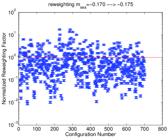
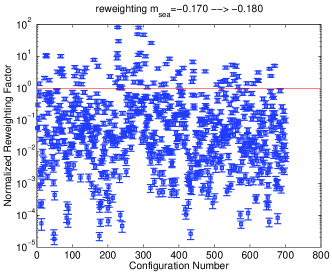
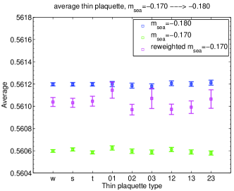
In Figure 1, we show the normalized re-weighting factors. As shown in the figure, there is a larger fraction of the configurations with small reweighting factor for the $-0.180$ case than the $-0.175$ case. Having the re-weighting factor available, we can now re-weight any physical observable of interest. As an example, we look at re-weighting the average thin plaquette. In Figure 2, we compare re-weighted various thin plaquettes to the correct values obtained from configurations generated with the correct sea quark mass. The results show that $700$ configurations provide enough statistics to re-weight from sea quark mass $-0.170$ to $-0.175$, but not to correctly reweight from $-0.170$ to $-0.180$.

Config. No.	Standard Method	Difference Method	Standard Method	Difference Method
	Double Precision	Double Precision	Mixed Precision	Mixed Precision
1	5485.76(9)	5485.78(8)	5485.91(9)	5485.77(8)
2	5484.34(9)	5484.35(8)	5484.49(9)	5484.33(8)
3	5486.57(9)	5486.63(8)	5486.73(9)	5486.62(8)

Table 1: Comparison of ${\rm{trace}}\{\log[Q_{a}(Q_{b}^{\dagger}Q_{b})^{-1}Q_{a}^{\dagger}]\}$ (standard method) and ${\rm{trace}}\{\log[Q_{a}^{\dagger}Q_{a}]\}-{\rm{trace}}\{\log[Q_{b}^{\dagger}Q_{b}]\}$ (difference method) on three configurations where $Q_{a}$ corresponds to $m_{a}=-0.170$ and $Q_{b}$ corresponds to $m_{b}=-0.180$ using $1000$ noises without dilution.

Config. Num.	Standard Method	Difference Method	Standard Method	Difference Method
	Mixed Precision	Mixed Precision	Double Precision	Double Precision
1	5+2671	105+123	6+5164	137+162
2	5+2652	103+121	6+5007	137+163
3	5+2685	106+123	6+5172	138+165

Table 2: Comparison of the number of matrix-vector products used by the standard and difference methods for a single noise vector when $S_{a}$ corresponds to $m_{0}=-0.170$ and $S_{b}$ corresponds to $m_{0}=-0.180$. For the standard method, the first number is the number of Lanczos algorithm iterations and the second number is the total number of iterations used by the CG solver during these iterations. For the difference method, the two numbers correspond to the number of iterations used by each Lanczos algorithm.

Figure 1: The normalized re-weighting factors. Left: reweighting from sea quark mass $-0.170$ to $-0.175$. Right: reweighting from sea quark mass $-0.170$ to $-0.180$.

Figure 2: Reweighted thin plaquettes compared with correct values. The horizontal axis corresponds to different types of thin plaquettes (different planes, plaquettes in the spatial directions only, etc.). Left: reweighting from sea quark mass $-0.170$ to $-0.175$. Right: reweighting from sea quark mass $-0.170$ to $-0.180$.

4 Conclusions

The application of Lanczos quadrature algorithm in mass re-weighting is studied. It is shown that it is possible to avoid the need to solve a linear system and apply the algorithm to compute each determinant separately before taking the ratio. We also showed how to get an un-biased estimator for the reweighting factors using bootstrap method. Having configurations generated with the sea quark mass we are trying to re-weight to, allowed us to compare the re-weighted observable to the correct ones and check for the range of applicability of the re-weighting procedure.

4.1 Acknowledgements

We would like to thank Stefan Meinel, Balint Joo, Robert Edwards, and Anna Hasenfratz for valuable discussions. A. Abdel-Rehim, W. Detmold and K. Orginos were supported in part by DOE grants DE-AC05-06OR23177 (JSA) and DE- FG02-04ER41302. W. Detmold was also supported by DOE OJI grant DE-SC0001784 and Jeffress Memorial Trust, grant J-968. A. Abdel-Rehim would like to thank the Cyprus Institute for support during the writing of this report.

References

- [1] A. M. Ferrenberg, and R .H .Swendsen, Phys.Rev.Lett. 61, 1988, 2635-2638.
- [2] A. Hasenfratz, R. Hoffmann, and S. Schaefer, Phys. Rev. D78, 2008, 014515, [arXiv:0805.2369]
- [3] Y. Aoki et. al., Phys.Rev. D83 (2011) 074508, [arXiv:1011.0892].
- [4] H. Ohki et. al., posPoS(LAT2009)124, [arXiv:0910.3271].
- [5] S. Aoki, et. al., Phys.Rev. D81 (2010) 074503 [arXiv:0911.2561].
- [6] Z. Bai, M. Fahey, and G. Golub, J. Comput. Appl. Math. 74 (1994)71–89.
- [7] A. Duncan, E. Eichten, and R. Sedgewick, Phys.Rev. D71 (2005) 094509 [hep-lat/0405014].
- [8] G. Bhanot and A.D. Kennedy, Phys.Lett. B157(1985)70.
- [9] R. G. Edwards and B. Joo, Nucl. Phys. Proc. Suppl. 140, 832 (2005) [arXiv:hep-lat/0409003].