Macroscopic Zeno effect and stationary flows in nonlinear waveguides with localized dissipation

Abstract

We theoretically demonstrate the possibility to observe the macroscopic Zeno effect for nonlinear waveguides with a localized dissipation. We show the existence of stable stationary flows, which are balanced by the losses in the dissipative domain. The macroscopic Zeno effect manifests itself in the non-monotonic dependence of the stationary flow on the strength of the dissipation. In particular, we highlight the importance of the parameters of the dissipation to observe the phenomenon. Our results are applicable to a large variety of systems, including condensates of atoms or quasi-particles and optical waveguides.

Since the pioneering work of Khalfin concerning the non-exponential decay of unstable atoms Khalfin the relation between the decay rate and the measurement process was in the focus of many studies. One of the fundamental results of the theory, termed after the seminal paper Zeno , as quantum Zeno effect, consists in slowing down the dynamics of a quantum system subjected to frequent measurements or to a strong coupling to another quantum system. This phenomenon was demonstrated in a rigorous mathematical framework in Zeno and received its further refinements and extension in subsequent studies theoretical . Experimentally, the quantum Zeno effect has been confirmed for single ions Itano , ultracold atoms in accelerated optical lattices Zeno_accel_lattice , atomic spin motion controlled by circularly polarized light Zeno_spin , an externally driven mixture of two hyperfine states of neutral atoms Zeno_mixture , photons in a cavity Bernu2008 and the production of cold molecular gases in an optical lattice Zeno_molecule . It has also been predicted Zoller ; KS that the tunneling dynamics of particles in a double-well potential can be slowed down if the particles are removed from one of the wells. Qualitatively similar results for the suppression of atom losses in an open Bose-Hubbard chain were reported in BoseHubbard . In the limit of an infinitely strong measurement of particles in a given spatial domain it has been shown that the system is projected onto a unitary dynamics in the loss-free domain Facchi2008 .

The Zeno effect is sometimes also understood in more general terms as the effects of changing a decay law depending on the frequency of measurements Zeno_Gen . Applying this definition to a macroscopic quantum system, like a gas of condensed bosonic atoms and, taking into account that in the macroscopic dynamics the frequency of measurement can be interpreted as the strength of the induced dissipation KS , the effect of the measurement on the decay of the quantum system can be viewed as the effect of dissipation on the macroscopic characteristics of the system. Here we assume this interpretation of the phenomenon and address the questions how the appearance of localized losses in a waveguide is connected to the appearance of Zeno-like dynamics. In order to emphasize the distinction of the latter statement of the problem with respect to already standard and widely accepted notion of quantum Zeno effect, below we refer to macroscopic Zeno effect (MZE) bearing in mind its meanfield manifestation.

Losses are ubiquitous for real quantum systems due to the coupling to an environment. Very often, the loss processes are also spatially localized. They can be either externally engineered, e.g. with the tip of a scanning probe microscope, a local probe in a quantum gas, an absorbing spatial domain, or they can be intrinsically present in the form of defects and impurities. One can therefore expect, that the MZE can manifest itself in a wide class of physical systems, including exciton-polaritons excitonpolaritons , magnon gases magnons , surface plasmons surfaceplasmons , and optics of nonlinear Kerr media AKS .

We study one-dimensional nonlinear waveguides governed by the nonlinear Schrödinger equation

$$i\Psi_{t}=-\Psi_{xx}+g|\Psi|^{2}\Psi-i\gamma(x)\Psi,$$ (1)

where $g$ the nonlinearity parameter and the local loss processes are modelled by $i\gamma(x)$ (for a review on the application of complex potentials see e.g. Muga ). Since the localized dissipation is applied to a homogeneous condensate, i.e. it breaks the translational invariance of the system, it can be referred to as a dissipative defect BKPO . We are interested in stationary flows, which correspond to a situation when an incoming flux of a particles from both ends of the waveguide is exactly balanced by the losses in the dissipative domain. Notice that in such a statement counting of lost particles is replaced by computing the number of particles that must be loaded into the system in order to compensate the losses.

In Fig. 1 we show several examples of how such a scenario can be realized experimentally in different physical systems. While our approach is applicable to a large variety of physical situations, the systems we have in mind are those described in GUHO ; Ott ; BKPO ; Guarrera2011 , i.e. an atomic BEC subjected to removal of atoms. In this last case, the time and the coordinate are respectively measured in units of $(2\omega_{\bot})^{-1}$ and $a_{\bot}/2$, where $a_{\bot}$ and $\omega_{\bot}$ are the transverse linear oscillator length and the frequency of the transverse trap, while $g=a_{s}n_{0}$, being $a_{s}$ the scattering length and $n_{0}$ the unperturbed linear density of the condensate. In the following we consider only the case $g>0$ which describes repulsive inter-atomic interactions (or defocusing Kerr media in optical applications).

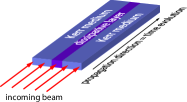
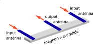
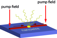
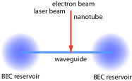
Figure 1: Possible experimental scenarios to observe the MZE: nonlinear optical waveguide (upper left), a magnon waveguide (upper right), a plasmonic nanostructure (lower left), an atomic BEC in a waveguide and two reservoirs (lower right).

The dissipation is described by the nonnegative localized function $\gamma(x)$, which is characterized by two control parameters: its amplitude $\Gamma_{0}$ and characteristic width $\ell$. It is convenient to set $\gamma(x)=\Gamma_{0}f(x/\ell)$ where $f(x)$ is a known smooth function such that $\max_{x}|f(x)|=f(0)\sim 1$ and $\max_{x}|f_{x}(x)|\sim 1$. Then $\Gamma_{0}$ and $\ell$ are proportional to the intensity of the defect: $\int_{-\infty}^{\infty}\gamma(x)dx\propto\Gamma_{0}\ell$. We will also assume the most typical experimental situation where $\gamma(x)$ is an even function: $\gamma(x)=\gamma(-x)$ with only one maximum at $x=0$. Having in mind the experiments of Ref. GUHO ; Ott ; Guarrera2011 one can estimate that $\Gamma_{0}\sim I\sigma_{ion}/(e_{0}\omega_{\bot})$ where $I$ is the current of the electron beam, $e_{0}$ is the electric charge of the electron, and $\sigma_{ion}$ is the total ionization cross section.

The stationary flows are sought in the form $\Psi_{st}(t,x)=\rho(x)\exp\left[i\int_{0}^{x}v(s)ds-i\mu t\right]$, where $v(x)$ is the superfluid velocity, $\mu$ is the chemical potential, and $\rho^{2}(x)=n(x)$ is the density. Substituting $\Psi_{st}(t,x)$ into Eq. (1) we obtain

$$\rho_{xx}+\mu\rho-g\rho^{3}-j^{2}\rho^{-3}=0,\quad j_{x}+\gamma(x)\rho^{2}=0$$ (2)

with $j(x)=v(x)n(x)$ being the superfluid current. We are interested in solutions of Eqs. (2) with a constant density at infinity: $\lim_{|x|\to\infty}|\rho(x)|=\rho_{\infty}$. Then $\mu=j_{\infty}^{2}\rho_{\infty}^{-4}+g\rho_{\infty}^{2}$, where $j_{\infty}=\mp\lim_{x\to\pm\infty}j(x)$ is a positive constant. For any stationary flow, the loss of particles in the defect has to be balanced by the incoming current $j_{\infty}$. The main objective of the present study is to show the existence of such stationary flows and to explore the dependence of the current $j_{\infty}$ on the parameters of the defect.

First, we consider an example that allows for an exact solution, extending the result of BKPO . We assume a dissipative defect of the particular form $\displaystyle{\gamma(x)={3\Gamma_{0}}{\mathrm{sech}^{2}(x/\ell)}}$. Then it is a straightforward to show that $\rho(x)=\tanh(x/\ell)$ and $j(x)=-\Gamma_{0}\ell\tanh^{3}(x/\ell)$ are solutions of the system (2) provided that $\ell^{2}(g+\Gamma_{0}^{2}\ell^{2})=2$. Thus the incoming flux is linearly proportional to the intensity of the dissipative defect: $j_{\infty}=\Gamma_{0}\ell$, and in order to obtain a stationary solution, increase of the strength of the dissipation must be compensated with an increase of the incoming flux. In other words, if the incoming flux of particles is increased, the excess particles can only be removed by a stronger defect. While this result is quite intuitive, we show below that it does not hold in general. In particular, we will show that for appropriate parameters, an increasing flux can be compensated by a weaker defect.

We now focus on a dissipation with finite support: $\gamma(x)\equiv 0$ if $|x|>\ell$. This form of the dissipative term models, in particular, the electronic beam used in GUHO ; Ott . In order to decrease numerical errors we choose $\gamma(x)$ to be smooth at the edges of the dissipative domain: $\gamma(x)=\Gamma_{0}\left(1-x^{2}/\ell^{2}\right)^{2}$ if $|x|<\ell$.

Since Eq. (2) is not integrable – unlike its conservative counterpart where $\gamma(x)\equiv 0$ – it is convenient to treat $\Gamma_{0}$ as a parameter that increases departing from zero. Experimentally, this would correspond to an adiabatic increase of the defect intensity. For $\Gamma_{0}=0$ one recovers two well-known solutions: a constant density $\rho(x)=\rho_{\infty}$ and a dark soliton $\rho(x)=\rho_{\infty}\tanh(\sqrt{g/2}\,\rho_{\infty}x)$ [$j(x)\equiv 0$ for both solutions]. When the defect is adiabatically switched on, the constant density and the dark soliton give origin to two branches of solutions. The branch bifurcating from the constant density consists of symmetric flows, for which the relation $\rho(x)=\rho(-x)$ holds. The flows that branch off from the dark soliton are antisymmetric, $\rho(x)=-\rho(-x)$. From the second of Eqs. (2) it follows that both the symmetric and antisymmetric flows possess odd currents: $j(x)=-j(-x)$.

Considering behavior of the solutions in the vicinity of $x=0$, for the symmetric flows we obtain $\rho_{xx}(0)=\rho(0)[g(\rho^{2}(0)-\rho_{\infty}^{2})-j_{\infty}^{2}\rho_{\infty}^{-4}]$. Thus, employing a physically obvious condition $\rho_{\infty}>\rho(0)>0$, we find $\rho_{xx}(0)<0$. We therefore arrive at the counterintuitive conclusion that for the symmetric flows the atomic density $n(x)$ has a local maximum in the point of maximal dissipation.

On the other hand, for $x\to\infty$ both symmetric and antisymmetric flows behave as

$$\rho_{\infty}-\rho(x)\propto e^{-\sqrt{\Lambda}x},\mbox{ where }\Lambda=2g\rho_{\infty}^{2}-{4j_{\infty}^{2}}{\rho_{\infty}^{-4}}.$$ (3)

Thus, for a given density $\rho_{\infty}$ there exists an upper bound for the maximal current $j^{max}_{\infty}=\sqrt{g}\rho_{\infty}^{3}/\sqrt{2}$ above which no stationary flow can exist.

In Fig. 2 (a) [Fig. 2 (b)] we show the density profiles $n(x)$ of symmetric [antisymmetric] flows for different values of the dissipation strength $\Gamma_{0}$. We observe that for the symmetric flows, the density possesses two deep local minima. For a weak dissipation (e.g. $\Gamma_{0}=0.01$) the minima are situated outside the dissipative domain, which allows to compute the exact value of the density in these minima: $n_{min}={2j_{\infty}^{2}}{\rho_{\infty}^{-4}}/g$. As the strength of the dissipation grows, the minima move from $\pm\infty$ towards the center and eventually enter the dissipative domain. For antisymmetric flows the dependence of the density on $\Gamma_{0}$ is much weaker pronounced [the curves for different $\Gamma_{0}$ are hardly distinguishable on the scale of the Fig. 2 (b)].

Now our goal is to study the dependence $j_{\infty}$ vs $\Gamma_{0}$. The typical results for the symmetric [antisymmetric] flows are illustrated in Fig. 2 (c) [Fig. 2 (d)] . When the nonlinearity is strong enough ($g=1$), for both types of the flows one can clearly see a global maximum of $j_{\infty}(\Gamma_{0})$. When $\Gamma_{0}$ exceeds the value corresponding to this maximum, the required current $j_{\infty}$ decreases. This is the manifestation of the MZE.

In order to observe the MZE in an experiment, it is important that the solutions are stable. To explore the stability of the flows, we substitute $\Psi(t,x)=\Psi_{st}(t,x)+e^{-i\mu t}\left[a_{+}(x)e^{\lambda t}+a_{-}^{*}(x)e^{\lambda^{*}t}\right]$ into Eq. (1), linearize it with respect to $a_{\pm}(x)$, and solve the obtained linear eigenvalue problem. Instability occurs if there exists an eigenvalue $\lambda$ with positive real part $\lambda_{r}$. The results of the analysis are shown in Fig. 2 (c)–(e). For the symmetric flows presented in Fig. 2 (c), small values of $\Gamma_{0}$ do not allow for stable stationary flows (see the dotted fragments of the lines). For instance, the symmetric flow with two local minima situated outside of the dissipative domain [shown in Fig. 2 (a) and corresponding to $\Gamma_{0}=0.01$] is unstable. For larger values of $\Gamma_{0}$ the symmetric flows become stable. We have observed that the two minima of a stable symmetric flow are always located in the dissipative domain. All antisymmetric flows shown in Fig. 2 (d) are stable. Most importantly, the parameter range, in which the MZE is observed, has only stable flows. From experimental point of view, the existence of stable symmetric flows is very appealing, as symmetric flows arise from the overall (symmetric) ground state of the system.

We now elaborate on the role of the size of the defect. In Fig. 2 (e), we show the currents vs $\ell$ for a fixed $\Gamma_{0}$. As the defect becomes wider, one might expect a monotonic increase of $j_{\infty}$. As can be seen from the graph, this behavior is indeed encountered, however only in average. Locally it is superimposed by a resonance-like structure which tends to enhance the current for certain defect sizes. We also find that stable solutions only appear when the $j_{\infty}(\ell)$ is a growing function and that (up to a certain degree of accuracy) the domains of stability of the symmetric flows coincide with the domains of instability of the antisymmetric flows and vice versa.

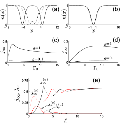
Figure 2: (a): Density distributions $n(x)$ for symmetric flows for $g=1$ and $\ell=4$ and different values of $\Gamma_{0}$. Solid line: $\Gamma_{0}=0.01$, dashed line: $\Gamma_{0}=1$, dotted line: $\Gamma_{0}=10$. (b): Density distributions $n(x)$ for antisymmetric flows for $g=1$ and $\ell=1$. Solid line: $\Gamma_{0}=0.1$, dashed line: $\Gamma_{0}=1$, dotted line: $\Gamma_{0}=10$. (c) and (d): Current vs strength of the dissipation for symmetric flows (with $\ell=4$) and for antisymmetric flows (with $\ell=1$) obtained for $g=0.1$ and $g=1$; stable (unstable) flows correspond to the solid (dotted) fragments of the curves; (e): Currents and instability increments vs width of the defect for symmetric [${(s)}$] and antisymmetric [${(a)}$] flows for $g=1$ and $\Gamma_{0}=1$. In all panels $\rho_{\infty}=1$.

So far, we have encountered two different situations: in the case of the $\mathrm{sech}^{2}$-shaped dissipation, the branch of stationary flows does not show the MZE. In the case of the dissipation with finite support, the MZE has various manifestations. The difference can be explained by looking at the asymptotic behavior of the corresponding flows. In the case of the $\mathrm{sech}^{2}$-shaped dissipation, the asymptotical behavior at $x\to\infty$ of the density is completely determined by the characteristic width $\ell$ of the defect: $\rho_{\infty}-\rho(x)\sim 2e^{-2x/\ell}$, while the flows supported by the dissipation with finite support behave according to Eqs. (3). Moreover, Eqs. (3) imply that there exists the maximal possible current $j^{max}_{\infty}$. It appears that the presence of such a threshold is a signature of the MZE. No such threshold exists for the stationary flows with the $\mathrm{sech}^{2}$-shaped dissipation: the current $j_{\infty}$ can be arbitrarily large and the MZE is not found.

However, the $\mathrm{sech}^{2}$-shaped dissipation still does not forbid the MZE in principle, since flows obeying Eqs. (3) can also be found in this case. Let us revisit the dissipation of the form $\gamma(x)=3\Gamma_{0}\mathrm{sech}^{2}(x/\ell)$. Substituting $\rho(x)=\rho_{\infty}-\rho_{1}(x)$, where $\rho_{1}(x)=o(1)$ as ${x\to\infty}$, into Eqs. (2) and neglecting the terms of smaller order, one observes that for $x\gg 1$ the function $\rho_{1}(x)$ is described by the equation $\rho_{1,xx}-\Lambda\rho_{1}=12{j_{\infty}\Gamma_{0}\ell}{\rho_{\infty}^{-1}}e^{-2x/\ell}$. For $\rho_{1}(x)$ to obey the asymptotics (3) the two conditions must be fulfilled: (i) $\Lambda>0$ – gives the maximal current: $j_{\infty}<j^{max}_{\infty}$; (ii) $\sqrt{\Lambda}<2/\ell$ – yields the minimal possible current: $j_{\infty}>j^{min}_{\infty}=\rho_{\infty}\sqrt{g\rho_{\infty}^{4}/2-\ell^{-2}}$ (if the expression under the radical is negative, then $j^{min}_{\infty}=0$). As $\ell$ grows, $j^{min}_{\infty}$ approaches $j^{max}_{\infty}$. Hence, the range of currents allowing for the solutions which obey Eqs. (3) decreases. This leads us to the conjecture that rapidly decaying dissipation is favorable for the observation of the macroscopic Zeno effect. In particular, the defects decaying faster than exponentially are more likely to display the MZE than ones obeying exponential decaying.

We close this Letter with a discussion of possible experimental observation of the found MZE. The incoming flux of particles has to be generated at both ends of the waveguide. This can be achieved by controlled pumping terms in the case of quasiparticles or by reservoirs in the case of real particles. For light propagating in a non-linear waveguide, such boundary conditions appear rather naturally. But even for a finite system with no reservoir, one can speculate that a quasi stationary state is established on intermediate time scales in a transient regime: if the defect is switched on in a finite system that is initially in its ground state, the stationary flow will develop out of symmetric initial conditions and will retain its symmetry with increasing dissipation. With time, a flow of particles towards the defect is created which can mimic the boundary conditions, applied in the preceding discussion. The condition of having a defect that drops faster than exponentially can be easily realized in most of the experimental implementations suggested above.

We now support this reasoning by illustrating the generation of stationary flows through direct integration of Eq. (1) on a finite domain subject to the boundary conditions $\Psi(t,\pm L)=\rho_{\infty}e^{-i\mu t}$ (here $L$ is the half-width of the computational domain). In Fig. 3 we show the temporal evolution of the atomic density for three different widths of the defect. For all the shown evolutions, the initial density is taken to be constant and the chosen boundary conditions fix the density and the chemical potential at the edges of the computational domain. Figure 3 (a) shows the evolution for a set of parameters, where a stable symmetric stationary flow exists. After initial decrease of the density at the location of the defect, the system achieves the stationary flow. In the vicinity of the origin one clearly observes the two local minima residing inside the defect. Indeed, the density approaches eventually the stationary flow profile not only in the vicinity of the origin but in the entire computational domain. However, if the symmetric flow is not expected to be stable [Fig. 3 (b) and Fig. 3 (c)], then the density profile shows ongoing distortions in the vicinity of the origin and eventually loses the symmetry. For the cases shown in panels (b) and (c), the density tends to approach a profile corresponding to a stable antisymmetric flow which exists for the chosen values of $\ell$ and $\Gamma_{0}$ [recall that the domains of the stability of the symmetric and antisymmetric flows alternate as shown in Fig. 2 (e)]. However, in the cases (b) and (c) truly stationary antisymmetric flows are not established because the chosen boundary conditions can support only symmetric flows, which are unstable for the chosen parameters.

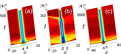
Figure 3: Evolution of the density $|\Psi(t,x)|^{2}$ starting from the initial data $\Psi(0,x)=1$. For all the shown panels $\rho_{\infty}=g=\Gamma_{0}=1$. (a): The width of the defect is $\ell=4$. The generation of the symmetric stationary flow occurs. (b) and (c): The width of the defect is $\ell=2$ and $\ell=6$ respectively. The symmetric flows are unstable, and therefore no stationary flow is established.

In summary, we have analyzed a non-linear waveguide with a localized dissipative defect. We found evidence for the appearance of the macroscopic Zeno effect for specific boundary conditions and have analyzed to role of the interaction and the defect size. The observed macroscopic Zeno effect is intrinsically related to the existence of the stable stationary flows and is expressed through nonmonotonic dependence of the intensity of the dissipation on the density of incoming currents. The proofed existence of stable solutions for symmetric flows is very important, as these solutions correspond to many natural experimental situations.

- (1) L. A. Khalfin, Dokl. Akad. Nauk SSSR 115, 277 (1957) [Sov. Phys. Dokl. 2, 232 (1958)]; Zh. Eksp. Teor. Fiz. 33, 1371 (1958) [Sov. Phys. JETP-USSR 6, 1053 (1958)].
- (2) B. Misra and E. C. G. Sudarshan, J. Math. Phys. Sci. 18, 756 (1977).
- (3) A. G. Kofman and G. Kurizki, Nature (London) 405, 546 (2000); Phys. Rev. Lett. 87, 270405 (2001); P. Facchi and S. Pascazio, ibid. 89, 080401 (2002); A. Barone, G. Kurizki, and A. G. Kofman, ibid. 92, 200403 (2004); I. E. Mazets, G. Kurizki, N. Katz, and N. Davidson, ibid. 94, 190403 (2005).
- (4) W. M. Itano, D. J. Heinzen, J. J. Bollinger, and D. J. Wineland, Phys. Rev. A 41, 2295 (1990).
- (5) M. C. Fischer, B. Gutiérrez-Medina, and M. G. Raizen, Phys. Rev. Lett. 87, 040402 (2001).
- (6) T. Nakanishi, K. Yamane, and M. Kitano, Phys. Rev. A 65, 013404 (2001).
- (7) E. W. Streed, J. Mun, M. Boyd, G. K. Campbell, P. Medley, W. Ketterle, and D. E. Pritchard, Phys. Rev. Lett. 97, 260402 (2006).
- (8) J. Bernu et al., Phys. Rev. Lett. 101, 180402 (2008).
- (9) N. Syassen et al., Science 320, 1329 (2008).
- (10) J. I. Cirac, A. Schenzle, and P. Zoller, Europhys. Lett. 27, 123 (1994).
- (11) V. S. Shchesnovich and V. V. Konotop, Phys. Rev. A 81, 053611 (2010).
- (12) D. Witthaut, et. al. Phys. Rev. A 83, 063608 (2011); P. Barmettler, C. Kollath, Phys. Rev. A 84 041606 (2011).
- (13) P. Facchi and S. Pascazio J. Phys. A: Math. Theor. 41, 493001 (2008).
- (14) L. A. Khalfin, Usp. Fiz. Nauk 160, 185 (1990) [Sov. Phys. Usp. 33 868, (1990)].
- (15) A. Amo, et. al. Nature, 457, 291 (2009); A. Amo, et. al. Nature Photonics, 4, 361 (2010).
- (16) S. O. Demokritov, et al. Nature 443, 430 (2006); S. Schäfer, V. Kegel, A. A. Serga, B. Hillebrands, and M. P. Kostylev, Phys. Rev. B 83, 184407 (2011).
- (17) M. Aeschlimann, et al. Science 333, 1723 (2011); Z. Ma, et al. Appl. Phys. Lett. 96, 051119 (2010).
- (18) F. Kh. Abdullaev, V. V. Konotop, and V. S. Shchesnovich, Phys. Rev. A 83, 043811 (2011); F. Kh. Abdullaev, V. V. Konotop, M. Ögren, and M. P. Sørensen, Opt. Lett. 36, 4566 (2011).
- (19) J. G. Muga, J. P. Palao, B. Navarro, and I. L. Egusquiza, Phys. Rep. 395, 357 (2004).
- (20) V. A. Brazhnyi, V. V. Konotop, V. M. Pérez-García, and H. Ott, Phys. Rev. Lett. 102, 144101 (2009).
- (21) T. Gericke, C. Utfeld, N. Hommerstad, and H. Ott, Las. Phys. Lett. 3, 415 (2006).
- (22) T. Gericke, P. Würtz, D. Reitz, T. Langen, and H. Ott, Nature Phys. 4, 949 (2008).
- (23) V. Guarrera et al., Phys. Rev. Lett. 107, 160403 (2011).